Heterogeneous Spillover Networks and Spatial–Temporal Dynamics of Systemic Risk Transmission: Evidence from G20 Financial Risk Stress Index

Abstract

With the continuous integration of globalization and financial markets, the linkage of global financial risks has increased significantly. This study examines the risk spillover effects and transmission dynamics among the financial markets in G20 countries, which together represent over 80% of global GDP. With increasing globalization and the interconnectedness of financial markets, understanding risk transmission mechanisms has become critical for effective risk management. Previous research has primarily focused on price volatility to measure financial risks, often overlooking other critical dimensions such as liquidity, credit, and operational risks. This paper addresses this gap by utilizing the vector autoregressive (VAR) model to explore the spillover effects and the temporal and spatial characteristics of risk transmission. Specifically, we employ global and local Moran indices to analyze spatial dependencies across markets. Our findings reveal that the risk linkages among the G20 financial markets exhibit significant time-varying characteristics, with spatial risk distribution showing weaker dispersion. By constructing a comprehensive financial risk index system and applying a network-based spillover analysis, this study enhances the measurement of financial market risk and uncovers the complex transmission pathways between sub-markets and countries. These results not only deepen our understanding of global financial market dynamics but also provide valuable insights for the design of effective cross-border financial regulatory policies. The study’s contributions lie in enriching the empirical literature on multi-dimensional financial risks, advancing policy formulation by identifying key risk transmission channels, and supporting international risk management strategies through the detection and mitigation of potential contagion effects.

1. Introduction

In recent years, global events such as economic crises, geopolitics, trade frictions, and major sudden public health security occur frequently, and the risk management of financial markets has become an important topic in global economic research. The global financial crisis in 2008 and the COVID-19 outbreak in 2020 further exposed the complexity of risk transmission between financial markets and the huge impact of emergencies on the global economy [1,2]. These events have underscored the critical need to understand and manage systemic risk transmission in financial markets, especially as globalization and economic interdependence continue to increase [3,4].

The spillover effect of financial market volatility means that the volatility of a country or region in a financial market will be transmitted to other countries or regions through various channels, leading to the synchronous increase or weakening of market volatility on a global scale. The transmission of financial risks stems from the high dependence and complex correlation between financial markets. Existing research shows that the financial market risks between different countries do not exist in isolation, but pass on and influence each other through various channels [5,6]. The high volatility of financial markets will not only affect the economic stability of China, but also have a significant impact on other countries (regions) through trade, investment, exchange rates, and other channels [7,8,9]. However, while much research has focused on risk spillover effects, significant gaps remain in our understanding of the dynamic and heterogeneous nature of these spillovers, particularly in relation to multiple markets over various timeframes. Specifically, the research problem this paper addresses is the lack of comprehensive and systematic analysis of the overall risk, sub-market risks, and the cross-market risk correlation network and transmission pathways, particularly in the context of the G20 financial markets.

At the same time, studying the space–temporal characteristics of financial markets is also an important dimension to explore to reveal the risk transmission path. Research shows that risk transmission in financial markets is dynamic and heterogeneous in time and space [10,11]. There are significant differences in the risk transmission path and intensity between markets in different time windows [12]. In the spatial dimension, the closeness of geographical proximity also has a certain influence on risk transmission between markets [13].

As major global economies, the G20 countries have closely observed the risk transmission relationships between their financial markets. The G20 countries account for more than 80% of global GDP and are at the core of the global financial system. Their financial markets are highly interconnected and significantly influence global financial stability. Thus, understanding the risk spillover effects and transmission mechanisms within the G20 is essential for developing effective international financial regulatory policies and enhancing global financial stability. Governments in various G20 nations have introduced a series of measures aimed at strengthening financial supervision, improving market transparency, and boosting the financial system’s resilience to risks [14,15,16]. These include enhancing the risk management capabilities of financial institutions, improving market risk monitoring frameworks, and promoting international financial regulatory cooperation to address cross-border risks [13].

This study aims to address the gap in the literature by offering a comprehensive analysis of the risk spillover effects and transmission dynamics across the G20 financial markets. By rigorously examining these interlinkages, this study clarifies the mechanisms through which financial risks propagate across borders and market segments, providing a robust empirical foundation for evidence-based policy formulation. The key contribution of this research is the innovative integration of a risk spillover matrix with network analysis methodologies to quantitatively assess both the structure and evolution of systemic risk, enhancing the understanding of cross-market contagion. This approach advances theoretical understanding and provides actionable insights for enhancing global financial regulatory coordination and resilience.

2. Literature Review

In recent years, the study of risk transmission in global financial markets has gained significant attention. Diebold and Yilmaz (2009) pioneered the development of a risk spillover index based on the variance decomposition of prediction error [17]. This index quantifies the risk spillover effect between different markets and reveals the complex risk transmission pathways among global financial markets. Their groundbreaking work laid the foundation for a growing body of research on spillovers between financial markets, particularly focusing on volatility transmission and the methodologies used to capture these dynamics.

Subsequently, numerous studies have utilized the vector autoregression (VAR) model to analyze the spillover effects of fluctuations across financial markets. For instance, Lanne and Saikkonen (2011) employed a non-causal VAR model to study volatility spillover effects in the stock market, highlighting the non-causal nature of variable relationships [18]. Caporin et al. (2018) used the VAR model to analyze the spillover effects of exchange rate fluctuations in global financial markets [19,20]. Their research explored volatility transmission and risk spillovers within the exchange rate market, uncovering the intercorrelations and dynamic characteristics of exchange rate movements. While these studies contribute to our understanding of how shocks propagate across markets, their scope is often limited to a single asset class or market, which constrains the broader applicability of their findings. Unlike previous studies that focus on specific asset classes or markets, this paper introduces a comprehensive approach that integrates multiple financial markets, including equity, foreign exchange, and bond markets, into a unified risk spillover framework. Additionally, Lau and Go (2018) [21], Maitra and Dawar (2019) [22], and Zhao et al. (2020) [23] have also adopted this approach in their studies. Although these studies expanded the application of VAR to different asset classes and time periods, there remains a gap in integrating diverse financial markets into a cohesive risk spillover framework.

Several researchers have focused on the spillover effects of volatility among financial markets from the perspective of yield and volatility (Xiao and Li, 2014; Li et al., 2019; Yu, et al., 2019; Zhou, et al., 2021) [24,25,26,27]. Research findings regarding the direction of volatility spillovers have been mixed. Chen et al. (2009) and He et al. (2013) identified two-way asymmetric fluctuation spillover effects between financial markets [28,29], while Chen et al. (2009) also proposed that certain financial markets exhibit only one-way volatility spillovers [30]. These mixed results underscore the complexity of spillover dynamics and highlight the need for more nuanced methodologies to capture such complexities across multiple markets.

In terms of research on the spatial and temporal characteristics of risk transmission, Zhao (2020) [23] constructed a foreign exchange market pressure risk overflow network for over 30 countries. By analyzing the time-varying characteristics and spatial evolution of the global foreign exchange market pressure risk overflows from 1997 to 2019, significant risk spillover effects within the foreign exchange market were identified. This research emphasizes the need to consider both spatial and temporal dimensions to understand risk transmission, an aspect that remains underexplored in many studies.

However, the existing literature has certain limitations. First, most studies focus on price volatility as the primary measure of financial risk, neglecting other crucial risk factors such as liquidity risk, credit risk, and operational risk. For instance, during the 2008 global financial crisis, the liquidity crunch in financial markets had a significant impact on overall stability; yet, the research relying solely on price volatility did not fully capture this dimension. Second, much of the research is limited to analyzing the spillover effects between just one or two financial markets. This narrow focus prevents a comprehensive understanding of risk dynamics across the entire global financial system. Furthermore, there is a gap in the literature concerning the interaction between various sub-markets and their collective impact on financial stability. Finally, while some studies have explored the risk transmission paths within financial markets, they often overlook the underlying factors that influence these relationships, such as macroeconomic policies, geopolitical events, and technological changes in financial trading systems. Additionally, the spatial and temporal evolution of these relationships is often insufficiently studied.

In contrast to these studies, we measure the overall and sub-market risk indices, employing risk spillover matrices and network analysis methods to explore the risk transmission relationships among G20 countries. This approach facilitates a more comprehensive understanding of global risk spillovers across multiple dimensions. Furthermore, it investigates the underlying factors driving these risk transmission relationships, along with the spatial and temporal characteristics of financial market correlations. The primary contributions of this paper are as follows: (1) it provides an improved measurement of financial market risk by using the financial market risk index; (2) it systematically examines the overall risk, sub-market risk and cross-market risk correlation network and transmission pathways of financial markets, and contributes incrementally to the research on risk spillover effects; and (3) by examining the spatial and temporal characteristics of financial market correlations, this study uncovers the complex structure and evolutionary trends of the global financial market, which not only provides a new perspective for understanding the dynamic characteristics of the global financial market, but also serves as a significant reference for policymakers when dynamically adjusting their policies.

3. Research Methods and Model Construction

3.1. Measurement of Risk Method in Global Financial Markets

The financial risk pressure index is calculated and synthesized by real-time high-frequency data indicators that reflect the fluctuations of a financial market. It can not only quantify the risk assessment of the financial system of a country or a region, but also continuously reflect the pressure faced by the financial system of a country or region. This paper refers to the pressure index model of Sachs, et al. (1996) [31] and the early warning study on financial market risk of Wang and Hu (2014) [32]. Unlike Sachs et al. (1996) [31], our methodology incorporates additional sub-market indices and redefines the weighting system. Specifically, we include a money market risk pressure index based on the volatility of interest rate market returns, a foreign exchange market pressure index influenced by the fluctuations in foreign exchange reserves, and a stock market risk pressure index that accounts for both the levels and volatility of monthly stock market index yields. Furthermore, we redefine the weights by considering the volatility of each individual market’s financial conditions, employing the reciprocal of the standard deviation for each sub-market as the basis for these weights. These enhancements allow for a more comprehensive and nuanced assessment of financial risk pressures across various market segments. The calculation formula for the financial market risk pressure index is as follows:

$$\mathrm{F}\mathrm{R}\mathrm{I}={\mathsf{\omega }}_{\mathrm{c}}\mathrm{C}\mathrm{R}\mathrm{I}+{\mathsf{\omega }}_{\mathrm{e}}\mathrm{E}\mathrm{R}\mathrm{I}+{\mathsf{\omega }}_{\mathrm{s}}\mathrm{S}\mathrm{R}\mathrm{I}$$

(1)

$${\mathsf{\omega }}_{\mathrm{m}}={\displaystyle \frac{1}{{\mathsf{\sigma }}_{\mathrm{m}}}}/({\displaystyle \frac{1}{{\mathsf{\sigma }}_{\mathrm{c}}}}+{\displaystyle \frac{1}{{\mathsf{\sigma }}_{\mathrm{e}}}}+{\displaystyle \frac{1}{{\mathsf{\sigma }}_{\mathrm{s}}}}),\mathrm{m}=\mathrm{c},\mathrm{e},\mathrm{s}$$

(2)

Equation (1) shows the financial market risk pressure index FRI; CRI, ERI, and SRI on the right are the money market risk pressure index, the foreign exchange market risk pressure index, and the stock market pressure index, respectively. According to the IMF report (2009), the reciprocal of the standard deviation of each sub-market is taken as the weight ${\mathsf{\omega }}_{\mathrm{m}}$ [33]. Equation (2) constructs the weight equation, where σ represents the standard deviation. The greater the value of the FRI index, the greater the risk of the country’s financial markets.

The reciprocal proportion of the standard deviation as the weight is mainly due to the following two considerations. The first is reliability, which balances the volatility of each indicator. The financial stress index consists of several indicators reflecting the risk of different markets, and their volatility is different. For example, stock markets can fluctuate sharply in the short term, while money markets are relatively stable. By using the inverse of the standard deviation as the weight, the volatility of each index can be balanced so that an index with large volatility has less influence in the composite index, thus making the financial pressure index more stable and representative. The larger the standard deviation in the secondary market, the more unstable it is. A small weight can avoid excessive interference from the fluctuating secondary market with an overall risk assessment, thus ensuring the reliability of the overall index and making it more representative of the risk situation of the whole financial market. The second is comprehensiveness, which reflects the importance of each indicator. The financial market consists of several sub-markets, each of which has its own characteristics and risk volatility degree, which can be reflected by the reciprocal of the standard deviation. Less volatile indicators are often more reflective of long-term trends and systemic risks, so giving them more weight can better capture the overall pressures of the financial system. When balancing the influence of different sub-markets in a comprehensive calculation, the comprehensive index can reflect the overall financial risk level more comprehensively and objectively.

In this paper, the volatility of interest rate market returns is used to measure the risk for the whole money market, shown in Equation (3); the risk pressure index of the foreign exchange market is constructed by the change of foreign exchange reserves, shown in Equation (4), and the specific model of the stock market risk pressure index is shown in Equation (5). In these equations, i and t represent the country and month, respectively, ${∆\mathrm{R}}_{\mathrm{i}\mathrm{t}}$ represents the first order difference of the interest rate, $∆\mathrm{E}$ and $∆\mathrm{R}\mathrm{E}\mathrm{E}\mathrm{R}$ respectively represent the first order difference of the exchange rate and the foreign exchange reserves, SR represents the change level of the monthly stock market index yield, SV indicates the volatility of the stock market yield reflects the uncertainty and risk pressure of the stock market; and are the mean and standard deviation, respectively.

$${\mathrm{C}\mathrm{R}\mathrm{I}}_{\mathrm{i}\mathrm{t}}={\displaystyle \frac{{∆\mathrm{R}}_{\mathrm{i}\mathrm{t}}-{\mathsf{\mu }}_{{∆\mathrm{R}}_{\mathrm{i}}}}{{\mathsf{\sigma }}_{{∆\mathrm{R}}_{\mathrm{i}}}}}$$

(3)

$${\mathrm{E}\mathrm{R}\mathrm{I}}_{\mathrm{i}\mathrm{t}}={\displaystyle \frac{{∆\mathrm{E}}_{\mathrm{i}\mathrm{t}}-{\mathsf{\mu }}_{{∆\mathrm{E}}_{\mathrm{i}}}}{{\mathsf{\sigma }}_{{∆\mathrm{E}}_{\mathrm{i}}}}}-{\displaystyle \frac{{∆\mathrm{R}\mathrm{E}\mathrm{E}\mathrm{R}}_{\mathrm{i}\mathrm{t}}-{\mathsf{\mu }}_{{∆\mathrm{R}\mathrm{E}\mathrm{E}\mathrm{R}}_{\mathrm{i}}}}{{\mathsf{\sigma }}_{{∆\mathrm{R}\mathrm{E}\mathrm{E}\mathrm{R}}_{\mathrm{i}}}}}$$

(4)

$${\mathrm{S}\mathrm{R}\mathrm{I}}_{\mathrm{i}\mathrm{t}}={\mathrm{S}\mathrm{V}}_{\mathrm{i}\mathrm{t}}-{\mathrm{S}\mathrm{R}}_{\mathrm{i}\mathrm{t}}, {\mathrm{S}\mathrm{R}}_{\mathrm{i}\mathrm{t}}=\ln ({\mathrm{S}}_{\mathrm{i}\mathrm{t}}-{\mathrm{S}}_{\mathrm{i},\mathrm{t}-1}), {\mathrm{S}\mathrm{V}}_{\mathrm{i}}=\sqrt{{\sum }_{\mathrm{t}=1}^{\mathrm{T}}{\mathrm{S}\mathrm{R}}_{\mathrm{i}\mathrm{t}}^2}$$

(5)

3.2. Analysis Model of Risk Transmission in Global Financial Markets

Currently, the methods to measure the spread of financial risks in different economies mainly include GARCH, the Bayesian method, the Markov switching model, and the vector autoregression model (VAR). GARCH is mainly used to characterize the fluctuations in the clustering characteristics of a single financial time series, and it is usually used to study the fluctuation relationships of individual markets. Bayesian methods have advantages in handling model uncertainty and small samples, but require more prior information, which is often difficult to accurately determine in actual financial market studies, which may lead to instability and the unreliability of model results. Moreover, the Markov model is used to describe the switching behavior between different states. Although it can describe the non-linear characteristics of a financial market well, it needs to determine the number of states and the probability of conversion in advance, which is often very subjective and uncertain in practical applications. Moreover, the direct characterization ability of the volatility spillover effect is relatively weak, and it focuses more on the change in market state, rather than the direct influence relationship between different markets.

Therefore, the VAR model is more suitable for our study. Although it has limitations such as the assumption of linearity and constant parameters over time, which may not always hold in financial markets, it provides a flexible framework for analyzing multivariate time series data. The model may not accurately capture complex non-linear causations; for example, risk conduction for extreme events may involve abrupt changes rather than progressive spillover. However, it can relate changes in a given variable to its own lag changes and other variables (Jiang and Yu, 2023) [34], thus enabling the evaluation of risk spillover relationships between any two financial markets by explaining the dynamic relationships among variables. It is worth noting that extensions like TVP-VAR can address some of these limitations by allowing for time-varying parameters, albeit at the cost of increased complexity and computational demands. A network analysis, though powerful for visualizing and quantifying interconnections, may oversimplify complex dynamic relationships. Similarly, spatial econometric techniques such as Moran’s I and LISA, while useful for detecting spatial autocorrelation, may not fully capture the temporal dynamics of financial risk spillovers. Despite these limitations, the VAR model remains a valuable tool for our analysis due to its ability to capture linear interdependencies among multiple time series.

Firstly, we establish a VAR model with an m market risk index and lagging p phase, as shown in Equation (6) where t represents the study period, ${\mathrm{y}}_{\mathrm{t}}$ is the time-series vector of the financial market risk index, ${\mathrm{A}}_{\mathrm{h}}$ is the regression parameter matrix of the lag term, and ${\mathsf{\epsilon }}_{\mathrm{t}}$ is a vector of a random error term.

$$\begin{gathered} {\mathrm{y}}_{\mathrm{t}}=\mathsf{\alpha }+{\mathrm{A}}_1{\mathrm{y}}_{\mathrm{t}-1}+{\mathrm{A}}_2{\mathrm{y}}_{\mathrm{t}-2}+...+{\mathrm{A}}_{\mathrm{p}}{\mathrm{y}}_{\mathrm{t}-\mathrm{p}}+{\mathsf{\epsilon }}_{\mathrm{t}} \\ {\mathrm{y}}_{\mathrm{t}}=\left[\begin{array}{c}\begin{array}{c}{\mathrm{y}}_{1\mathrm{t}}\\ {\mathrm{y}}_{2\mathrm{t}}\\ ⋮\end{array}\\ {\mathrm{y}}_{\mathrm{m}\mathrm{t}}\end{array}\right],{\mathrm{A}}_{\mathrm{h}}=\left[\begin{array}{cc}\begin{array}{cc}{\mathrm{a}}_{11,\mathrm{j}}& {\mathrm{a}}_{\mathrm{m}1,\mathrm{j}}\\ {\mathrm{a}}_{21,\mathrm{j}}& {\mathrm{a}}_{22,\mathrm{j}}\end{array}& \begin{array}{cc}\dots & {\mathrm{a}}_{1\mathrm{m},\mathrm{j}}\\ \dots & {\mathrm{a}}_{2\mathrm{m},\mathrm{j}}\end{array}\\ \begin{array}{cc}⋮& ⋮\\ {\mathrm{a}}_{\mathrm{m}1,\mathrm{j}}& {\mathrm{a}}_{\mathrm{m}2,\mathrm{j}}\end{array}& \begin{array}{cc}\ddots & ⋮\\ \dots & {\mathrm{a}}_{\mathrm{m}\mathrm{m},\mathrm{j}}\end{array}\end{array}\right]\left(\mathrm{h}=\mathrm{1,2},...,\mathrm{p}\right),{\mathsf{\epsilon }}_{\mathrm{t}}=\left[\begin{array}{c}\begin{array}{c}{\mathsf{\epsilon }}_{1\mathrm{t}}\\ {\mathsf{\epsilon }}_{2\mathrm{t}}\\ ⋮\end{array}\\ {\mathsf{\epsilon }}_{\mathrm{m}\mathrm{t}}\end{array}\right] \end{gathered}$$

(6)

The network topology analysis method, based on the prediction error variance decomposition method, is used as a theoretical framework for the applied analysis. The variance contribution is the proportional portion of the variance in the H step prediction error when the variable is impacted by external factors, reflecting the degree to which the variable change is affected by itself or the other variables in the system. The proportion of variation in prediction error is the basis for constructing the variance decomposition overflow index.

$${\mathsf{\theta }}_{\mathrm{i}\mathrm{j}}^{\mathrm{g}}(\mathrm{H})={\displaystyle \frac{{\mathsf{\sigma }}_{\mathrm{i}\mathrm{i}}^{-1}{\sum }_{\mathrm{h}=0}^{\mathrm{H}-1}{\left({\mathrm{e}}_{\mathrm{i}}^{\prime }{\mathrm{A}}_{\mathrm{h}}\sum {\mathrm{e}}_{\mathrm{j}}\right)}^2}{{\sum }_{\mathrm{h}=0}^{\mathrm{H}-1}\left({\mathrm{e}}_{\mathrm{i}}^{\prime }{\mathrm{A}}_{\mathrm{h}}\sum {{\mathrm{A}}_{\mathrm{h}}^{\prime }\mathrm{e}}_{\mathrm{i}}\right)}}$$

(7)

$\sum$ is the variance of the error vector, ${\mathsf{\sigma }}_{\mathrm{i}\mathrm{i}}$ is the standard deviation of the error term of the i-th equation, and ${\mathrm{e}}_{\mathrm{i}}^{\prime }$ is a vector where the i-th element is 1 and the other elements are 0. Standardize the treatment of the results using the following:

$${\tilde{\mathsf{\theta }}}_{\mathrm{i}\mathrm{j}}^{\mathrm{g}}(\mathrm{H})={\displaystyle \frac{{\mathsf{\theta }}_{\mathrm{i}\mathrm{j}}^{\mathrm{g}}\left(\mathrm{H}\right)}{{\sum }_{\mathrm{j}=1}^{\mathrm{M}}{\mathsf{\theta }}_{\mathrm{i}\mathrm{j}}^{\mathrm{g}}\left(\mathrm{H}\right)}}$$

(8)

Calculate the degree of corresponding fluctuation overflow using the following:

$${\mathrm{S}}_{\mathrm{i}\leftarrow \mathrm{j}}^{\mathrm{g}}(\mathrm{H})={\displaystyle \frac{{\tilde{\mathsf{\theta }}}_{\mathrm{i}\mathrm{j}}^{\mathrm{g}}(\mathrm{H})}{{\sum }_{\mathrm{k}=1}^{\mathrm{M}}{\tilde{\mathsf{\theta }}}_{\mathrm{i}\mathrm{k}}^{\mathrm{g}}(\mathrm{H})}}·100$$

(9)

Equation (9) represents the proportion of market i changes caused by the disturbance of market j, thus effectively measuring the spillover strength of the fluctuations from market j to market i from the perspective of pairwise correspondence. The index indicates the transmission risk from market i to market j, usually ${\mathrm{S}}_{\mathrm{i}\leftarrow \mathrm{j}}^{\mathrm{g}}(\mathrm{H})$≠ ${\mathrm{S}}_{\mathrm{i}\leftarrow \mathrm{j}}^{\mathrm{g}}(\mathrm{H})$. Therefore, the fluctuating net spillover effect from market j to market i can be defined by the following formula:

$${\mathrm{N}\mathrm{S}}_{\mathrm{i}\mathrm{j}}^{\mathrm{g}}(\mathrm{H})=\left({\displaystyle \frac{{\tilde{\mathsf{\theta }}}_{\mathrm{i}\mathrm{j}}^{\mathrm{g}}(\mathrm{H})}{{\sum }_{\mathrm{k}=1}^{\mathrm{M}}{\tilde{\mathsf{\theta }}}_{\mathrm{i}\mathrm{k}}^{\mathrm{g}}(\mathrm{H})}}-{\displaystyle \frac{{\tilde{\mathsf{\theta }}}_{\mathrm{j}\mathrm{i}}^{\mathrm{g}}(\mathrm{H})}{{\sum }_{\mathrm{k}=1}^{\mathrm{M}}{\tilde{\mathsf{\theta }}}_{\mathrm{j}\mathrm{k}}^{\mathrm{g}}(\mathrm{H})}}\right)·100$$

(10)

Meanwhile, the total directional overflow and net overflow of the overall market i can be expressed as follows:

$${\mathrm{T}\mathrm{S}}_{\mathrm{i}·}^{\mathrm{g}}(\mathrm{H})={\displaystyle \frac{{\sum }_{\mathrm{j}=1 \mathrm{a}\mathrm{n}\mathrm{d} \mathrm{i}\ne \mathrm{j}}^{\mathrm{M}}{\tilde{\mathsf{\theta }}}_{\mathrm{i}\mathrm{j}}^{\mathrm{g}}(\mathrm{H})}{{\sum }_{\mathrm{j}=1}^{\mathrm{M}}{\tilde{\mathsf{\theta }}}_{\mathrm{i}\mathrm{j}}^{\mathrm{g}}(\mathrm{H})}}·100, {\mathrm{T}\mathrm{S}}_{·\mathrm{i}}^{\mathrm{g}}(\mathrm{H})={\displaystyle \frac{{\sum }_{\mathrm{j}=1 \mathrm{a}\mathrm{n}\mathrm{d} \mathrm{i}\ne \mathrm{j}}^{\mathrm{M}}{\tilde{\mathsf{\theta }}}_{\mathrm{j}\mathrm{i}}^{\mathrm{g}}(\mathrm{H})}{{\sum }_{\mathrm{j}=1}^{\mathrm{M}}{\tilde{\mathsf{\theta }}}_{\mathrm{i}\mathrm{j}}^{\mathrm{g}}(\mathrm{H})}}·100$$

(11)

$${\mathrm{N}\mathrm{T}\mathrm{S}}_{\mathrm{i}\mathrm{j}}^{\mathrm{g}}\left(\mathrm{H}\right)=\left({\mathrm{T}\mathrm{S}}_{\mathrm{i}·}^{\mathrm{g}}\left(\mathrm{H}\right)-{\mathrm{T}\mathrm{S}}_{·\mathrm{i}}^{\mathrm{g}}\left(\mathrm{H}\right)\right)·100$$

(12)

The variance contribution plus the total can effectively measure the total spillover effect of global systemic fluctuations.

$${\mathrm{T}\mathrm{S}}^{\mathrm{g}}(\mathrm{H})={\displaystyle \frac{{\sum }_{\mathrm{i},\mathrm{j}=1 \mathrm{a}\mathrm{n}\mathrm{d} \mathrm{i}\ne \mathrm{j}}^{\mathrm{M}}{\tilde{\mathsf{\theta }}}_{\mathrm{i}\mathrm{j}}^{\mathrm{g}}(\mathrm{H})}{{\sum }_{\mathrm{i},\mathrm{j}=1}^{\mathrm{M}}{\tilde{\mathsf{\theta }}}_{\mathrm{i}\mathrm{j}}^{\mathrm{g}}(\mathrm{H})}}·100={\displaystyle \frac{{\sum }_{\mathrm{j}=1 \mathrm{a}\mathrm{n}\mathrm{d} \mathrm{i}\ne \mathrm{j}}^{\mathrm{M}}{\tilde{\mathsf{\theta }}}_{\mathrm{i}\mathrm{j}}^{\mathrm{g}}(\mathrm{H})}{\mathrm{N}}}·100$$

(13)

Moreover, a financial network analysis can clearly show the complex relationship between the financial markets of different countries, and help to understand the overall structure and operation mechanisms. Additionally, due to the mutual spread of financial risks in different markets, it can also accurately identify key nodes and fragile links, and evaluate the risk transmission path and range of influence. Therefore, we further use the social analysis network method to describe the risk correlation network. With G20 countries (regions) as the node N, the risk transmission relationship as the edge E, and the risk transmission strength as the weight W (${\mathrm{w}}_{\mathrm{i},\mathrm{j}}$), the global financial market risk transmission network G (N, E, W) is constructed.

$${\mathrm{w}}_{\mathrm{i}\mathrm{j}}=\mathrm{M}\mathrm{A}\mathrm{X}\left[{\mathrm{S}}_{\mathrm{i}\mathrm{j}}^{\mathrm{g}}\right(\mathrm{H}),{\mathrm{S}}_{\mathrm{j}\mathrm{i}}^{\mathrm{g}}(\mathrm{H}\left)\right]$$

(14)

To analyze the influence of each node in the risk association network, degree centrality, Equation (15), proximity centrality, Equation (16), and eigenvector centrality, Equation (17) were calculated in this study. Degree centrality ($\mathrm{D}{\mathrm{E}}_{\mathrm{i}}$) reflects the position of node i in the network, where w i, j represents the weight of the two nodes in the network. A higher degree centrality value indicates that node i is closer to the center of the network. Near centrality ($\mathrm{C}{\mathrm{E}}_{\mathrm{i}}$) describes the degree to which the financial risk index of node i is independent of control, where d is the shortest path distance between nodes i and j. A higher proximity centrality suggests that the cities are more closely linked to financial market risk. Eigenvector centrality (${\mathrm{x}}_{\mathrm{i}}$) reflects the importance of node i in the network, where ${\mathrm{x}}_{\mathrm{j}}$ represents the eigenvector centrality of node j, a represents the connection between node i and node j, and λ represents the maximum eigenvalue of the adjacency matrix ${\mathrm{a}}_{\mathrm{i}\mathrm{j}}$. A higher eigenvector centrality value indicates that node i not only connects a large number of nodes, but also that these nodes themselves are important [35,36,37].

$$\mathrm{D}{\mathrm{e}}_{\mathrm{i}}={\sum }_{\mathrm{j}}{\mathrm{w}}_{\mathrm{i}\mathrm{j}}/2\left(\mathrm{n}-1\right)$$

(15)

$$\mathrm{C}{\mathrm{E}}_{\mathrm{i}}={\sum }_{\mathrm{j}=1}^{\mathrm{n}}{\mathrm{d}}_{\mathrm{i}\mathrm{j}}/\left(\mathrm{n}-1\right)$$

(16)

$${\mathrm{x}}_{\mathrm{i}}={\displaystyle \frac{1}{\mathsf{\lambda }}}{\sum }_{\mathrm{j}=1}^{\mathrm{n}}{\mathrm{a}}_{\mathrm{i}\mathrm{j}}{\mathrm{x}}_{\mathrm{j}}$$

(17)

3.3. Analysis Model of Global Financial Market Correlation

3.3.1. Time-Varying Characteristic Analysis Model of Global Financial Market Correlation

The introduction of the previous vector autoregressive model into the time-varying parameters can capture the relationships and characteristics of economic variables at different times [38]. The key point of the time-varying parameter vector autoregression model (TVP-VAR) is that the parameter matrix changes with time, that is, the parameter matrix is a sequence of matrices that changes over time [39,40]. This allows the model to better capture the temporal variation and dynamic properties in the data. First, construct a TVP-VAR model:

$${\mathrm{Y}}_{\mathrm{t}}=\mathsf{\alpha }+{\mathrm{A}}_{1\mathrm{t}}{\mathrm{Y}}_{\mathrm{t}-1}+{\mathrm{A}}_{2\mathrm{t}}{\mathrm{Y}}_{\mathrm{t}-2}+...+{\mathrm{A}}_{\mathrm{p}\mathrm{t}}{\mathrm{Y}}_{\mathrm{t}-\mathrm{p}}+{\mathsf{ϵ}}_{\mathrm{t}},{\mathsf{ϵ}}_{\mathrm{t}}|{\mathsf{\Omega }}_{\mathrm{t}-1}~\mathrm{N}(0,{\sum }_{\mathrm{t}})$$

(18)

$$\begin{gathered} \mathrm{v}\mathrm{e}\mathrm{c}\left({\mathrm{A}}_{\mathrm{t}}\right)=\mathrm{v}\mathrm{e}\mathrm{c}\left({\mathrm{A}}_{\mathrm{t}-1}\right)+{\mathsf{\xi }}_{\mathrm{t}},{\mathsf{\xi }}_{\mathrm{t}}|{\mathsf{\Omega }}_{\mathrm{t}-1}~\mathrm{N}(0,{\mathsf{\Xi }}_{\mathrm{t}}) \\ \mathrm{with}, {\mathrm{A}}_{\mathrm{t}}=({\mathrm{A}}_{1\mathrm{t}},{\mathrm{A}}_{2\mathrm{t}},...,{\mathrm{A}}_{\mathrm{p}\mathrm{t}}) \end{gathered}$$

(19)

${\mathrm{Y}}_{\mathrm{t}}$ represents the risk index of m markets, ${\mathrm{A}}_{\mathrm{i}\mathrm{t}}$ represents the autoregressive coefficient matrix at time point t, $\mathrm{v}\mathrm{e}\mathrm{c}\left({\mathrm{A}}_{\mathrm{t}}\right)$ is the vectorization of ${\mathrm{A}}_{\mathrm{t}}$, ${\mathsf{ϵ}}_{\mathrm{t}}$ and ${\mathsf{\xi }}_{\mathrm{t}}$ represent the error term at time point t, ${\mathsf{\Omega }}_{\mathrm{t}-1}$ represents all available information up to t − 1, and ${\sum }_{\mathrm{t}}$ is the time-varying variance–covariance matrix. Inferring the parameters for TVP-VAR models often requires the use of a Bayesian approach to infer the posterior distribution of parameters by introducing a prior distribution. The concrete inference procedure can be solved by using the MCMC method.

3.3.2. Analysis Model of Global Financial Market Correlation Space Characteristics

The global autocorrelation Moran index, Equation (20), and the local autocorrelation Moran index, Equation (21), are used to analyze the correlation spatial characteristics of the global financial market. Global spatial autocorrelation describes the spatial characteristics of certain properties or phenomena on a global scale and the correlation of spatial data. Local autocorrelation can identify high-value clusters, low-value clusters, and outlier regions in spatial data, which can help researchers find the aggregation characteristics and distribution rules of financial risks in a local space, and assist in a more targeted analysis and decision making.

$$\mathrm{I}={\displaystyle \frac{\mathrm{n}}{\sum _{\mathrm{i}=1}^{\mathrm{n}}\sum _{\mathrm{j}=1}^{\mathrm{n}}{\mathrm{d}}_{\mathrm{i}\mathrm{j}}}}{\displaystyle \frac{\sum _{\mathrm{i}=1}^{\mathrm{n}}\sum _{\mathrm{j}=1}^{\mathrm{n}}{\mathrm{d}}_{\mathrm{i}\mathrm{j}}({\mathrm{F}\mathrm{R}\mathrm{I}}_{\mathrm{i}\mathrm{t}}-\overline{\mathrm{F}\mathrm{R}\mathrm{I}})({\mathrm{F}\mathrm{R}\mathrm{I}}_{\mathrm{J}\mathrm{t}}-\overline{\mathrm{F}\mathrm{R}\mathrm{I}})}{\sum _{\mathrm{i}=1}^{\mathrm{N}}{({\mathrm{F}\mathrm{R}\mathrm{I}}_{\mathrm{i}\mathrm{t}}-\overline{\mathrm{F}\mathrm{R}\mathrm{I}})}^2}}$$

(20)

$${\mathrm{I}}_{\mathrm{i}}={\displaystyle \frac{({\mathrm{F}\mathrm{R}\mathrm{I}}_{\mathrm{i}\mathrm{t}}-\mathrm{F}\mathrm{R}\mathrm{I})}{{\mathrm{S}}^2}}{\sum }_{\mathrm{j}=1}^{\mathrm{n}}{\mathrm{d}}_{\mathrm{i}\mathrm{j}}({\mathrm{F}\mathrm{R}\mathrm{I}}_{\mathrm{j}\mathrm{t}}-\overline{\mathrm{F}\mathrm{R}\mathrm{I}})$$

(21)

where n is the total number of countries (regions), i and j are countries (regions), s² is the variance of the financial market risk index, and D (${\mathrm{d}}_{\mathrm{i}\mathrm{j}}$) is the weight of the spatial adjacency matrix, where if the two countries have borders or adjacent channels it may change, otherwise it is 0. I is the global Moran index, taking the range of values of [−1, 1]. I > 0 indicates a positive space autocorrelation, indicating that financial market risk associations tend to cluster in distribution; I < 0 indicates a negative space autocorrelation, with financial market risk associations leaning toward discrete distribution. I = 0 indicates that the financial market risk associations are randomly distributed within the study area. ${\mathrm{I}}_{\mathrm{i}}$ is the local Moran index. By calculating the local intrinsic index (LISA), the local spatial autocorrelation model can be divided into four types: “high-high” (H-H), “low-low” (L-L), “low-high” (L-H), and “high-low” (H-L).

$$\mathrm{D}(\mathrm{d}\mathrm{i}\mathrm{j})=\left\{\begin{array}{c}\mathrm{dij}=1, \mathrm{i},\mathrm{j} \mathrm{have} \mathrm{borders} \mathrm{or} \mathrm{adjacent} \mathrm{channels}\\ \mathrm{dij}=0, \mathrm{i},\mathrm{j} \mathrm{have} \mathrm{no} \mathrm{borders} \mathrm{and} \mathrm{adjacent} \mathrm{channels}\end{array}\right.$$

(22)

4. Results

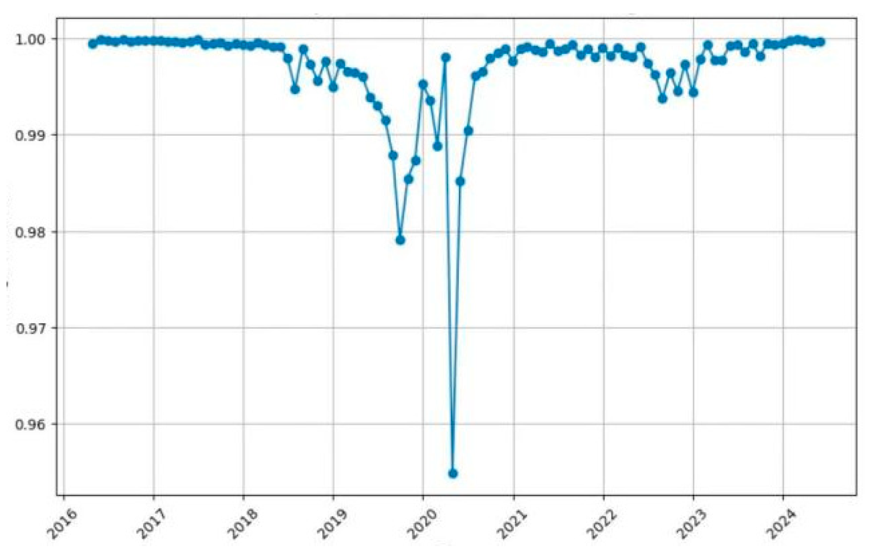
4.1. Global Financial Market Risk Index Analysis

Take G20 as the research object. Considering that the economic and financial policies of the Chinese mainland, Hong Kong, Macao, and Taiwan are relatively independent of each other, and Macao, China has no independent stock market, this paper divides China into three samples: the Chinese mainland, Hong Kong, and Taiwan. At the same time, because the exchange rate level and foreign exchange reserves involved in this paper are linked to the US dollar, the US sample is excluded. The EU is also excluded. According to the availability of data, this paper selected monthly data on interest rate levels, foreign exchange reserves, and currency exchange rates, levelled against the US dollar, from the CEIC database and stock market closing price data from Investing.com for all countries (regions) from January 2016 to May 2024. After a calculation using the above risk index formula, this paper obtained the monthly money market risk index, foreign exchange market risk index, and stock market risk index from February 2016 to May 2024 for 20 countries (regions), and then added these up to obtain the financial market risk index.

Figure 1 ranks the annual average risk index of 20 financial markets, showing two obvious echelons on the whole. The average risk index for the 17 countries (regions) from South Korea to Türkiye is around 0.4–0.5, while the Chinese mainland, Japanese, and Taiwanese indices are around 0.15. From the perspective of the countries (regions), Türkiye exhibits the highest average risk index among them. World Bank and IMF data show that between 2016 and 2024, its economy was plagued by political instability, with frequent policy changes and geopolitical tensions. This led to a large current account deficit, averaging about 3.6% of GDP, making it highly reliant on foreign capital. Moreover, its foreign exchange reserves were insufficient to cover short-term external debt, with the ratio often below the international safety threshold of one. Argentina follows closely in terms of risk. Official inflation data indicate an average annual inflation rate exceeding 30%, during this period. By the end of 2023, its external debt had reached around USD 266.17 billion, forcing it to frequently borrow from international financial institutions. The peso depreciated significantly, with an average annual depreciation of about 38% against the US dollar from 2016 to 2024. Conversely, the average risk index in East Asia was smaller overall, with South Korea, Taiwan, Japan, and the Chinese mainland all at the back. Among them, the Chinese mainland has the lowest average risk index, mainly because of China’s large economic scale, strong government intervention capacity, and stable political environment. The Chinese government has strong control capabilities in the economic and financial fields, and can take active policy measures to stabilize the market and deal with risks. For example, during the 2008 global financial crisis and the 2020 COVID-19 pandemic, China’s swift implementation of large-scale economic stimulus packages and targeted financial policies stabilized the market more effectively than some Western countries with less coordinated policy responses. These measures, combined with China’s substantial foreign exchange reserves, stable exports, and low foreign debt levels, provide stronger safeguards for financial stability. In contrast, some Western countries faced difficulties in policy coordination and market stabilization due to political and institutional constraints.

To assess the robustness of the model, we initially attempted to recalculate the weights using a Principal Component Analysis, but this was not applicable due to a failure in the KMO test. We sought additional evidence from relevant studies to support the reliability of this practice. On the one hand, Illing and Liu (2003) constructed Canada’s comprehensive financial pressure index based on the factor analysis method, equal variance weight method, and credit weight method, respectively [3]. It was found that the correlation coefficient between the pressure index obtained by the factor analysis method and the index obtained by the other three methods was not high, while the error rate of the credit weight method was the lowest. On the other hand, Balakrishnan et al. (2009) [33] referred to the fact that previous studies have shown that using the inverse of the standard deviation as the weight in some countries is similar to the weight determined by the corresponding principal component analysis. They also stated that, despite the fact that the composite index should ideally use economic indicators such as credit, such weights lack a cross-national and comparable basis. Given the need for further research into the risk relationships among countries, we finally believe that the selected models are reliable to some extent.

4.2. Analysis of Fluctuation Spillover Effects and Correlation Network in Global Financial Markets

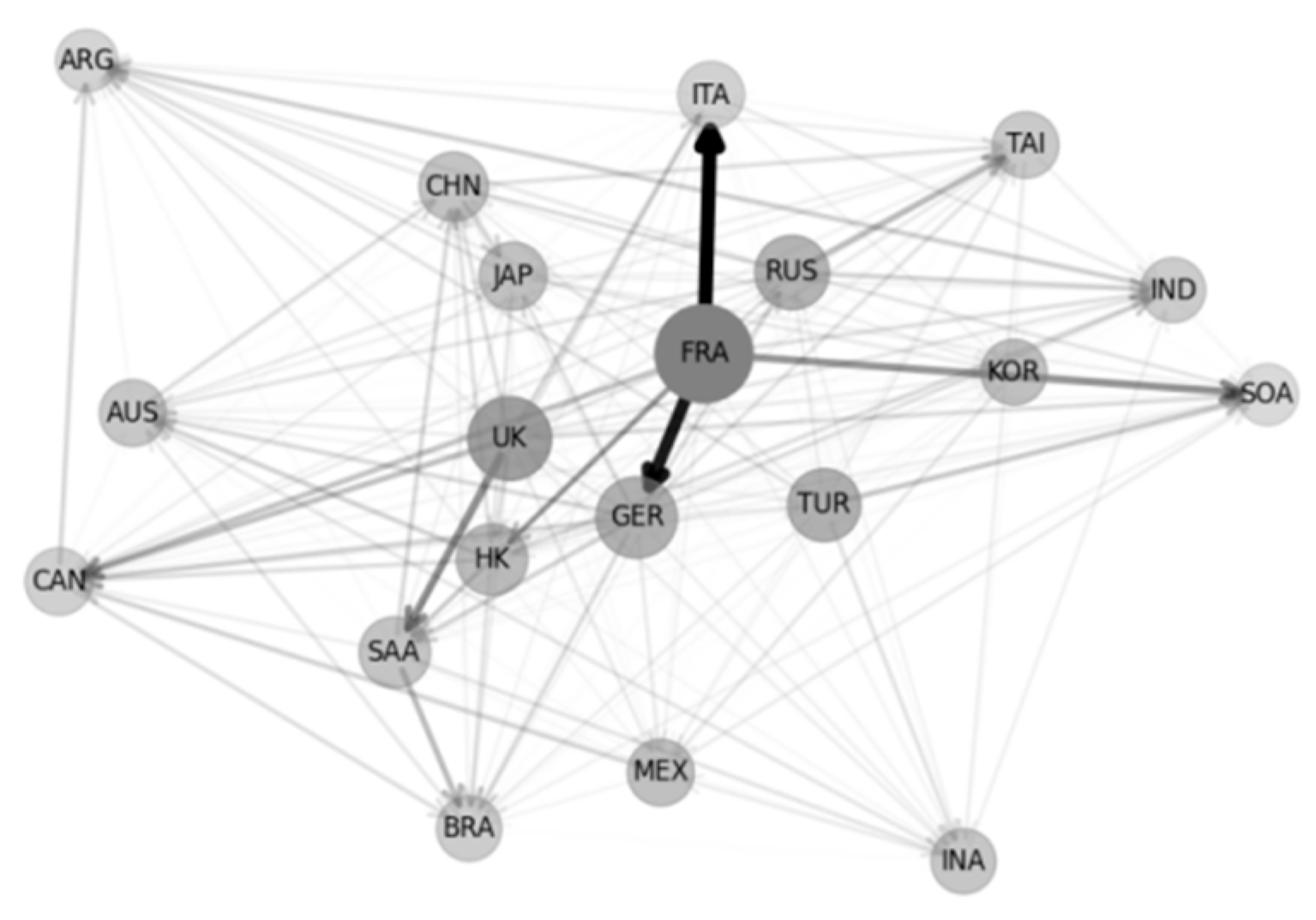
4.2.1. Analysis of the Overall Fluctuation Spillover Effect of the Financial Market and the Correlation Network

In order to pass the unit root test and the VAR model stationarity test, this paper first establishes the first order difference of the data. Then, the vector autoregression model and prediction error variance decomposition are used to obtain the spillover effect matrix of financial market fluctuations. Based on this,

Table 1. Volatility effects of global financial markets.

RANK	Country	NET	RATE	OUT	IN	GROSS	E	RANK	Country	NET	RATE	OUT	IN	GROSS	E
1	FRA	187.26	44.25	223.40	36.13	259.53	72.16	11	SAA	−13.01	3.07	55.95	68.96	124.91	10.41
2	UK	98.14	23.19	142.74	44.60	187.34	52.39	12	INA	−19.04	4.50	33.69	52.74	86.43	22.03
3	TUR	47.20	11.15	74.57	27.37	101.94	46.30	13	AUS	−22.75	5.38	47.83	70.58	118.41	19.21
4	GER	41.31	9.76	123.11	81.80	204.91	20.16	14	TAI	−28.41	6.71	45.12	73.53	118.65	23.94
5	RUS	37.26	8.81	85.11	47.84	132.95	28.03	15	BRA	−37.07	8.76	28.96	66.02	94.98	39.02
6	HK	12.01	2.84	83.97	71.96	155.93	7.70	16	IND	−38.80	9.17	36.45	75.25	111.71	34.73
7	KOR	−2.62	0.62	45.45	48.07	93.53	2.80	17	CAN	−49.57	11.71	44.64	94.21	138.85	35.70
8	MEX	−2.81	0.66	55.38	58.20	113.58	2.48	18	ITA	−53.11	12.55	45.18	98.28	143.46	37.02
9	JAP	−5.68	1.34	61.33	67.01	128.33	4.42	19	ARG	−60.60	14.32	11.21	71.81	83.03	72.99
10	CHN	−11.71	2.77	66.39	78.09	144.48	8.10	20	SOA	−78.02	18.44	11.19	89.21	100.39	77.72

ranks the net risk spillover in each market, and shows the overflow, total amount, and transmission efficiency.

In terms of net risk spillover, there are more net exporting countries than net importing countries, which are mainly European countries. France is the largest exporter of net volatility spillover, with a net output of 187.26% to other global financial markets. Then came the UK, with a net output of 98.14%. The UK and France contributed more than 60 percent of their risk output, indicating their dominance in global volatility spillover. In addition, with the exception of Türkiye, Germany, Russia, and Hong Kong, the other 15 countries (regions) are all net importers of volatility spillover. Among them, mainland China’s net output in the 20 major financial markets is relatively balanced in terms of risk output and input levels. This shows that the Chinese mainland assumes a certain degree of risk in the financial markets and can effectively manage and control these risks. This balance helps to maintain the stability and sustainable development of financial markets and ensures the healthy operation of the financial system. At the same time, a balanced risk output and input can also help to reduce the volatility of financial markets and reduce the impact of financial risks on the entire economic system. Therefore, with the continuous improvement of China’s openness, China has a strong ability to control the ups and downs of the global financial market, which can allow it to effectively deal with the uncertain impact of potential financial risks in its economic operations.

Compared with some risk spillover indicators given in the table above, the risk transmission network can better show the pairwise corresponding directional spillover relationship and the relative status of different financial markets in risk conduction. Therefore, we use the global financial market risk transmission network G (N, E, W) shown in Figure 2 to obtain more information. Figure 2 illustrates the risk transmission network in the global financial market. The network diagram provides a visual representation of the pairwise corresponding directional spillover relationships and the relative status of different financial markets in risk conduction. In this network diagram, the nodes represent different financial markets, and the directed edges between them indicate the spillover effects of risk transmission from one market to another. The thickness of each edge corresponds to the magnitude of the risk spillover, while the direction of the edges indicates the direction of risk flow. The deeper the node color is, the greater the risk overflow ability. Additionally, the closer a node is to the geometric center of the network, the greater the degree centrality, and the higher its importance and influence in the network is, while the pointing and thickness of an edge indicate the direction and strength of the net risk overflow.

In terms of influence, the established financial powers such as France, Germany, and the UK are clearly at the center of the network and play a vital role in the global financial markets. When financial markets fluctuate, their risks are easier to pass on to each other, and the high connectivity and strong interaction of the financial transmission processes indicate that the financial market interdependence between these countries is very high. Among them, France serves as the strongest source of risk exports, and its financial market fluctuations have a profound impact on many countries or regions, while Germany and the UK are relatively significant in both output and input risks, playing an important intermediary role in the risk transmission network of the global financial market.

Russia, Japan, the Chinese mainland, and Hong Kong are at the subcenter of the network and still have some influence in the global market. The peripheral positions of the network are mainly filled by Argentina, Indonesia, and Canada, indicating that they have relatively little influence in risk transmission. But they are still in touch with multiple core nodes, and their markets’ stability has a certain impact on risk transmission in the global financial market. In terms of influence, the interaction between the three EU countries is very significant. The thickest and deepest arrows point from France to Italy, Germany, and South Africa, and from the UK to Saudi Arabia, indicating that the risk transmission of these connections in financial markets is extremely significant.

4.2.2. Market Volatility Spillover Effect and Correlation Network Analysis

The above method is also used to study the spillover effect of financial markets, money markets, foreign exchange markets, and stock markets.

Table 2. Spillover effect of market fluctuations in global financial markets. Since the European Union adopts a unified currency, this paper refers to the unified currency market of France, Germany, and Italy as the EU currency market.

Category	Total Overflow Index	Country	UK	EUR			RUS	TUR	SAA	CHN	HK	TAI
				FRA	GER	ITA
money market	52.81	NET	78.53	72.02			74.98	32.62	37.52	−3.89	16.43	−37.9
		RATE	22.75	20.87			21.72	9.45	10.87	1.13	4.76	10.98
exchange market	70	NET	202.38	50.52	46.04	−1.24	25.71	45.48	21.7	36.37	20.82	−15.44
		RATE	45.07	11.25	10.25	0.28	5.73	10.13	4.83	8.1	4.64	3.44
stock market	77.05	NET	408.55	36.25	8.41	−50.87	22.42	0.55	−18.65	20.28	97.34	−44.37
		RATE	68.8	6.1	1.42	8.57	3.77	0.09	3.14	3.42	16.39	7.47
Category	Total Overflow Index	Country	JAP	KOR	IND	INA	AUS	CAN	MEX	BRA	ARG	SOA
money market	52.81	NET	−10.57	30.8	−42.46	−7.37	−14.13	−57.57	2.25	−34.91	−57.26	−79.09
		RATE	3.06	8.92	12.3	2.14	4.09	16.68	0.65	10.11	16.59	22.92
exchange market	70	NET	−13.23	−43.78	−47.47	−35.39	−25.41	−20.52	−58.65	−60.06	−55.76	−72.07
		RATE	2.95	9.75	10.57	7.88	5.66	4.57	13.06	13.37	12.42	16.05
stock market	77.05	NET	−9.57	−10.49	−34.84	−21.11	−70.02	−62.35	−69.28	−52.81	−76.69	−72.74
		RATE	1.61	1.77	5.87	3.56	11.79	10.5	11.67	8.89	12.91	12.25

and Figure 3 together show the volatility spillover effects of the three sub-markets of financial markets. The Figure 3a–c represents the risk transmission networks of a money market, foreign exchange market, and stock market, respectively. Each network diagram uses nodes to represent the individual sub-markets, and the edges between them show the risk spillover relationships within each specific sub-market. The color intensity and thickness of the edges highlight the strength of the spillovers within the respective markets. These figures provide a detailed view of the spillover effects within each sub-market and their interconnections.

From the perspective of the total market spillover index, the risk output level of the currency, foreign exchange, and stock markets increased successively, indicating that among the G20 countries (regions), the money market risk is the least stable, followed by the foreign exchange market, while the stock market has the greatest risk and is the most unstable. From the perspective of the market, the net risk output of the currency market and the number of net importing countries (regions) are equal and risk transmission is relatively average, wherein the UK, the EU, and Russia are mainly in the net risk overflow category, with more than 60% of the total risk output. In the foreign exchange market, the UK net risk spillover is close to 50% of the total, and the number of overall net risk exporters is less than that of net importers. The UK exhibits a net risk spillover of nearly 70% in the stock market, with a particularly strong risk export capacity, and then Hong Kong accounts for only 16%. From a national (regional) perspective, the UK, France, Germany, Türkiye, and Hong Kong are all in a net risk spillover role in all markets, while the UK is particularly evident in terms of net risk spillover performance, being the country with the largest net risk output in each market. Conversely, there are more countries (regions) in the net risk inflow role in all markets, with South Africa having the largest net risk input in each market.

The further analysis was expanded by the network graph. In the money market, the three EU countries and the UK are at the center of the network and have an important position in the risk transmission of the money interest rate market. In terms of influence relations, the risk transmission of the currency interest rate of Taiwan, China to South Africa and Russia is extremely significant. In the foreign exchange market, the UK is at the center of the network, the Chinese mainland, Italy, Türkiye, and Germany are at the subcenter, but the most obvious impact is France’s foreign exchange risk export to Italy. In the stock market, the countries at the center of the network are more dense, indicating that the risk transmission ability of the market is stronger. The UK is still at the main center of this network and is the leading exporter of risks, mainly to Australia, South Africa, and Canada.

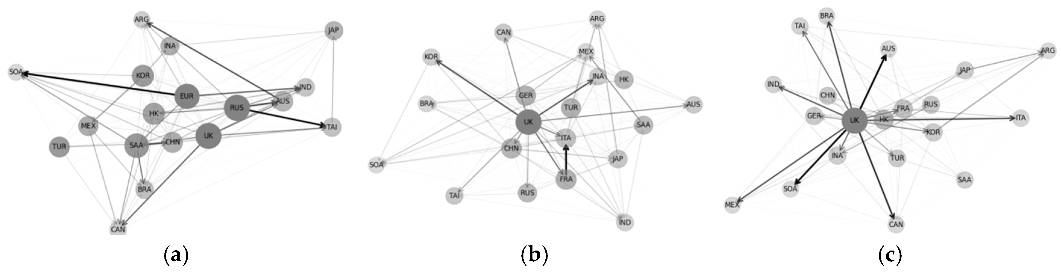
4.2.3. Cross-Market Volatility Spillover Effects and Correlation Network Analysis

We also select the sub-markets of countries (regions) with a strong risk transmission ability in each financial market as the main global financial markets to study the spillover effect of cross-market fluctuations.

Table 3. The spillover effect of the global financial market and cross-market fluctuations.

Rank	Market	NET	RATE	OUT	IN	GROSS	E	Rank	Market	NET	RATE	OUT	IN	GROSS	E
1	C_EUR	59.03	13.95	95.51	36.49	259.53	44.72	12	E_UK	−2.65	0.63	46.27	48.92	95.19	2.78
2	S_UK	45.38	10.72	102.55	57.17	187.34	28.41	13	E_GER	−4.71	1.11	40.35	45.06	85.41	5.51
3	C_JAP	35.96	8.50	68.98	33.03	101.94	35.25	14	E_JAP	−5.27	1.24	71.22	76.49	147.70	3.57
4	C_CHN	29.49	6.97	79.67	50.18	204.91	22.71	15	E_RUS	−8.48	2.00	65.22	73.70	138.92	6.10
5	C_UK	20.20	4.77	69.00	48.80	132.95	17.15	16	S_RUS	−15.63	3.69	51.81	67.44	119.25	13.11
6	E_HK	17.15	4.05	53.58	36.43	155.93	19.05	17	E_CHN	−30.52	7.21	48.84	79.37	128.21	23.81
7	E_FRA	11.45	2.71	72.82	61.36	93.53	8.54	18	S_HK	−35.71	8.44	46.56	82.27	128.83	27.72
8	C_HK	9.65	2.28	66.14	56.50	113.58	7.87	19	S_JAP	−36.65	8.66	27.49	64.14	91.63	40.00
9	C_RUS	8.93	2.11	64.34	55.41	128.33	7.46	20	E_KOR	−46.61	11.01	34.25	80.86	115.11	40.49
10	S_CHN	5.57	1.32	43.70	38.12	144.48	6.81	21	S_KOR	−59.01	13.94	29.27	88.28	117.55	50.20
11	C_KOR	2.44	0.58	50.75	48.32	99.07	2.46

and Figure 4 together show the details of the spillover effects across market fluctuations. Figure 4 illustrates the cross-market risk transmission network diagram, in which the circular nodes represent the money market, the square nodes represent the foreign exchange market, and the hexagonal nodes represent the stock market. This figure provides a comprehensive view of the spillover effects across different financial markets, highlighting the net risk output and input relationships between various markets. Overall, the net risk output market and the net risk input market are relatively equal, and the net risk output or net input of each market are relatively average. Among them, the markets with the strongest net risk output capacities are the EU money market and the UK stock market, while the main net risk input markets are the Korean stock market and the foreign exchange market.

In general, European countries such as the UK, France, and Germany are generally strong economically, while Brazil, Argentina, and South Africa are generally weak. First of all, there is heterogeneity in global financial markets, with different sizes, structures, and levels of development. As a result, the degree of correlation between financial markets cannot be determined by simple geographical distance. There are different financial systems and policies within and between different countries (regions), including monetary policies, exchange rate policies, interest rate policies, etc. These factors may lead to the weak spatial correlation of the global financial market. In addition, geopolitics is also one of the important factors. Geopolitical factors, such as trade wars, sanctions, and other political events, may cause significant differences among countries in the global financial markets, which may lead to large fluctuations and increased uncertainty in the financial markets of some countries (regions).

4.3. The Spatial and Temporal Characteristics of Risk Correlation in the Global Financial Markets

The above analysis focuses on the risk transmission relationship of the financial markets of various countries (regions). The following will further investigate the risk correlation of global financial markets from an overall perspective based on the time-varying characteristics and spatial characteristics of the global financial market association. To provide a more rigorous analysis of the factors influencing the variation of risk, we explore several key factors that drive these changes, including macroeconomic conditions, policy uncertainty, geopolitical events, and market participant behavior.

4.3.1. The Time-Varying Characteristics of the Global Financial Market Correlation

We explore the time-dependent characteristics of the global financial market correlation based on the time-dependent vector autoregressive model, and describe the average correlation degree of the global financial market with the monthly market risk, as shown in Figure 5. Figure 5, spanning from 2016 to 2024, shows the time-varying chart of the global financial market correlation. The vertical axis represents the average correlation degree, which ranges from 0.96 to 1.00, and the horizontal axis depicts the timeline by year. Each blue dot on the chart corresponds to the average monthly market correlation value. The figure illustrates the average degree of correlation of the global financial market with the monthly market risk, highlighting the periods of stability and fluctuation in relation to market correlation. Periods such as the end of 2019 and early 2020 display significant fluctuations, noticeable by the deviation of dots away from the value of one, indicating increased market instability. Thicker clusters of points near the value of one indicate periods of relative market stability with a higher correlation, whereas sparse and more volatile sections showcase the periods of fluctuation. The global financial market as a whole is more correlated, falling between 0.95 and 1. Among them, the correlation degree between 2016 and mid-2018 and mid-2023 and 2024 is relatively stable, around one, indicating that the connection between the financial markets is very close, showing a high degree of synchronization.

From the third quarter of 2018 to the third quarter of 2019, the market correlation began to decline slightly and then became increasingly large. The relevance of financial markets can be influenced by many factors, including macroeconomic conditions such as economic growth rates and inflation levels, trade policy, economic growth prospects, and geopolitical risks. Specifically, US President Donald Trump announced additional tariffs on imported steel and aluminum products in March 2018, and then imposed additional tariffs on some Chinese imports in July of the same year, which had a certain negative impact on the global financial market. Therefore, at this time, major international conflicts mainly existed between China and the United States, while the degree of association between the samples studied here decreased. As the trade war between China and the United States worsened, various tariffs and trade restrictions disrupted global supply chains, so the correlation of global financial markets declined further and further in 2019. In addition, in 2019, geopolitical risks in some parts of the world, such as tensions in the Middle East and the uncertainty caused by Brexit, all had an impact on market sentiment and investment behavior, as well as the volatility of the correlation of financial markets.

Since the first quarter of 2020, the correlation degree of global financial markets plummeted to the lowest level after a short period of time, indicating that the links between financial markets weakened sharply. This drastic change may be due to abnormal market fluctuations caused by sudden global events (such as COVID-19). Different markets had different degrees of impact and response speed to the epidemic, and market links were broken and fluctuated. During the outbreak, some countries (regions), including the sample countries Brazil, India, and Argentina, imposed capital controls or restricted capital flows to cope with financial market turmoil and foreign exchange fluctuations. Such measures could have weakened the links between global financial markets. In addition, investor sentiment and risk aversion behavior during the pandemic led investors to seek safe assets rather than pursuing high-risk and high-return investments, which could also have led to a weak correlation between the global financial markets.

Then, market correlation picked up, probably because the globally coordinated fiscal and monetary policies worked. During the recovery period, the gradual unsealing of countries (regions) and the recovery of economic activity, as well as the development and popularization of vaccines likely impacted this trend. After 2021, the correlation of global financial markets gradually stabilized; although there are small fluctuations, the overall curve is closer to a smooth curve. This means that the market gradually normalized after severe disruption, restabilizing and synchronizing.

4.3.2. Spatial Characteristics of the Global Financial Market Correlation

The Moran Index was used to test the global spatial autocorrelation of the whole financial market and the sub-markets from 2016 to 2024. The results are shown in

Table 4. Global autocorrelation Moran index. *** p < 0.01, ** p < 0.05, * p < 0.1.

	2016	2017	2018	2019	2020	2021	2022	2023	2024
FRM	−0.135 ***	−0.134 ***	−0.135 ***	−0.136 ***	−0.136 ***	−0.134 ***	−0.131 ***	−0.136 ***	−0.133 ***
CRM	−0.115 ***	−0.045	−0.074	−0.068	−0.075	−0.062	−0.042	−0.095 **	−0.071
ERM	−0.067 **	−0.069 **	−0.066	−0.076	−0.096 **	−0.089 *	−0.101 **	−0.015 *	−0.083
SRM	−0.078	−0.081 *	−0.077	−0.079	−0.081 *	−0.081 *	−0.082 *	−0.082 *	−0.085 *

. All coefficients are negative, indicating that there may be spatial characteristics of discrete distribution in each market. Based on the p-value, the financial market as a whole has passed the significance level of 1%, but the coefficients are close to 0, indicating that although it could be considered a significant discrete distribution in the financial market, the degree of dispersion is very small. In addition, the Moran indices of the currency market, foreign exchange market, and stock market do not pass the significance level of 10% every year and their coefficients are also close to 0. The negative and near-zero Moran index values suggest a weak spatial autocorrelation in the global financial market. This indicates that the financial risks are not strongly clustered in specific regions, but rather are more evenly distributed across the globe. This result is important because it suggests that global financial markets are not significantly influenced by geographical proximity, which is a key finding for understanding the spatial dynamics of financial risk transmission. The weak spatial autocorrelation implies that financial risks may be more influenced by other factors, such as global economic conditions, trade relationships, and geopolitical events, rather than by the physical distance between markets. The statistical significance of the Moran index was tested using a p-value approach. The p-values for the overall financial market Moran index were below the 1% significance level, indicating that the observed spatial distribution is statistically significant. However, the small magnitude of the Moran index coefficients suggests that the spatial autocorrelation is weak. Confidence intervals for the Moran index were also calculated to provide a range within which the true Moran index is likely to fall. These intervals further support the conclusion that the spatial autocorrelation is weak but statistically significant.

Although geographical distance may affect the connection between financial markets, the influence of globalization and information technology on the correlation between global financial markets is gradually weakened. Multi-national financial institutions operate on a global scale and can flow and trade funds between different countries. In addition, with the popularization and development of the Internet and communication technology, the information transmission speed in financial markets has become faster, and investors can have more convenient access to global market information. To further explore the reasons behind the weak spatial correlation of risk transmission, we consider the combined effects of high capital mobility, the limited impact of trade restrictions, and divergent monetary policies. High capital mobility allows financial risks to spread quickly and widely, reducing the clustering effect of the risks in specific regions. While trade restrictions can impact economic activity, their effect on financial risk transmission may be limited, as financial markets are often more responsive to global economic conditions and investor sentiment. Additionally, divergent monetary policies among countries can lead to varied responses to financial risks, further reducing the synchronization of financial market movements and weakening the spatial correlation of risks. These factors collectively contribute to a more dispersed distribution of financial risks across the globe.

Table 5. Local autocorrelation Moran index. *** p < 0.01, ** p < 0.05, * p < 0.1.

2016	H-H	L-H	L-L	H-L	2018	H-H	L-H	L-L	H-L
FRI		CHN **	TAI ***		FRI		CHN **	TAI ***
CRI		JAP **	TAI ***	MEX **	CRI		GER ** ITA *		CHN ***
ERI	TAI ***			CHN ***	ERI
SRI		ARG ***			SRI		ARG ***
2021	H-H	L-H	L-L	H-L	2024	H-H	L-H	L-L	H-L
FRI		CHN **	TAI ***		FRI		CHN **	TAI ***
CRI	BRA *** KOR *	ITA *		CHN ***	CRI				JAP **
ERI					ERI	RUS *	MEX **
SRI		ARG ***			SRI		ARG ***

shows the local spatial autocorrelation of the financial market in G20 countries (regions), which is generally insignificant in most countries (regions). In the financial market as a whole, the Chinese mainland is in the L-H cluster, where its own financial market risk is low but the risk is high for the surrounding markets, while Taiwan, China is in the L-L cluster, where its own and the surrounding financial market are low-risk. In the money market, Italy was in the L-H cluster in 2018 and 2021, and the Chinese mainland was in the H-L cluster, indicating that Italy’s money market risk is lower than that of neighboring countries, while for the Chinese mainland it is exactly the opposite. In addition, in the foreign exchange market, Taiwan, the Chinese mainland, and four other countries (regions) have only seen one significant local autocorrelation in different years; while in the stock market, Argentina is in the L-H cluster every year, where the risk is significantly lower than in the surrounding markets. In general, the Chinese mainland and Taiwan have a significant and sustained local autocorrelation in the financial market, as well as having a similar correlation with Argentina in the stock market. While seven countries, including Japan and Italy, have occasionally seen local autocorrelation in some markets in some years, the other 10 countries (regions) do not have local autocorrelation.

5. Conclusions

This paper examines the global financial market from 2016 to 2024 using data from the G20 countries (regions) as samples. It focuses on three market risk indices and employs risk spillover matrices and network analysis methods to analyze the overall financial market, as well as the relationships between market and cross-market risk transmission. This study uncovers the complex structure and evolving trends of the global financial market.

During the research period, the financial market risk index of the G20 countries (regions) showed two obvious echelons on the whole. Türkiye has the highest average risk index, while the Chinese mainland has the lowest average risk index. In analyzing volatility spillovers, France emerges as the largest net exporter in the financial market, while the UK exhibits a stronger spillover capacity in the currency and stock markets; in the cross market, the net outputs or net inputs of each market are relatively average, but with the EU currency market and the UK currency market as the primary spillover markets still. Overall, the UK, France, and Germany have strong net spillover capacities in relation to volatility, while Argentina’s and South Africa’s are weak. Additionally, we found that the risk associations in the G20 financial markets show significant time-varying characteristics, with correlation fluctuations observed during a trade war and the COVID-19 pandemic. However, the spatial characteristics reveal a weakly discrete distribution, where mainland China’s and Taiwan’s markets are in the L-H and L-L clusters, respectively, and Argentina’s stock market consistently falls into the L-H cluster.

These findings align with and extend the existing literature. For instance, our identification of the strong net spillover capacity of major economies such as that of the UK, France, and Germany corroborates the observations made by Billio et al. (2012) and Diebold and Yilmaz (2009), who emphasized the significant role of interconnectedness in financial markets [14,17]. However, our study goes beyond their work by incorporating a spatial–temporal analysis, which is a significant advancement over previous research. Unlike Zhao et al. (2018), who analyzed the risk spillover effect of global foreign exchange market pressure but did not consider the spatial–temporal dynamics [41], our research captures the complex interdependencies and time-varying characteristics of financial risks across multiple markets. This comprehensive approach not only enriches the existing literature but also offers practical insights for policymakers aiming to enhance global financial stability.

Based on the above research conclusions, we suggest that countries should enhance international cooperation, particularly those with a significant net spillover capacity such as France, the UK, and Germany, to establish multilateral financial stability mechanisms and strengthen the monitoring and early warning of cross-market and cross-border risks. Countries should also optimize their domestic economic policies to maintain stable economic growth and reduce the negative impact of economic fluctuations on financial markets. Additionally, policymakers should develop adaptive emergency response strategies to address the impact of emergencies on the market, considering the time-varying characteristics of financial market risks.

For high-risk and emerging economies such as those of Türkiye and Argentina, targeted strategies should be implemented to mitigate financial risks. These countries should prioritize strengthening their foreign exchange reserves to enhance economic stability and reduce vulnerability to external shocks. Implementing structural reforms to enhance economic efficiency and resilience is also crucial. Diversifying export markets can help reduce dependence on a limited number of trading partners, while improving fiscal discipline ensures sustainable public finances and effective management of debt levels. Prioritizing debt restructuring can stabilize currency and reduce the burden of external debt. Promoting economic diversification can attract foreign direct investment and reduce dependency on volatile external financing. These measures can help high-risk and emerging economies better manage their financial risks and contribute to the overall stability of the global financial system.

For developed economies such as those of the UK and France, strategies to reduce the impact of spillover could include enhancing financial regulatory frameworks to ensure a robust oversight of financial institutions. Promoting international cooperation to coordinate policies and share information on financial market risks is essential. Establishing multilateral financial stability mechanisms can strengthen the monitoring and early warning of cross-market and cross-border risks. Implementing sound monetary and fiscal policies can stabilize domestic financial markets and reduce the negative impact of economic fluctuations on other countries. Improving the resilience of their financial systems can mitigate the transmission of financial shocks. By taking these measures, developed economies can play a more constructive role in maintaining global financial stability.

References

1. Panazan, O.; Gheorghe, C. Impact of geopolitical risk on G7 financial markets: A comparative wavelet analysis between 2014 and 2022. Mathematics 2024, 12, 370. [Google Scholar] [CrossRef]
2. Yang, Z.H.; Chen, Y.T.; Zhang, P.S. Research on the cross-market contagion of tail risks in stock and foreign exchange markets. J. Manag. Sci. China 2020, 23, 54–77. [Google Scholar]
3. Illing, M.; Liu, Y. An Index of Financial Stress for Canada (Bank of Canada Working Paper 2003-14); Bank of Canada: Ottawa, ON, Canada, 2003. [Google Scholar]
4. Stiglitz, J.E. Risk and Global Economic Architecture: Why Full Financial Integration May Be Undesirable. Am. Econ. Rev. 2010, 100, 388–392. [Google Scholar] [CrossRef]
5. Allen, F.; Gale, D. Financial Contagion. J. Political Econ. 2000, 108, 1–33. [Google Scholar] [CrossRef]
6. Baker, M.; Wurgler, J. Investor Sentiment and the Cross-Section of Stock Returns. J. Financ. 2006, 61, 1645–1680. [Google Scholar] [CrossRef]
7. Engle, R.F. Dynamic Conditional Correlation: A Simple Class of Multivariate GARCH Models. J. Bus. Econ. Stat. 2002, 20, 339–350. [Google Scholar] [CrossRef]
8. Forbes, K.J.; Rigobon, R. No Contagion, Only Interdependence: Measuring Stock Market Comovements. J. Financ. 2002, 57, 2223–2261. [Google Scholar] [CrossRef]
9. Patton, A.J. Modelling Asymmetric Exchange Rate Dependence. Int. Econ. Rev. 2006, 47, 527–556. [Google Scholar] [CrossRef]
10. Cai, J.; Cheung, Y.L.; Wong, M.C.S. What Moves the Gold Market? J. Futur. Mark. Futures Options Other Deriv. Prod. 2009, 29, 491–507. [Google Scholar] [CrossRef]
11. Dixon, L.; Clouse, C.; McCulloch, J. The Relationship Between Financial Market Liquidity and International Transmission of Financial Shocks. J. Int. Money Financ. 2017, 74, 227–242. [Google Scholar]
12. Bekaert, G.; Harvey, C.R.; Lundblad, C. Financial Openness and Productivity. World Dev. 2014, 52, 31–50. [Google Scholar]
13. Dungey, M.; Fry, R.; González-Hermosillo, B.; Martin, V.L. Empirical Modeling of Contagion: A Review of Methodologies. Quant. Financ. 2005, 5, 9–24. [Google Scholar] [CrossRef]
14. Billio, M.; Getmansky, M.; Lo, A.W.; Pelizzon, L. Econometric Measures of Connectedness and Systemic Risk in the Finance and Insurance Sectors. J. Financ. Econ. 2012, 104, 535–559. [Google Scholar] [CrossRef]
15. Bollerslev, T. Generalized Autoregressive Conditional Heteroskedasticity. J. Econom. 1986, 31, 307–327. [Google Scholar] [CrossRef]
16. Brunnermeier, M.K.; Crocket, A.; Goodhart, C.; Persaud, A.D.; Shin, H. The Fundamental Principles of Financial Regulation; International Center for Monetary and Banking Studies: Geneva, Switzerland, 2009. [Google Scholar]
17. Diebold, F.X.; Yilmaz, K. Measuring Financial Asset Return and Volatility Spillovers, with Application to Global Equity Markets. Econ. J. 2009, 119, 158–171. [Google Scholar] [CrossRef]
18. Lanne, M.; Saikkonen, P. Noncausal Vector Autoregression. J. Appl. Econom. 2011, 26, 636–664. [Google Scholar]
19. Caporin, M.; McAleer, M.; Zekaite, Z. Exchange Rate Volatility and Risk Spillovers in Global Financial Markets. Int. Rev. Econ. Financ. 2018, 56, 56–77. [Google Scholar]
20. Caporin, M.; Pelizzon, L.; Ravazzolo, F.; Rigobon, R. Measuring Sovereign Contagion in Europe. J. Financ. Stab. 2018, 34, 150–181. [Google Scholar] [CrossRef]
21. Lau, W.Y.; Go, Y.H. Dynamic causality between stock return and exchange rate: Is stock—Oriented hypothesis more relevant in Malaysia? Asia—Pac. Financ. Mark. 2018, 25, 137–157. [Google Scholar] [CrossRef]
22. Maitra, D.; Dawar, V. Return and volatility spillover among commodity futures, stock market and exchange rate: Evidence from India. Glob. Bus. Rev. 2019, 20, 214–237. [Google Scholar] [CrossRef]
23. Zhao, Y.P.; Qin, L.S.; Huang, Y.X. Research on the risk spillover effect of global foreign exchange market pressure: Based on spillover index and network topology analysis. World Econ. Study 2020, 8, 3–16+135. [Google Scholar]
24. Xiao, Y.X.; Li, X.Y. Research on the spillover effect between the foreign exchange market and the stock market—Analysis based on the W-VAR-MGARCH-BEKK model. South China Financ. 2014, 2, 59–64. [Google Scholar]
25. Li, L.; Wang, B.; Hao, D.P. Central Bank’s Exchange Rate Communication and Stock Market Volatility. Financ. Forum 2019, 24, 52–66+80. [Google Scholar]
26. Yu, B.; Guan, C.; Dai, S.G. Research on the linkage of financial markets across the Taiwan Strait and in Hong Kong—Based on the six—Element asymmetric VAR—BEKK—MVGARCH model. Asia—Pac. Econ. Rev. 2019, 4, 136–142. [Google Scholar]
27. Zhou, B.C.; Zhang, H.; Cao, Q. Industry heterogeneity of the volatility spillover effect between RMB exchange rate and stock market. Tax. Econ. 2021, 5, 55–61. [Google Scholar]
28. Chen, G.J.; Xu, D.X.; Chen, J. Analysis of the volatility spillover effect between China’s stock market and foreign exchange market. J. Quant. Tech. Econ. 2009, 26, 109–119. [Google Scholar]
29. He, C.Y.; Liu, L.; Xu, X.Y. Foreign exchange market intervention, exchange rate changes and stock price volatility—Theoretical model and empirical research based on investor heterogeneity. Econ. Res. J. 2013, 48, 29–42+97. [Google Scholar]
30. Chen, Y.; Chen, L.N.; Lin, L.D. Research on the volatility spillover effect between RMB exchange rate and stock market. Manag. Sci. 2009, 22, 104–112. [Google Scholar]
31. Sachs, J.; Tornell, A.; Velasco, A. Financial Crises in Emerging Markets: The Lessons from 1995; Brookings Papers on Economic Activity; National Bureau of Economic Research: Cambridge, MA, USA, 1996; Volume 27, pp. 147–216. [Google Scholar]
32. Wang, C.L.; Hu, L. Research on early warning of China’s financial risks based on Markov regime switching model. J. Financ. Res. 2014, 40, 99–114. [Google Scholar]
33. Balakrishnan, R.; Danninger, S.; Elekdag, S.; Tytell, I. The Transmission of Financial Stress from Advanced to Emerging Economies (IMF Working Paper No. WP/09/133); International Monetary Fund: Washington, DC, USA, 2009. [Google Scholar]
34. Jiang, W.; Yu, Q.L. Carbon emissions and economic growth in China: Based on mixed frequency VAR analysis. Renew. Sustain. Energy Rev. 2023, 183, 113500. [Google Scholar] [CrossRef]
35. Dong, J.; Li, C. Structure characteristics and influencing factors of China’s carbon emission spatial correlation network: A study based on the dimension of urban agglomerations. Sci. Total Environ. 2022, 853, 158613. [Google Scholar] [CrossRef] [PubMed]
36. Liu, D.; Zeng, X.; Su, B.; Wang, W.; Sun, K.; Sadia, U.H. A social network analysis regarding electricity consumption and economic growth in China. J. Clean. Prod. 2020, 274, 122973. [Google Scholar] [CrossRef]
37. Mitze, T.; Strotebeck, F. Centrality and get-richer mechanisms in interregional knowledge networks. Reg. Stud. 2018, 52, 1477–1489. [Google Scholar] [CrossRef]
38. Antonakakis, N.; Chatziantoniou, I.; Gabauer, D. Refined Measures of Dynamic Connectedness based on Time-Varying Parameter Vector Autoregressions. J. Risk Financ. Manag. 2020, 13, 84. [Google Scholar] [CrossRef]
39. Alrweili, H.; Ben-Salha, O. Dynamic asymmetric volatility spillover and connectedness network analysis among sectoral renewable energy stocks. Mathematics 2024, 12, 1816. [Google Scholar] [CrossRef]
40. Tian, Y.; Wu, Y. Systemic financial risk forecasting: A novel approach with IGSA—RBFNN. Mathematics 2024, 12, 1610. [Google Scholar] [CrossRef]
41. Zhao, X.J.; Zhang, W.G.; Liu, Y.J. Volatility spillovers and risk contagion paths with capital flows across multiple financial markets in China. Emerg. Mark. Financ. Trade 2018, 56, 731–749. [Google Scholar] [CrossRef]
Figure 1. Annual average risk index of the G20 financial markets. The meanings of each code in the picture are as follows (the same below): CHN (China), JAP (Japan), TAI (Taiwan), KOR (Republic of Korea), INA (Indonesia), FRA (France), AUS (Australia), GER (Germany), IND (India), CAN (Canada), ITA (Italy), SOA (South Africa), SAA (Saudi Arabia), HK (Hong Kong), MEX (Mexico), BRA (Brazil), UK (The United Kingdom), RUS (Russia), ARG (Argentina), and TUR (Türkiye).
Mathematics 13 01353 g001
Figure 2. Risk transmission network diagram for global financial markets.
Mathematics 13 01353 g002
Figure 3. (a) Risk transmission network of money market. (b) Risk transmission network of foreign exchange market. (c) Risk transmission network of stock market.
Mathematics 13 01353 g003
Figure 4. Cross-market risk transmission network diagram.
Mathematics 13 01353 g004
Figure 5. Time-varying chart of global financial market correlation.
Mathematics 13 01353 g005