Finite Element Method for Solving the Screened Poisson Equation with a Delta Function

Abstract

This paper presents a Finite Element Method (FEM) framework for solving the screened Poisson equation with a Dirac delta function as the forcing term. The singularity introduced by the delta function poses challenges for standard numerical methods, particularly in higher dimensions. To address this, we employ integrated Legendre basis functions, which yield sparse and structured system matrices characterized by a Banded-Block-Banded-Arrowhead ($B^3$-Arrowhead) form. In one dimension, the resulting linear system can be solved directly. In two and three dimensions, the equation can be efficiently solved using a generalized Alternating Direction Implicit (ADI) method combined with reverse Cholesky factorization. Numerical results in 1D, 2D, and 3D confirm that the method accurately captures the localized impulse response and reproduces the expected Green’s function behavior. The proposed approach offers a robust and scalable solution framework for partial differential equations with singular source terms and has potential applications in physics, engineering, and computational science.

1. Introduction

The screened Poisson equation is a classical partial differential equation that arises in a wide range of scientific and engineering applications, including electrostatics, quantum mechanics, image processing, and signal analysis. In this study, we focus on solving the screened Poisson equation over a rectangular domain:

$$-\Delta u(x,y)+{\omega }^{2}u(x,y)=f(x,y)\mathrm{for}a\le x\le b,c\le y\le d$$

(1)

where $\Delta u:=u_{xx}+u_{yy}$ is the Laplacian and $\omega$ is a fixed parameter controlling the decay rate of the solution. A particular challenge arises when the forcing term $f(x,y)$ is modeled by a Dirac delta function $\delta (x,y)$, representing a localized impulse.

While Fortunato [1] proposed a fast spectral solver using the Alternating Direction Implicit (ADI) method with quasi-optimal complexity for continuous functions on right hand side, and Knook and Olver [2] extended these ideas to discontinuous function, the treatment of delta-function forcing remains nontrivial in practical computations.

In the paper, we aim to solve the screened Poisson equation in 1D, 2D, and 3D with respect to a delta function (generalized function), which plays an important role on mathematical analysis, physics, signal processing, engineering, and image processing. While standard finite element methods may face difficulties in resolving the localized singularity introduced by the delta function, this issue can be mitigated by carefully choosing the specialized basis functions. In this work, we adopt integrated Legendre functions originally introduced by Babuska and Suri [3] within the FEM framework. These functions exhibit highly sparse matrix structures when applied to the variational form of elliptic PDEs. Specifically, we exploit the resulting Banded-Block-Banded-Arrowhead ($B^3$-Arrowhead) structure to develop efficient discretizations for the screened Poisson equation in one, two, and three spatial dimensions.

Our approach combines theoretical developments with practical numerical techniques, including generalized and nested ADI [2,4], to maintain sparsity and computational efficiency. We conclude with visual demonstrations of the solution in 1D, 2D, and 3D, highlighting the structure of the Green’s function as a response to delta excitation.

The development of sparse FEM has an interesting history. The origins can be traced back to the research of Szabo and Babuska, with further elaborations found in [5,6]. Babuška and Suri [3] and Beuchler and Schoberl [7] expanded these methods to two dimensions, creating p-FEM for quadrilaterals and simplices, respectively. Additional contributions in this area include works by [5,8,9,10,11,12,13,14,15,16,17].

The main contributions of this paper are summarized as follows:

• We propose a finite element method using integrated Legendre basis functions to solve the screened Poisson equation with Dirac delta forcing, preserving sparsity and capturing singular behavior.
• We develop a structured discretization approach that leads to Banded-Block-Banded Arrowhead matrices, and apply it in 1D, 2D, and 3D domains.
• We employ and adapt the ADI method to efficiently solve the resulting systems.
• We present detailed numerical results that confirm the expected Green’s function behavior and validate the accuracy of our method for singular sources.

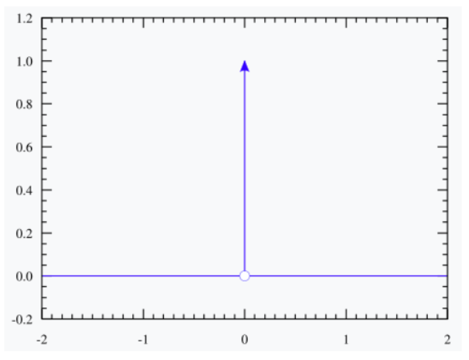
To the best of our knowledge, this is the first comprehensive application of this combined approach to delta-function forcing across multiple dimensions.

The remainder of this paper is organized as follows: Section 2 introduces the definition and properties of the delta function. Section 3 discusses integrated Legendre functions and their role in constructing sparse discretizations. Section 4 presents FEM formulations and numerical solutions in 1D, 2D, and 3D. Section 5 analyzes the computational cost. Finally, Section 6 concludes this paper with discussions and potential directions for future work.

2. Delta Function

Firstly, we need to knowthe definition and property of the delta function to obtain useful information in discretizations of the screened Poisson equation.

Figure 1 gives a clear function expression [18]. Next, we will present the rigorous definitions and properties [18].

2.1. Definitions

The dirac delta function $\delta (x)$ loosely is zero when x is not equal to zero, and it is infinite when x is equal to zero:

$$\delta (x)=\left\{\begin{array}{cc}\infty \hfill & x=0\hfill \\ 0\hfill & x\ne 0\hfill \end{array}\right.$$

and it satisfies the following:

$${\int }_{-\infty }^{\infty }\delta (x)dx=1.$$

2.2. As a Measure

Formally, the Lebesgue integral serves as the essential analytical tool. The integral, in the sense of Lebesgue, taken with respect to the measure $\delta$, satisfies the following:

$${\int }_{-\infty }^{\infty }f(x)\delta (dx)=f(0)$$

for all continuous compactly supported functions f. However, we often use the following:

$${\int }_{-\infty }^{\infty }f(x)\delta (x)dx=f(0).$$

This notation is a useful but an informal convention and does not represent a standard integral in the Riemann or Lebesgue sense.

2.3. Generalizations

In n-dimensional Euclidean space ${\mathbf{R}}^n$, the delta function can be characterized as a measure that satisfies the following:

$${\int }_{{\mathbf{R}}^n}f(\mathbf{x})\delta (d\mathbf{x})=f(\mathbf{0})$$

for any continuous function f with compact support. Viewed as a measure, the n-dimensional delta function is defined as the product of one-dimensional delta functions applied independently to each coordinate. Hence, given $\mathbf{x}=(x_1,x_2,\dots ,x_n)$, it can be formally expressed as follows:

$$\delta (\mathbf{x})=\delta (x_1)\delta (x_2)\cdots \delta (x_n).$$

3. Integrated Legendre Functions

We review integrated Legendre functions of [2,3] and explore their role in developing discretizations of differential operators with a unique sparsity structure known as Banded-Block-Banded Arrowhead Matrices.

3.1. A Set of Basis Functions Defined over a Interval

Writing the weighted ultraspherical polynomials as

$$W_k(x):={\displaystyle \frac{(1-x^2)C_k^{(3/2)}(x)}{(k+1)(k+2)}}$$

where $C_k^{(t)}$ are orthogonal in ${(1-x^2)}^{t-1/2}$ on $[-1,1]$ for $t>-1/2$, $t\ne 0$ and it is

$$C_k^{(t)}(x)={\displaystyle \frac{2^k{(t)}_k}{k!}}{x}^k+O(x^{k-1})$$

where ${(t)}_k=t(t+1)\cdots (t+k-1)$ is Pochammer Symbol [2,19].

Also, we know

$$W_k^{\prime }(x)=-P_{k+1}(x)$$

for the Legendre polynomials $P_k(x)\equiv C_k^{(1/2)}(x)$ [1,2]. We can say these functions are the integrals of Legendre polynomials; essentially, they are the integrated Legendre functions up to a constant factor. They are the same as the basis described by Schwab [5] and used by Fortunato and Townsend [1].

A useful way to demonstrate this relationship is by employing quasimatrices. These can be viewed as matrices that are continuous along the first dimension, or alternatively, as a row vector with its columns representing functions. Therefore, we have the following:

$$\begin{array}{cc}\hfill \mathbf{W}(x)& =\left[W_0(x),W_1(x),W_2(x),\dots \right],\mathbf{P}(x)=\left[P_0(x),P_1(x),P_2(x),\dots \right],\hfill \\ \hfill {\displaystyle \frac{\mathrm{d}}{\mathrm{d}x}}\mathbf{W}& =\mathbf{P}\underset{D_W^P}{\underbrace{\left[\begin{array}{cccc}0& & & \\ -1& & & \\ & -1& & \\ & & -1& \\ & & & \ddots \end{array}\right]}},\hfill \end{array}$$

where $\mathbf{W}(x)$ and $\mathbf{P}(x)$ are $1\times \infty$ row-vector. Also, we can view $\mathbf{W}$ and $\mathbf{P}$ as $[-1,1]\times \infty$ quasi-matrices.

For a single element in one dimension, this basis can serve as both the test and trial basis in the weak formulation of a differential equation. We denote the $L^2(-1,1)$ inner product by $\langle ·,·\rangle$. Consequently, the gram or mass matrix associated with Legendre polynomials is as follows:

$$\langle {\mathbf{P}}^{\top },\mathbf{P}\rangle :=\left[\begin{array}{ccc}\langle P_0,P_0\rangle & \langle P_0,P_1\rangle & \cdots \\ \langle P_1,P_0\rangle & \langle P_1,P_1\rangle & \cdots \\ ⋮& ⋮& \ddots \end{array}\right]=\underset{{\mathbf{M}}_P}{\underbrace{\left[\begin{array}{cccc}2& & & \\ & 2/3& & \\ & & 2/5& \\ & & & \ddots \end{array}\right]}}$$

While the discretization of the weak 1D Laplacian results in a diagonal matrix [2]:

$$\begin{array}{cc}\hfill -{\Delta }_W& :=\langle {({\mathbf{W}}^{\prime })}^{\top },{\mathbf{W}}^{\prime }\rangle =\langle {(\mathbf{P}{D}_W^P)}^{\top },\mathbf{P}{D}_W^P\rangle \hfill \\ \hfill & ={(D_W^P)}^{\top }{M}_P{D}_W^P=\left[\begin{array}{cccc}2/3& & & \\ & 2/5& & \\ & & 2/7& \\ & & & \ddots \end{array}\right].\hfill \end{array}$$

 And, we have alternative way to write the formula:

$$\langle W_k^{\prime },W_j^{\prime }\rangle =\langle P_{k+1},P_{j+1}\rangle ={\displaystyle \frac{2}{2k+3}}{\delta }_{kj}.$$

From [1,2], the mass matrix can be derived by utilizing the lowering relationship:   

$$\underset{\mathbf{W}}{\underbrace{[W_0,W_1,W_2,\dots ]}}=\underset{\mathbf{P}}{\underbrace{[P_0,P_1,P_2,\dots ]}}\underset{L_W}{\underbrace{\left[\begin{array}{ccccc}1/3& & & & \\ 0& 1/5& & & \\ -1/3& 0& 1/7& & \\ & -1/5& 0& 1/9& \\ & & \ddots & \ddots & \ddots \end{array}\right]}}$$

At this stage, we concentrate on the sparsity structure. Following this, the mass matrix is represented as a truncated form of an infinite pentadiagonal matrix [2]:

$$\begin{array}{cc}\hfill M_W& :=\langle {\mathbf{W}}^{\top },\mathbf{W}\rangle =L_W^{\top }{M}_P{L}_W\hfill \\ \hfill & =\left[\begin{array}{cccccc}\times & 0& \times & & & \\ 0& \times & 0& \times & & \\ \times & 0& \times & 0& \times & \\ & \times & 0& \times & 0& \ddots \\ & & \times & 0& \times & \ddots \\ & & & \ddots & \ddots & \ddots \end{array}\right].\hfill \end{array}$$

The entries are straightforward explicit rational expressions. Although the latter method is somewhat less efficient, we will adopt it for clarity in explanation.

3.2. Multiple Intervals

By partitioning the interval $[a,b]$ into n subintervals, where $a=x_0<x_1<\cdots <x_n=b$, we can use

$$a_i(x)={\displaystyle \frac{2x-x_{i-1}-x_i}{x_i-x_{i-1}}}$$

for $[-1,1]$ to construct mapped bubble functions as

$$W_{ki}^{\mathbf{x}}(x):=\left\{\begin{array}{cc}{W}_k(a_i(x))\hfill & x\in [x_{i-1},x_i]\hfill \\ 0\hfill & \mathrm{otherwise}\hfill \end{array}\right.$$

on every subinterval [2]. In addition, we can obtain the standard piecewise linear hat basis:

$$\begin{array}{cc}\hfill h_0^{\mathbf{x}}(x)& :=\left\{\begin{array}{cc}{\displaystyle \frac{x_1-x}{x_1-x_0}}\hfill & x\in [x_0,x_1],\hfill \\ 0\hfill & \mathrm{otherwise},\hfill \end{array}\right.h_n^{\mathbf{x}}(x):=\left\{\begin{array}{cc}{\displaystyle \frac{x-x_{n-1}}{x_n-x_{n-1}}}\hfill & x\in [x_0,x_1],\hfill \\ 0\hfill & \mathrm{otherwise},\hfill \end{array}\right.\hfill \\ \hfill h_i^{\mathbf{x}}(x)& :=\left\{\begin{array}{cc}{\displaystyle \frac{x-x_{i-1}}{x_i-x_{i-1}}}\hfill & x\in [x_{i-1},x_i],\hfill \\ {\displaystyle \frac{x_{i+1}-x}{x_{i+1}-x_i}}\hfill & x\in [x_i,x_{i+1}],\hfill \\ 0\hfill & \mathrm{otherwise},\hfill \end{array}\right.\mathrm{for}i=1,\dots ,n-1.\hfill \end{array}$$

Then, we assemble a block quasimatrix by aggregating the hat and bubble functions that share the same degree:

$${\mathbf{C}}^{\mathbf{x}}:=[\underset{{\mathbf{H}}^{\mathbf{x}}}{\underbrace{h_0^{\mathbf{x}},\dots ,h_n^{\mathbf{x}}}}|\underset{{\mathbf{W}}_0^{\mathbf{x}}}{\underbrace{W_{01}^{\mathbf{x}},\dots ,W_{0n}^{\mathbf{x}}}}|\underset{{\mathbf{W}}_1^{\mathbf{x}}}{\underbrace{W_{11}^{\mathbf{x}},\dots ,W_{1n}^{\mathbf{x}}}}|\cdots ].$$

We give the block quasimatrix for the piecewise Legendre basis:   

$${\mathbf{P}}^{\mathbf{x}}:=[\underset{{\mathbf{P}}_1^{\mathbf{x}}}{\underbrace{P_{01}^{\mathbf{x}},\dots ,P_{n1}^{\mathbf{x}}}}|\underset{{\mathbf{P}}_2^{\mathbf{x}}}{\underbrace{P_{02}^{\mathbf{x}},\dots ,P_{n2}^{\mathbf{x}}}}|\cdots ]$$

where

$$P_{kj}^{\mathbf{x}}(x):=\left\{\begin{array}{cc}{P}_k(a_j(x))\hfill & x\in [x_{j-1},x_j],\hfill \\ 0\hfill & \mathrm{otherwise}\hfill \end{array}\right..$$

In the following, we often omit $\mathbf{x}$ for convenience.

3.2.1. Mass Matrix

When confined to each panel, our basis corresponds to a transformed version of the single panel basis described earlier. Consequently, we can re-express ${\mathbf{C}}^{\mathbf{x}}$ according to ${\mathbf{P}}^{\mathbf{x}}$ [2]. It is important to observe that the mass matrix is diagonal, and we write it as follows:

$$\langle {\mathbf{P}}^{\top },\mathbf{P}\rangle =\underset{{\mathbf{M}}_P^{\mathbf{x}}}{\underbrace{\left[\begin{array}{cccc}{M}_{11}& & & \\ & M_{22}& & \\ & & M_{33}& \\ & & & \ddots \end{array}\right]}},$$

where $\langle ·,·\rangle$ denotes the $L^2(a,b)$-inner product. Because piecewise Legendre polynomials are entirely decoupled, this matrix can be considered as a direct sum:

$$M_P^{\mathbf{x}}=\left({\displaystyle \frac{x_1-x_0}{2}}{M}_P\right)\oplus \cdots \oplus \left({\displaystyle \frac{x_n-x_{n-1}}{2}}{M}_P\right).$$

Then, by using it, we can derive the connection matrix [2]:

$$\mathbf{C}=\mathbf{P}\underset{R_C^{\mathbf{x}}}{\underbrace{\left[\begin{array}{ccccc}{R}_{00}& R_{01}& & & \\ R_{10}& \mathbf{0}& R_{12}& & \\ & R_{21}& \mathbf{0}& R_{23}& \\ & & \ddots & \ddots & \ddots \end{array}\right]}}$$

where the blocks are as follows:

$$\begin{array}{cc}\hfill R_{00}& =\left[\begin{array}{cccc}1/2& 1/2& & \\ & \ddots & \ddots & \\ & & 1/2& 1/2\end{array}\right]\in {\mathbb{R}}^{n\times (n+1)},\hfill \\ \hfill R_{10}& =\left[\begin{array}{cccc}-1/2& 1/2& & \\ & \ddots & \ddots & \\ & & -1/2& 1/2\end{array}\right]\in {\mathbb{R}}^{n\times (n+1)},\hfill \\ \hfill R_{kj}& =\left[\begin{array}{ccc}{\displaystyle \frac{1}{1+2j}}& & \\ & \ddots & \\ & & {\displaystyle \frac{1}{1+2j}}\end{array}\right],k=j\pm 1,j>0.\hfill \end{array}$$

Therefore, we obtain the mass matrix:   

$$\begin{array}{cc}\hfill {\mathbf{M}}_C^{\mathbf{x}}& :=\langle {\mathbf{C}}^{\top },\mathbf{C}\rangle =R_C^{\top }{M}_P{R}_C\hfill \\ \hfill & =\left[\begin{array}{cccccccccccccccc}\times & \times & & & \times & & & \times & & & & & & & & \\ \times & \times & \ddots & & \times & \ddots & & \times & \ddots & & & & & & & \\ & \ddots & \ddots & \times & & \ddots & \times & & \ddots & \times & & & & & & \\ & & \times & \times & & & \times & & & \times & & & & & & \\ \times & \times & & & \times & & & & & & \times & & & & & \\ & \ddots & \ddots & & & \ddots & & & & & & \ddots & & & & \\ & & \times & \times & & & \times & & & & & & \times & & & \\ \times & \times & & & & & & \times & & & & & & & & \\ & \ddots & \ddots & & & & & & \ddots & & & & & & \ddots & \\ & & \times & \times & & & & & & \times & & & & & & \\ & & & & \times & & & & & & \times & & & & & \\ & & & & & \ddots & & & & & & \ddots & & & \ddots & \\ & & & & & & \times & & & & & & \times & & & \\ & & & & & & & & & & & & & & & \\ & & & & & & & & \ddots & & & \ddots & & & \ddots & \\ & & & & & & & & & & & & & & & \end{array}\right]\hfill \end{array}$$

where the entries can be described using straightforward rational expressions derived from their components. The structure is significant in this context: every block is banded, and any block not located in the first row or column is diagonal [2].

3.2.2. Weak Laplacian

Differentiation is represented as follows:

$${\displaystyle \frac{\mathrm{d}}{\mathrm{d}x}}\mathbf{C}=\mathbf{P}\underset{{\mathbf{D}}^{\mathbf{x}}}{\underbrace{\left[\begin{array}{cccc}{D}_{00}& & & \\ & D_{11}& & \\ & & \ddots \end{array}\right]}}$$

where

$$\begin{array}{cc}\hfill & D_{00}=\left[\begin{array}{ccccc}-1/{\delta }_1& 1/{\delta }_1& & & \\ & -1/{\delta }_2& 1/{\delta }_2& & \\ & & \ddots & \ddots & \\ & & & -1/{\delta }_n& 1/{\delta }_n\end{array}\right]\in {\mathbb{R}}^{n\times (n+1)},\hfill \\ \hfill & D_{kk}=\left[\begin{array}{cccc}-2/{\delta }_1& & & \\ & -2/{\delta }_2& & \\ & & \ddots & \\ & & & -2/{\delta }_n\end{array}\right]\in {\mathbb{R}}^{n\times n},k>0,\hfill \\ \hfill & {\delta }_i=x_i-x_{i-1}\mathrm{for}i\in \{1:n\}.\hfill \end{array}$$

Therefore, we can determine that the weak Laplacian is also block diagonal, and the shape is as follows:  

$$\begin{array}{cc}\hfill -{\Delta }_C^{\mathbf{x}}& :=\langle {({\mathbf{C}}^{\prime })}^{\top },{\mathbf{C}}^{\prime }\rangle ={(D)}^{\top }{M}_{P}D\hfill \\ \hfill & =\left[\begin{array}{cccccccccc}\times & \times & & & & & & & & \\ \times & \times & \ddots & & & & & & & \\ & \ddots & \ddots & \times & & & & & & \\ & & \times & \times & & & & & & \\ & & & & \times & & & & & \\ & & & & & \ddots & & & & \\ & & & & & & \times & & & \\ & & & & & & & & & \\ & & & & & & & & \ddots & \\ & & & & & & & & & \end{array}\right].\hfill \end{array}$$

The kind of structure is significant: it is a block diagonal matrix, and apart from the first block, which is banded, the blocks are diagonal.

3.3. Homogeneous Dirichlet Boundary

In order to enforce homogeneous Dirichlet boundary conditions, we need to remove the basis functions that are non-zero at the boundaries, namely the first and last hat functions. As a result, we use the following:

$$\begin{array}{cc}\hfill {\mathbf{Q}}^{\mathbf{x}}& :={\mathbf{C}}^{\mathbf{x}}\left[\begin{array}{ccccccccc}0& & & & & & & & \\ 1& & & & & & & & \\ & \ddots & & & & & & & \\ & & 1& & & & & & \\ & & 0& & & & & & \\ & & & 1& & & & & \\ & & & & \ddots & & & & \\ & & & & & 1& & & \\ & & & & & & & & \\ & & & & & & & \ddots & \\ & & & & & & & & \end{array}\right]\hfill \\ \hfill & =[\underset{\tilde{\mathbf{H}}}{\underbrace{h_1,\dots ,h_{n-1}}}|\underset{{\mathbf{W}}_0}{\underbrace{W_{01},\dots ,W_{0n}}}|\underset{{\mathbf{W}}_1}{\underbrace{W_{11},\dots ,W_{1n}}}|\cdots ].\hfill \end{array}$$

The discretized operators are similar to the previous ones, and we obtain the following:   

$$\begin{array}{cc}\hfill M_Q^{\mathbf{x}}& :=\langle {(\mathbf{Q})}^{\top },\mathbf{Q}\rangle =P_D^{\top }{M}_C{P}_D\hfill \\ \hfill & =\left[\begin{array}{cccccccccccccccc}\times & \times & & & \times & & & \times & & & & & & & & \\ \times & \times & \ddots & & \times & \ddots & & \times & \ddots & & & & & & & \\ & \ddots & \ddots & \times & & \ddots & \times & & \ddots & \times & & & & & & \\ & & \times & \times & & & \times & & & \times & & & & & & \\ \times & \times & & & \times & & & & & & \times & & & & & \\ & \ddots & \ddots & & & \ddots & & & & & & \ddots & & & & \\ & & \times & \times & & & \times & & & & & & \times & & & \\ \times & \times & & & & & & \times & & & & & & & & \\ & \ddots & \ddots & & & & & & \ddots & & & & & & \ddots & \\ & & \times & \times & & & & & & \times & & & & & & \\ & & & & \times & & & & & & \times & & & & & \\ & & & & & \ddots & & & & & & \ddots & & & \ddots & \\ & & & & & & \times & & & & & & \times & & & \\ & & & & & & & & & & & & & & & \\ & & & & & & & & \ddots & & & \ddots & & & \ddots & \\ & & & & & & & & & & & & & & & \end{array}\right]\hfill \end{array}$$

As in the previous case, each block is banded, with all blocks outside the first row and column being diagonal. The main difference from the earlier ${\mathbf{C}}^{\mathbf{x}}$ case is in the bandwidths of some of the blocks.

As we saw, mass matrices and weak Laplacians exhibit a unique sparsity pattern [2]:

Definition 1.

A Banded-Block-Banded-Arrowhead Matrix $A\in {\mathbb{R}}^{(c+td)\times (c+td)}$, defined by block-bandwidths $(m,n)$ and sub-block-bandwidths $(ϵ+\eta ,ϵ+\eta )$, has the following characteristics:

(1) 

It is a matrix with a block-banded structure, where the block-bandwidths are $(m,n)$.

(2) 

The top-left block $A_0\in {\mathbb{R}}^{c\times c}$ follows a banded pattern with bandwidths $(ϵ+\eta ,ϵ+\eta )$.

(3) 

The blocks in the first row, denoted as $B_k\in {\mathbb{R}}^{c\times d}$, have bandwidths $(ϵ,\eta )$.

(4) 

The blocks in the first column, represented as $C_k\in {\mathbb{R}}^{d\times c}$, exhibit bandwidths $(\eta ,ϵ)$.

(5) 

All other blocks, labeled as $D_{k,j}\in {\mathbb{R}}^{d\times d}$, are diagonal.

For example, for the mass matrix of $\mathbf{C}$ and $\mathbf{Q}$, the block-bandwidths are (2,2), and the sub-block-bandwidths are (1,1).

4. Discretizations of the Screened Poisson Equation

To consider the FEM discretization of Equation (1), we first reformulate it in its variational form. Consider the domain $\Omega =[a,b]\times [c,d]$ and define $H^s(\Omega ):=W^{s,2}(\Omega )$, where $W^{s,q}(\Omega )$ represents the standard Sobolev spaces for $s>0$ and $q\ge 1$. The Lebesgue spaces are denoted by $L^q(\Omega )$ for $q\ge 1$, and $H_0^1(\Omega )$ is the space $v\in H^1{(\Omega ):v|}_{\partial \Omega }=0$, where $\partial \Omega :H^1(\Omega )\to H^{1/2}(\Omega )$ is the usual trace operator. The dual space of $H_0^1(\Omega )$ is $H^{-1}(\Omega )={(H_0^1(\Omega ))}^{*}$. For a Banach space X and a Hilbert space H, ${\langle ·,·\rangle }_{X^{*},X}$ represents the duality pairing between X and $X^{*}$, while ${\langle ·,·\rangle }_H$ refers to the inner product in H. For $f\in H^{-1}(\Omega )$, the Poisson equation can be written in its weak (variational) formulation: find $u\in H_0^1(\Omega )$ such that

$$\langle \nabla v,\nabla u\rangle +{\omega }^2\langle v,u\rangle ={\langle v,f\rangle }_{H_0^1(\Omega ),H^{-1}(\Omega )}\forall v\in H_0^1$$

where $\nabla u={(u_x,u_y)}^{\top }$ denotes the gradient. To construct a discretization using the finite element method, subspaces of $H^1$ are chosen as the trial space (for the discretization of u) and the test space (for the discretization of v), referred to as trial and test bases [2].

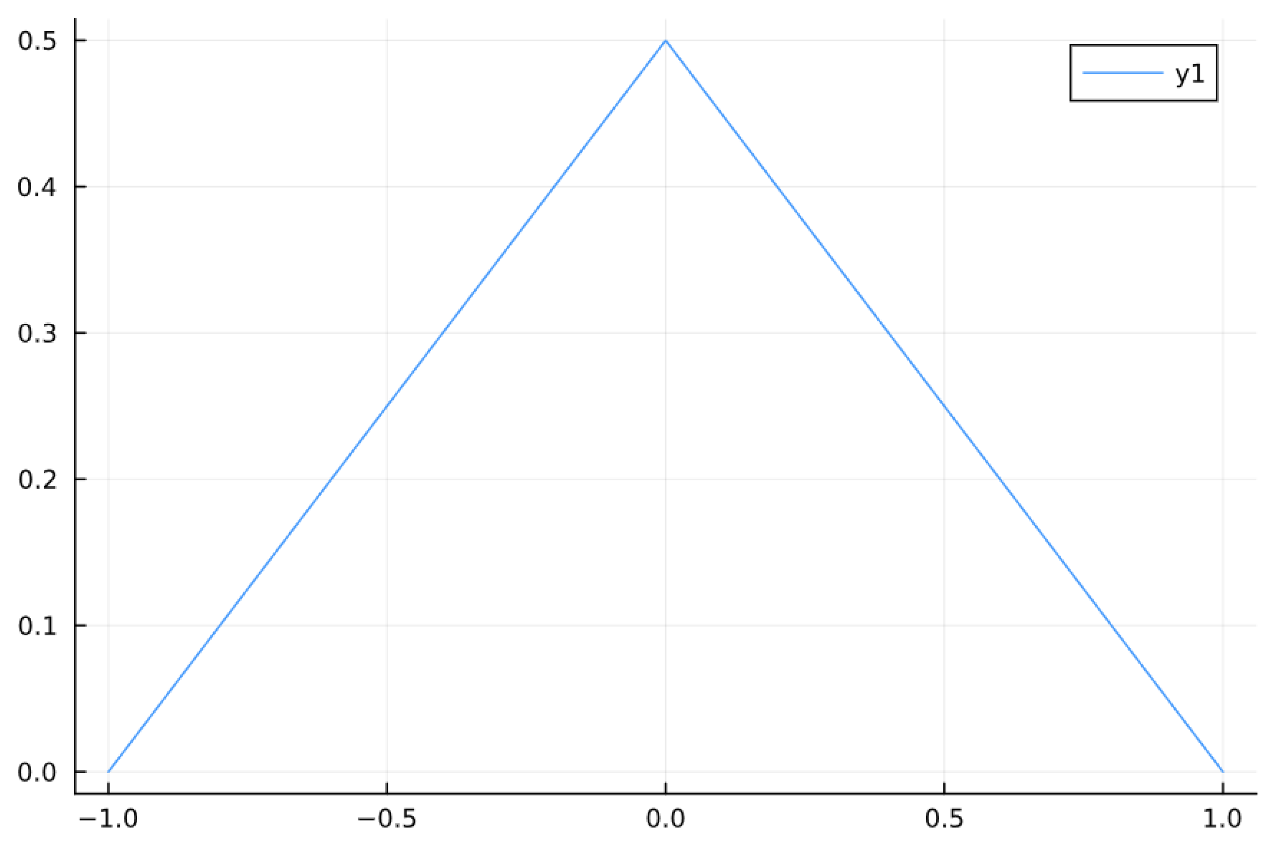
4.1. Screened Poisson in 1D

When it comes to problems with zero Dirichlet boundary conditions, we utilize the basis $\mathbf{Q}$ up to degree i for both the test and trial spaces:

$${\mathbf{Q}}_{0:i}:=\mathbf{Q}\underset{{\mathbf{I}}_{0:i}\in {\mathbb{R}}^{\infty \times D}}{\underbrace{\left[\begin{array}{cccc}{I}_{n-1}& & & \\ & I_n& & \\ & & \ddots & \\ & & & I_n\\ & & & 0_{n\times n}\\ & & & ⋮\end{array}\right]}}=[\tilde{\mathbf{H}}|{\mathbf{W}}_0|\cdots |{\mathbf{W}}_{i-2}].$$

where $D=(i+1)n-1$ is the overall degrees of freedom. Then, to approximate our solution, we express ${\mathbf{u}}_i\in {\mathbb{R}}^D$ such that $u(x)\approx u_i(x):={\mathbf{Q}}_{0:i}(x){\mathbf{u}}_i$. Similarly, we write our test functions as $v_i={\mathbf{Q}}_{0:i}{\mathbf{v}}_i$. The discretisation of our weak form is as follows:

$$\begin{array}{cc}\hfill \langle v_i^{\prime },u_i^{\prime }\rangle +{\omega }^2\langle v_i,u_i\rangle & ={\mathbf{v}}_i^{\top }\langle {({({\mathbf{Q}}_{0:i})}^{\prime })}^{\top },{({\mathbf{Q}}_{0:i})}^{\prime }\rangle {\mathbf{u}}_i+{\omega }^2{\mathbf{v}}_i^{\top }\langle {({\mathbf{Q}}_{0:i})}^{\top },{\mathbf{Q}}_{0:i}\rangle {\mathbf{u}}_i\hfill \\ \hfill & ={\mathbf{v}}_i^{\top }(-\underset{{\Delta }_{Q,i}}{\underbrace{I_{0:i}^{\top }{\Delta }_Q{I}_{0:i}}}+{\omega }^2\underset{M_{Q,i}}{\underbrace{I_{0:i}^{\top }{M}_Q{I}_{0:i}}}){\mathbf{u}}_i.\hfill \end{array}$$

Next, naturally, using the delta function as $f=\delta (x)$, we simplify the right-hand side:

$$\langle v_i,f\rangle ={\mathbf{v}}_i^{\top }{({\mathbf{Q}}_{0:i})}^{\top }f={\mathbf{v}}_i^{\top }{({\mathbf{Q}}_{0:i})}^{\top }\delta ={\mathbf{v}}_i^{\top }\left(\begin{array}{c}\langle {\tilde{\mathbf{H}}}^{\top },\delta \rangle \\ \langle {\mathbf{W}}_0^{\top },\delta \rangle \\ \langle {\mathbf{W}}_1^{\top },\delta \rangle \\ ⋮\\ \langle {\mathbf{W}}_{i-2}^{\top },\delta \rangle \end{array}\right)={\mathbf{v}}_i^{\top }\left(\begin{array}{c}\tilde{\mathbf{H}}{(0)}^{\top }\\ {\mathbf{W}}_0{(0)}^{\top }\\ {\mathbf{W}}_1{(0)}^{\top }\\ ⋮\\ {\mathbf{W}}_{i-2}{(0)}^{\top }\end{array}\right).$$

For the last equality, we use the property of the delta function. Then, imposing this equation for every ${\mathbf{v}}_i\in {\mathbb{R}}^D$ results in a system of $D\times D$ equations:

$$(-{\Delta }_{Q,i}+{\omega }^2{M}_{Q,i}){\mathbf{u}}_i=\left(\begin{array}{c}\tilde{\mathbf{H}}{(0)}^{\top }\\ {\mathbf{W}}_0{(0)}^{\top }\\ {\mathbf{W}}_1{(0)}^{\top }\\ ⋮\\ {\mathbf{W}}_{i-2}{(0)}^{\top }\end{array}\right)$$

where the right-hand side always has many zeros (i.e., it is sparse).

Figure 2 shows the numerical solution of the 1D Poisson equation with a Dirac delta function source located at the origin. The result demonstrates the expected piecewise linear profile, with a maximum at $x=0$ and zero values at the boundaries. This matches the analytical form of the Green’s function in one dimension, given by $u(x)={\displaystyle \frac{1}{2}}(1-|x|)$. The agreement validates the ability of our method to capture the singular structure induced by the delta source.

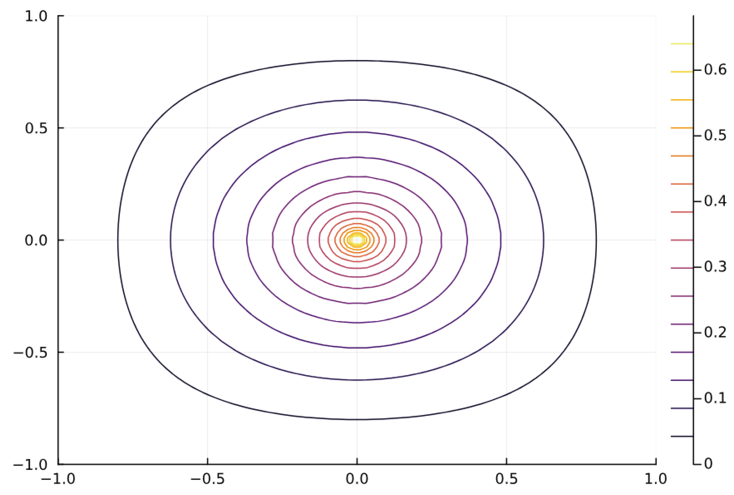
4.2. Screened Poisson in 2D

In 2D, we focus on partitions $x_1<\cdots <x_m$ and $y_1<\cdots <y_n$, truncating degrees i and j, respectively. The basis can then be expressed using the tensor product. We obtain

$$u(x,y)\approx u_{ij}(x,y):={\mathbf{Q}}_{0:i}^{\mathbf{x}}(x)U_{ij}{\mathbf{Q}}_{0:j}^{\mathbf{y}}{(y)}^{\top }$$

where unknown coefficients are signified by $U_{ij}\in {\mathbb{R}}^{M\times N}$. In addition, we can represent $f(x,y)$ as $\delta (x,y)$.

Then, we consider the test function $v_{ij}(x,y)={\mathbf{Q}}_{0:i}^{\mathbf{x}}(x)V_{ij}{\mathbf{Q}}_{0:j}^{\mathbf{y}}(y)$. By inserting u and v into the weak form of the Poisson equation, the left-hand side of our weak formulation becomes as follows:

$$\begin{array}{cc}\hfill & \langle \nabla v,\nabla u\rangle +{\omega }^2\langle v,u\rangle =\langle v_{ij}^x,u_{ij}^x\rangle +\langle v_{ij}^y,u_{ij}^y\rangle +{\omega }^2\langle v,u\rangle \hfill \\ \hfill =& V_{ij}^{\top }\langle {({\mathbf{Q}}_{0:i}^{\mathbf{x}}{(x)}^{\prime })}^{\top },{\mathbf{Q}}_{0:i}^{\mathbf{x}}{(x)}^{\prime }\rangle U_{ij}\langle {\mathbf{Q}}_{0:j}^{\mathbf{y}}{(y)}^{\top },{\mathbf{Q}}_{0:j}^{\mathbf{y}}(y)\rangle +\hfill \\ \hfill & V_{ij}^{\top }\langle {\mathbf{Q}}_{0:i}^{\mathbf{x}}{(x)}^{\top },{\mathbf{Q}}_{0:i}^{\mathbf{x}}(x)\rangle U_{ij}\langle {({\mathbf{Q}}_{0:j}^{\mathbf{y}}{(y)}^{\prime })}^{\top },{\mathbf{Q}}_{0:j}^{\mathbf{y}}{(y)}^{\prime }\rangle +\hfill \\ \hfill & {\omega }^2{V}_{ij}^{\top }\langle {\mathbf{Q}}_{0:i}^{\mathbf{x}}{(x)}^{\top },{\mathbf{Q}}_{0:i}^{\mathbf{x}}(x)\rangle U_{ij}\langle {\mathbf{Q}}_{0:j}^{\mathbf{y}}{(y)}^{\top },{\mathbf{Q}}_{0:j}^{\mathbf{y}}(y)\rangle \hfill \\ \hfill =& V_{ij}^{\top }(-I_{0:i}^{\top }{\Delta }_Q^{\mathbf{x}}{I}_{0:i})U_{ij}(I_{0:j}^{\top }{M}_Q^{\mathbf{y}}{I}_{0:j})+\hfill \\ \hfill & V_{ij}^{\top }(I_{0:i}^{\top }{M}_Q^{\mathbf{x}}{I}_{0:i})U_{ij}(-I_{0:j}^{\top }{\Delta }_Q^{\mathbf{y}}{I}_{0:j})+\hfill \\ \hfill & {\omega }^2{V}_{ij}^{\top }(I_{0:i}^{\top }{M}_Q^{\mathbf{x}}{I}_{0:i})U_{ij}(I_{0:j}^{\top }{M}_Q^{\mathbf{y}}{I}_{0:j})\hfill \\ \hfill =& V_{ij}^{\top }(-{\Delta }_{Q,i}^{\mathbf{x}})U_{ij}{M}_{Q,j}^{\mathbf{y}}+V_{ij}^{\top }{M}_{Q,i}^{\mathbf{x}}{U}_{ij}(-{\Delta }_{Q,j}^{\mathbf{y}})+{\omega }^2{V}_{ij}^{\top }{M}_{Q,i}^{\mathbf{x}}{U}_{ij}{M}_{Q,i}^{\mathbf{y}}\hfill \\ \hfill =& V_{ij}^{\top }\left((-{\Delta }_{Q,i}^{\mathbf{x}})U_{ij}{M}_{Q,j}^{\mathbf{y}}+M_{Q,i}^{\mathbf{x}}{U}_{ij}(-{\Delta }_{Q,j}^{\mathbf{y}})+{\omega }^2{M}_{Q,i}^{\mathbf{x}}{U}_{ij}{M}_{Q,i}^{\mathbf{y}}\right).\hfill \end{array}$$

Then, we use the delta function $f(x,y)=\delta (x,y)$, so we can obtain the right-hand side as follows:

$$\begin{array}{cc}\hfill \langle v,f\rangle & =V_{ij}^{\top }{\mathbf{Q}}_{0:i}^{\mathbf{x}}{(x)}^{\top }f{\mathbf{Q}}_{0:j}^{\mathbf{y}}(y)=V_{ij}^{\top }{\mathbf{Q}}_{0:i}^{\mathbf{x}}{(x)}^{\top }\delta (x,y){\mathbf{Q}}_{0:j}^{\mathbf{y}}(y)=V_{ij}^{\top }{\mathbf{Q}}_{0:i}^{\mathbf{x}}{(x)}^{\top }\delta (x)\delta (y){\mathbf{Q}}_{0:j}^{\mathbf{y}}(y)\hfill \\ \hfill & =V_{ij}^{\top }\left(\begin{array}{c}\langle {\tilde{\mathbf{H}}}^{\top },\delta \rangle \\ \langle {\mathbf{W}}_0^{\top },\delta \rangle \\ \langle {\mathbf{W}}_1^{\top },\delta \rangle \\ ⋮\\ \langle {\mathbf{W}}_{i-2}^{\top },\delta \rangle \end{array}\right)\left(\begin{array}{c}\langle \delta ,\tilde{\mathbf{H}}\rangle ,\langle \delta ,{\mathbf{W}}_0\rangle ,\langle \delta ,{\mathbf{W}}_1\rangle ,\cdots ,\langle \delta ,{\mathbf{W}}_{i-2}\rangle \end{array}\right)\hfill \\ \hfill & =V_{ij}^{\top }\left(\begin{array}{c}\tilde{\mathbf{H}}{(0)}^{\top }\\ {\mathbf{W}}_0{(0)}^{\top }\\ {\mathbf{W}}_1{(0)}^{\top }\\ ⋮\\ {\mathbf{W}}_{i-2}{(0)}^{\top }\end{array}\right)\left(\begin{array}{c}\tilde{\mathbf{H}}(0),{\mathbf{W}}_0(0),{\mathbf{W}}_1(0),\cdots ,{\mathbf{W}}_{i-2}(0)\end{array}\right)\hfill \\ \hfill & =V_{ij}^{\top }\left[\begin{array}{cccc}\tilde{\mathbf{H}}{(0)}^{\top }\tilde{\mathbf{H}}(0)& \tilde{\mathbf{H}}{(0)}^{\top }{\mathbf{W}}_0(0)& \cdots & \tilde{\mathbf{H}}{(0)}^{\top }{\mathbf{W}}_{i-2}(0)\\ {\mathbf{W}}_0{(0)}^{\top }\tilde{\mathbf{H}}(0)& {\mathbf{W}}_0{(0)}^{\top }{\mathbf{W}}_0(0)& \cdots & {\mathbf{W}}_0{(0)}^{\top }{\mathbf{W}}_{i-2}(0)\\ ⋮& ⋮& \ddots & ⋮\\ {\mathbf{W}}_{i-2}{(0)}^{\top }\tilde{\mathbf{H}}(0)& {\mathbf{W}}_{i-2}{(0)}^{\top }{\mathbf{W}}_0(0)& \cdots & {\mathbf{W}}_{i-2}{(0)}^{\top }{\mathbf{W}}_{i-2}(0)\end{array}\right].\hfill \end{array}$$

Therefore, we know

$$\begin{array}{cc}\hfill & (-{\Delta }_{Q,i}^{\mathbf{x}})U_{ij}{M}_{Q,j}^{\mathbf{y}}+M_{Q,i}^{\mathbf{x}}{U}_{ij}(-{\Delta }_{Q,j}^{\mathbf{y}})+{\omega }^2{M}_{Q,i}^{\mathbf{x}}{U}_{ij}{M}_{Q,i}^{\mathbf{y}}\hfill \\ \hfill & =\left[\begin{array}{cccc}\tilde{\mathbf{H}}{(0)}^{\top }\tilde{\mathbf{H}}(0)& \tilde{\mathbf{H}}{(0)}^{\top }{\mathbf{W}}_0(0)& \cdots & \tilde{\mathbf{H}}{(0)}^{\top }{\mathbf{W}}_{i-2}(0)\\ {\mathbf{W}}_0{(0)}^{\top }\tilde{\mathbf{H}}(0)& {\mathbf{W}}_0{(0)}^{\top }{\mathbf{W}}_0(0)& \cdots & {\mathbf{W}}_0{(0)}^{\top }{\mathbf{W}}_{i-2}(0)\\ ⋮& ⋮& \ddots & ⋮\\ {\mathbf{W}}_{i-2}{(0)}^{\top }\tilde{\mathbf{H}}(0)& {\mathbf{W}}_{i-2}{(0)}^{\top }{\mathbf{W}}_0(0)& \cdots & {\mathbf{W}}_{i-2}{(0)}^{\top }{\mathbf{W}}_{i-2}(0)\end{array}\right].\hfill \end{array}$$

Also, we can modify it to Sylvester’s equation:

$$\begin{array}{cc}\hfill & (-{\Delta }_{Q,i}^{\mathbf{x}}+{\displaystyle \frac{{\omega }^2}{2}}{M}_{Q,i}^{\mathbf{x}})U_{ij}{M}_{Q,j}^{\mathbf{y}}+M_{Q,i}^{\mathbf{x}}{U}_{ij}(-{\Delta }_{Q,j}^{\mathbf{y}}+{\displaystyle \frac{{\omega }^2}{2}}{M}_{Q,i}^{\mathbf{y}})\hfill \\ \hfill & =\left[\begin{array}{cccc}\tilde{\mathbf{H}}{(0)}^{\top }\tilde{\mathbf{H}}(0)& \tilde{\mathbf{H}}{(0)}^{\top }{\mathbf{W}}_0(0)& \cdots & \tilde{\mathbf{H}}{(0)}^{\top }{\mathbf{W}}_{i-2}(0)\\ {\mathbf{W}}_0{(0)}^{\top }\tilde{\mathbf{H}}(0)& {\mathbf{W}}_0{(0)}^{\top }{\mathbf{W}}_0(0)& \cdots & {\mathbf{W}}_0{(0)}^{\top }{\mathbf{W}}_{i-2}(0)\\ ⋮& ⋮& \ddots & ⋮\\ {\mathbf{W}}_{i-2}{(0)}^{\top }\tilde{\mathbf{H}}(0)& {\mathbf{W}}_{i-2}{(0)}^{\top }{\mathbf{W}}_0(0)& \cdots & {\mathbf{W}}_{i-2}{(0)}^{\top }{\mathbf{W}}_{i-2}(0)\end{array}\right].\hfill \end{array}$$

Similarly, for the right-hand side of the above equation, it has the sparse structure. Naturally, solving this equation is desirable, despite its structural complexity. For a generalized Sylvester equation,

$$AUB-CUD=E,$$

Using the Alternating Direction Implicit (ADI) method [1,2], including reverse Cholesky factorization, a decomposition of a matrix into the form $A=L^{\top }L$, with L being a lower triangular matrix, is a good way to derive U. The outline of the algorithm is given in Algorithm 1. The shift parameters $p_i$ and $q_i$ used in Algorithm 1 are computed using an explicit analytic formula derived from the theory of elliptic functions and conformal mappings. Specifically, the formulas for $p_i$ and $q_i$ are explicitly given in ([1], Equation (2.4)), based on the Jacobi elliptic function, the complete elliptic integral, and a Möbius transformation that maps reference intervals to the spectral ranges of the system matrices. This choice guarantees near-optimal convergence of the ADI iterations. The convergence rate satisfies the exponential decay bound, as described in ([1], Equation (2.5)).

Algorithm 1 Generalized ADI Solver

Input: Symmetric matrices $A\in {\mathbb{R}}^{m\times m},B\in {\mathbb{R}}^{n\times n},C\in {\mathbb{R}}^{m\times m},D\in {\mathbb{R}}^{n\times n}$, matrix $E\in {\mathbb{R}}^{m\times n}$, and error tolerance $ϵ>0$ Output: Matrix $U\in {\mathbb{R}}^{m\times n}$ such that $AUB-CUD\approx E$ Preprocessing Phase:   1: Compute generalized eigenvalue intervals $\sigma (A,C)$ and $\sigma (B,D)$ via banded symmetric generalized eigen-solvers. Therefore, we can get $\sigma (\tilde{A})$ is in $[a_1,a_2]$ and $\sigma (\tilde{B})$ is in $[b_1,b_2]$ where $a_1,b_1$ are the minimal eigenvalues and $a_2,b_2$ are maximal eigenvalues.   2: Determine the number of ADI iterations: $$K=\lceil \frac{log(16\eta )log(\frac{4}{ϵ})}{{\pi }^2}\rceil ,\eta ={\displaystyle \frac{|b_1-a_1\left|\right|b_2-a_2|}{|b_1-a_2\left|\right|b_2-a_1|}}.$$   3: Calculate the ADI shift parameters ${\left\{p_i\right\}}_{i=1}^K$ and ${\left\{q_i\right\}}_{i=1}^K$, ensuring $p_i>0,q_i<0$.   4: Precompute reverse Cholesky factorizations for $q_{i}A-C$ and $p_{i}D-B$ for each i. Iterative Solution Phase:   1: Initialize $W_0=0$.   2: for $i=1$ to K do   3:     Compute intermediate iterate: $$\begin{array}{cc}\hfill W_{i-{\displaystyle \frac{1}{2}}}& =((A-p_{i}C)W_{i-1}-E){(D-p_{i}B)}^{-1}\hfill \\ \hfill W_i& ={(A-q_{i}C)}^{-1}(W_{i-\frac{1}{2}}(D-q_{i}B)-E)\hfill \end{array}$$   4: end for   5: Output final result: $U=W_K{C}^{-1}$.

By applying this method to our problem, we obtain the coefficient matrix $U_{ij}$, from which the desired solution $u(x,y)$ can be reconstructed. We then present the numerical solution to the Poisson equation with a delta function as the source term. Figure 3 shows a 2D contour plot of the numerical solution. The concentric level lines reflect the radial symmetry of the Green’s function. Figure 4 provides a 3D surface view of the same solution, highlighting the sharp peak at the origin and its smooth radial decay, consistent with the analytical form of the Green’s function, which serves as the impulse response to the Poisson operator.

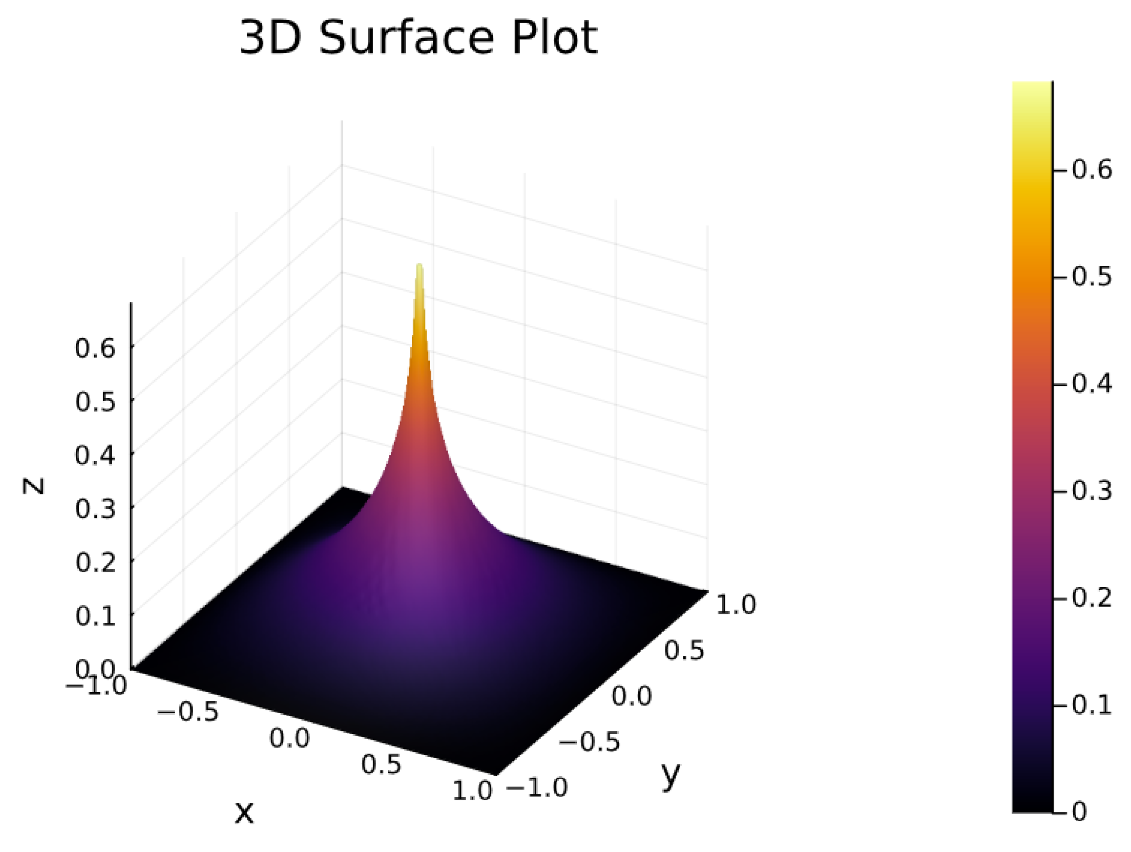
4.3. Screened Poisson in 3D

Consider Poisson’s equation on the cube with homogeneous Dirichlet conditions:

$$-(u_{xx}+u_{yy}+u_{zz})=f,(x,y,z)\in {[-1,1]}^3.$$

(2)

We can discretize the above equation as follows:

$$(D_{xx}+D_{yy}+D_{zz})\mathrm{vec}(X)=\mathrm{vec}(F),$$

(3)

where $X,F\in {\mathbb{C}}^{n\times n\times n}$, $D_{xx}=A\otimes A\otimes I$, $D_{yy}=A\otimes I\otimes A$, and $D_{zz}=I\otimes A\otimes A$ [1]. And, $A=D^{-1}M$ is the pentadiagonal matrix, I is the $n\times n$ identity matrix, ‘⊗’ is the Kronecker product, and $\mathrm{vec}(·)$ is the vectorization operator.

We aim to solve Equation (3) by extending ADI without forming a Kronecker product matrix. But, it is not straightforward to generalize ADI to manage over two terms simultaneously [1,20]. Therefore, we utilize the nested ADI method, as outlined in [4]. This approach entails combining the initial two terms and executing the ADI-like iteration as follows:

$$\begin{array}{cc}\hfill & (D_{zz}-p_{i,1}I)\mathrm{vec}(X_{i+1/2})=\mathrm{vec}(F)-((D_{xx}+D_{yy})-p_{i,1}I)\mathrm{vec}(X_i),\hfill \end{array}$$

(4)

$$\begin{array}{cc}\hfill & \left((D_{xx}+D_{yy})-q_{i,1}I\right)\mathrm{vec}(X_{i+1})=\mathrm{vec}(F)-(D_{zz}-q_{i,1}I)\mathrm{vec}(X_{i+1/2})\hfill \end{array}$$

(5)

for reasonable selection of $p_{i,1}$ and $q_{i,1}$ [1]. Because $D_{xx}$, $D_{yy}$, and $D_{zz}$ are Kronecker products, we can prove that the eigenvalue bounds on $D_{xx}$, $D_{yy}$, and $D_{zz}$ are the same [12,20].

In order to solve Equation (4), nested ADI iteration can be used in matrices $D_{xx}-\frac{q_{i,1}}{2}I$ and $D_{yy}-\frac{q_{i,1}}{2}I$ for [1]

$$\begin{array}{cc}\hfill & F_i-\left(D_{yy}-(q_{i,1}/2)I-p_{j,2}I\right)\mathrm{vec}(Y_j)=\left(D_{xx}-(q_{i,1}/2)I-p_{j,2}I\right)\mathrm{vec}(Y_{i+1/2}),\hfill \end{array}$$

(6)

$$\begin{array}{cc}\hfill & F_i-\left(D_{xx}-(q_{i,1}/2)I-q_{j,2}I\right)\mathrm{vec}(Y_{j+1/2})=\left(D_{yy}-(q_{i,1}/2)I-q_{j,2}I\right)\mathrm{vec}(Y_{j+1})\hfill \end{array}$$

(7)

When it converges, we can see that the solution to Equation (5) is given by $X_{i+1}:=Y_{j+1}$. With the optimal selection of $p_{j,2}$ and $q_{j,2}$, we anticipate that Equations (6) and (7) will converge within $O(logn)$ iterations.

In the final step, we need to solve the three linear systems (4), (6), and (7), each of which involves a shifted Kronecker system. These Kronecker systems are degenerate in one dimension because of the identity matrix. Consequently, we can separate (4), (6), and (7) and solve n independent equations individually [1]. For instance, if we aim to solve (4) for $X_{i+1/2}$, we just need to handle the following:

$$F_i(:,:,t)=A{X}_{i+\frac{1}{2}}(:,:,t)A^{\top }-p_{i,1}{X}_{i+\frac{1}{2}}(:,:,t),1\le t\le n,$$

(8)

where $X(:,:,t)$ signifies the tth slice of X along third dimension and $F_i=\mathrm{vec}(F)-(D_{xx}+D_{yy}-p_{i,1}I)\mathrm{vec}(X_i)$. For solving Equation (8), an additional nested ADI iteration can be executed. Next, we can rewrite (8) as follows:

$$A^{-1}{F}_i(:,:,t)=p_{i,1}{A}^{-1}{X}_{i+\frac{1}{2}}(:,:,t)-X_{i+\frac{1}{2}}(:,:,t)A^{\top }.$$

The iteration for each value of t is given as follows:

$$\begin{array}{cc}\hfill A^{-1}{F}_i(:,:,t)-(p_{i,1}{A}^{-1}-p_{l,3}I)Z_l& =Z_{l+\frac{1}{2}}(A^{\top }-p_{l,3}I),\hfill \end{array}$$

(9)

$$\begin{array}{cc}\hfill A{F}_i(:,:,t)-A{Z}_{l+\frac{1}{2}}(A^{\top }-p_{l,3}I)& =(p_{i,1}I-q_{l,3}A)Z_{l+1}.\hfill \end{array}$$

(10)

Once the iteration converges, the solution to (4) for each k is obtained as $X_{i+1/2}(:,:,k):=Z_{l+1}$. It is important to note that (7) has been multiplied by A to allow for faster solving of (6) and (7).

In this paper, again, we use delta function $f(x,y,z)=\delta (x,y,z)$. From previous discussion, we know the specific F, which is the sparse tensor for the right-hand side using the property of delta function.

Figure 5 illustrates the numerical solution to the Poisson equation with a delta function source in three dimensions. To visualize the behavior of the solution, we plot cross-sectional slices of the scalar field on the coordinate planes $xy$, $yz$, and $xz$. The result shows a bright central peak at the origin, consistent with the singular nature of the Dirac delta source, and smooth radial decay outward. The star-like shape arises from the intersection of three orthogonal heatmaps, each corresponding to a fixed coordinate plane. It is important to note, however, that while this method is recognized for its optimal complexity in spectral methods for solving Equation (2), it is not considered a practical algorithm. The reason is that the inner iterations of the Alternating Direction Implicit (ADI) method must be computed with machine precision to ensure convergence of the outer iterations [1].

5. Computational Cost Analysis

The computational cost of the proposed method is primarily driven by two factors: the sparse system matrix construction and the iterative ADI solution procedure. Below, we discuss the computational complexity of each step.

5.1. Sparse Matrix Construction

The system matrix in our method is sparse, resulting from the use of Legendre polynomials as basis functions in the FEM framework. These polynomials are orthogonal, leading to a system matrix with a Banded-Block-Banded-Arrowhead ($B^3$-Arrowhead) sparsity pattern. The sparsity structure significantly reduces the computational cost, as only a limited number of non-zero entries are present in the matrix, particularly in higher dimensions.

In the 1D case, the system matrix consists of the mass matrix and the weak Laplacian matrix. The mass matrix arises from the inner products of the operator derived from basis functions, while the weak Laplacian matrix corresponds to the inner products of derivative of the operator. The construction of the mass and weak Laplacian matrices involves matrix multiplication, which requires $\mathcal{O}(N)$ operations, where N is the number of degrees of freedom in one direction. When extending to 2D and 3D, the complexity increases to $\mathcal{O}(N^2)$ and $\mathcal{O}(N^3)$, respectively, because of the the increased number of degrees of freedom. Despite the growth, the banded-block-banded structure of the matrices ensures that they remain sparse, reducing both memory usage and computational time.

5.2. ADI Iterative Algorithm

The solution of the system is performed using the Alternating Direction Implicit (ADI) algorithm, which has been shown to achieve near-optimal computational complexity.

For the preprocessing phase, which includes constructing and factorizing matrices, the computational cost is $\mathcal{O}(N^2+KN)$, where K is the number of iterations. The $\mathcal{O}(N^2)$ term comes from the matrix construction (especially for 2D), while the $\mathcal{O}(KN)$ term accounts for the cost of computing reverse Cholesky factorization. When considering the iterative solution phase, the computational cost for obtaining a solution is $\mathcal{O}(K{N}^2)$ in 2D and $\mathcal{O}(K{N}^3)$ in 3D, as each ADI step involves performing multiplication and inversion. The number of iterations K remains small due to the choice of shift parameters, keeping the method efficient in practice.

5.3. Scalability and Parallelization

The method is highly parallelizable due to the fact that the ADI iterations are independent in each direction. This parallelism enables the method to scale efficiently for large grids, with each iteration being handled by multiple processors or computational nodes in parallel. Thus, the overall performance can be further improved for large-scale 2D and 3D problems, making the method well-suited for high-performance computing environments.

6. Conclusions

This paper presents a numerical framework for solving the screened Poisson equation with Dirac delta forcing using sparse finite element methods. By adopting integrated Legendre functions as basis functions, we derive structured variational formulations that lead to sparse system matrices, specifically exhibiting a Banded-Block-Banded-Arrowhead ($B^3$-Arrowhead) structure.

We develop and analyze discretizations that effectively resolve the singular behavior induced by the delta function. In higher dimensions, we employ the Alternating Direction Implicit (ADI) method with reverse Cholesky factorization to preserve sparsity and ensure computational efficiency.

Numerical results demonstrate that the solution exhibits a peak at the origin and decays symmetrically outward, consistent with the characteristics of Green’s functions in classical potential theory. These results further indicate that combining sparse FEM structures with integrated Legendre functions yields a robust and stable framework for solving PDEs with singular forcing—an area not systematically addressed in previous work.

The proposed approach offers a general and effective tool for handling impulsive source terms in elliptic PDEs, with promising applications in physics, engineering, and computational mathematics.

Future work may explore extensions to more complex domains, such as circular or spherical geometries, as well as alternative forcing terms beyond the delta function. Additionally, extending the framework to accommodate mixed boundary conditions (e.g., combinations of Dirichlet and Neumann boundaries) enhances its applicability in practical scenarios and introduces new challenges in preserving the sparse structure and solver efficiency.

References

1. Fortunato, D.; Townsend, A. Fast Poisson solvers for spectral methods. IMA J. Numer. Anal. 2020, 40, 1994–2018. [Google Scholar] [CrossRef]
2. Knook, K.; Olver, S.; Papadopoulos, I. Quasi-optimal complexity hp-FEM for Poisson on a rectangle. arXiv 2024, arXiv:2402.11299. [Google Scholar]
3. Babuška, I.; Craig, A.; Mandel, J.; Pitkäranta, J. Efficient preconditioning for the p-version finite element method in two dimensions. SIAM J. Numer. Anal. 1991, 28, 624–661. [Google Scholar] [CrossRef]
4. Wachspress, E.L. Three-variable alternating-direction-implicit iteration. Comput. Math. Appl. 1994, 27, 1–7. [Google Scholar] [CrossRef]
5. Schwab, C. p-and hp-Finite Element Methods: Theory and Applications in Solid and Fluid Mechanics; Clarendon Press: Oxford, UK, 1998. [Google Scholar]
6. Szabó, B.; Babuška, I. Introduction to Finite Element Analysis: Formulation, Verification and Validation; John Wiley & Sons: Hoboken, NJ, USA, 2011. [Google Scholar]
7. Beuchler, S.; Schoeberl, J. New shape functions for triangular p-FEM using integrated Jacobi polynomials. Numer. Math. 2006, 103, 339–366. [Google Scholar] [CrossRef]
8. Babuška, I.; Suri, M. The p and h-p versions of the finite element method, basic principles and properties. SIAM Rev. 1994, 36, 578–632. [Google Scholar] [CrossRef]
9. Beuchler, S.; Pechstein, C.; Wachsmuth, D. Boundary concentrated finite elements for optimal boundary control problems of elliptic PDEs. Comput. Optim. Appl. 2012, 51, 883–908. [Google Scholar] [CrossRef]
10. Beuchler, S.; Pillwein, V. Sparse shape functions for tetrahedral p-FEM using integrated Jacobi polynomials. Computing 2007, 80, 345–375. [Google Scholar] [CrossRef]
11. Dubiner, M. Spectral methods on triangles and other domains. J. Sci. Comput. 1991, 6, 345–390. [Google Scholar] [CrossRef]
12. Houston, P.; Schwab, C.; Süli, E. Discontinuous hp-finite element methods for advection-diffusion-reaction problems. SIAM J. Numer. Anal. 2002, 39, 2133–2163. [Google Scholar] [CrossRef]
13. Jia, L.; Li, H.; Zhang, Z. Sparse spectral-Galerkin method on an arbitrary tetrahedron using generalized Koornwinder polynomials. J. Sci. Comput. 2022, 91, 22. [Google Scholar] [CrossRef]
14. Karniadakis, G.; Sherwin, S.J. Spectral/hp Element Methods for Computational Fluid Dynamics; Oxford University Press: Oxford, MS, USA, 2005. [Google Scholar]
15. Pavarino, L.F. Additive Schwarz methods for the p-version finite element method. Numer. Math. 1993, 66, 493–515. [Google Scholar] [CrossRef]
16. Snowball, B.; Olver, S. Sparse spectral and-finite element methods for partial differential equations on disk slices and trapeziums. Stud. Appl. Math. 2020, 145, 3–35. [Google Scholar] [CrossRef]
17. Averbuch, A.; Israeli, M.; Vozovoi, L. A fast Poisson solver of arbitrary order accuracy in rectangular regions. SIAM J. Sci. Comput. 1998, 19, 933–952. [Google Scholar] [CrossRef]
18. Wikipedia Contributors. 2024. Available online: https://en.wikipedia.org/wiki/Diracdeltafunction (accessed on 10 January 2025).
19. Olver, S.; Slevinsky, R.M.; Townsend, A. Fast algorithms using orthogonal polynomials. Acta Numer. 2020, 29, 573–699. [Google Scholar] [CrossRef]
20. Olver, S.; Townsend, A. A fast and well-conditioned spectral method. SIAM Rev. 2013, 55, 462–489. [Google Scholar] [CrossRef]
Figure 1. Visual image of Dirac delta function.
Mathematics 13 01360 g001
Figure 2. Numerical solution to the 1D Poisson equation with a delta function source, Δ u ( x ) = δ ( x ) , subject to homogeneous Dirichlet boundary conditions on [ 1 , 1 ] . The solution exhibits a sharp peak at x = 0 and linear decay to the boundaries, consistent with the analytical Green’s function.
Mathematics 13 01360 g002
Figure 3. 2D contour plot of the solution to Δ u ( x , y ) = δ ( x , y ) . The solution exhibits radial symmetry and a sharp peak at the origin, corresponding to the Dirac delta source.
Mathematics 13 01360 g003
Figure 4. 3D surface plot of the solution to Δ u ( x , y ) = δ ( x , y ) . The plot shows the peaked behavior around the origin and symmetric decay outward, consistent with the structure of Green’s function.
Mathematics 13 01360 g004
Figure 5. Cross-sectional heatmap views of the numerical solution to the 3D Poisson equation with a Dirac delta source, Δ u ( x , y , z ) = δ ( x , y , z ) . The solution exhibits radial symmetry and a sharp peak at the origin, decaying smoothly in all directions. The figure shows slices of the solution on the x y -, x z -, and y z -planes.
Mathematics 13 01360 g005
Disclaimer/Publisher’s Note: The statements, opinions and data contained in all publications are solely those of the individual author(s) and contributor(s) and not of MDPI and/or the editor(s). MDPI and/or the editor(s) disclaim responsibility for any injury to people or property resulting from any ideas, methods, instructions or products referred to in the content.