Abstract
Attitude preference plays an important role in multigranulation data mining and decision-making. That is, different attitude preferences lead to different results. At present, both optimistic and pessimistic multigranulation rough sets have been studied independently and thoroughly. But, sometimes, a decision-maker’s attitude may vary, which may shift either from an optimistic to pessimistic view of decision-making or from a pessimistic to optimistic view of decision-making. In this paper, we propose a novel multigranulation rough set model, which synthesizes optimistic and pessimistic attitude preferences. Specifically, we put forward methods to evaluate the attitude preferences in four types of decision systems. Two main issues are addressed with regard to attitude preference dependency. The first is concerned with the common attitude preference, while the other relates to the sequence-dependent attitude preference. Finally, we present three types of multigranulation rough set models from the perspective of the different connection methods between optimistic and pessimistic attitude preferences.
MSC:
68T37
1. Introduction
Rough set theory was originally proposed by Pawlak [1] in 1982 as a new mathematical tool to measure uncertain concepts. As is well known, in the standard version, the notion of a rough set was considered to be a formal approximation of a crisp set with a pair of sets that were respectively called the lower and upper approximations of the crisp set. Since then, this promising research tool has attracted many researchers, and the development of rough sets, extensions, generalizations, and applications has continued to evolve. Now, it has become an extremely useful approach in data mining, knowledge discovery, and machine learning as an important component of hybrid solutions [2,3].
In the standard version of rough sets, equivalence relations were used as the building blocks to characterize more complicated concepts. However, this may not be valid in more complicated information systems. In order to solve this problem, some important studies have focused on extensions and generalizations of the standard version of a rough set. As a result, the developed rough set theory was used in a broader area than ever before and no longer confined to the traditional information systems [4,5,6,7,8]. Then, some novel rule acquisition methods in different kinds of decision systems [9,10] were explored as their by-products.
From the perspective of granular computing, named by Zadeh [11] and recently developed by many experts [12,13,14], the above kinds of rough set models in fact discussed the issue of characterizing a given set by only one granulation. But, sometimes, we have to solve a problem involving multiple granulations in many real applications. For instance, multiple granulations were used for describing a multi-scale dataset [15], and how to select an optimal granulation was investigated for extracting the best rules. Multi-source information fusion approaches induced by pessimistic multigranulation rough sets and optimistic multigranulation rough sets [16,17] were studied and shown to be better than the classical rough sets in terms of decision-making, which were further generalized to cater to datasets equipped with incomplete, neighborhood, covering, or fuzzy attributes [18,19,20,21]. Moreover, the pessimistic and optimistic multigranulation rough sets immediately led to the development of new types of decision rules that can be measured by support and certainty factors [16,17]. In recent years, some new results have been obtained. For example, Tan et al. [22] applied evidence theory to the numerical characterization of multigranulation rough sets in incomplete information systems. Qian et al. proposed local multigranulation decision-theoretic rough sets [23] as a semi-unsupervised learning method. She et al. developed a multiple-valued logic method for a multigranulation rough set model [24].
Note that the theory of three-way decisions proposed by Yao [3] and further investigated by other researchers [25,26,27,28,29] can be unified with the description framework of multigranulation rough sets and the superiority of concept lattices for allowing more applications. For example, Qian et al. [30] established a new decision-theoretic rough set from the perspective of multigranulation rough sets. Sun et al. [31] discussed three-way group decision-making over two universes using multigranulation fuzzy decision-theoretic rough sets.
In the aforementioned studies, learning cost was not deliberately considered. However, cost-sensitive learning problems frequently appear in many real applications, such as medical treatment, machine fault diagnosis, equipment-automated testing, buffer management, internet-based distributed systems, and others [32]. Note that, in these fields, the main cost may be different, and it includes money, skilled labor, time, memory, bandwidth, and the ways we should pay. In the past decade, cost-sensitive learning systems with different types of costs were intensively studied, including learning cost [33,34], test cost [35], and both of them simultaneously [36,37]. In the meanwhile, cost-sensitive decision systems focused on decision-making problems were also investigated in [35,38,39].
Facing various kinds of costs, different people may have different considerations, which lead to different attitude preferences. For example, rich people may choose to save labor force or time cost, while ordinary ones may take money as their first concern. One may be optimistic on some costs but be pessimistic on others. In other words, the state of optimist or pessimist may not be stable for complicated problems, and it depends on the resources one has and the situations one faces.
Motivated by the above problem, the current study is concerned with the settlement of the unstable attitude preference under a multi-source information fusion environment. More specifically, we provide a method of evaluating attitude preference. Then, F-multigranulation rough sets are proposed to synthesize optimistic and pessimistic attitude preferences, which contain three categories: -multigranulation rough sets, -multigranulation rough sets, and -multigranulation rough sets. Moreover, the relationships among the three types of multigranulation rough sets are analyzed.
The rest of this paper is organized as follows. Section 2 reviews some basic notions related to the classical, pessimistic, and optimistic multigranulation rough sets and concept lattice and introduces their induced rules accordingly. Section 3 develops some useful methods to evaluate the attitude preferences in four kinds of decision systems, where two main issues are addressed with regard to attitude preference dependency. The first is concerned with the common attitude preference, while the other relates to the sequence-dependent attitude preference. Section 4 puts forward three types of multigranulation rough set models based on the different connection methods between optimistic and pessimistic attitude preferences. Section 5 concludes the paper with a brief summary and an outlook for our forthcoming study.
2. Preliminaries
In this section, some basic notions are recalled to make our paper self-contained.
2.1. Classical Rough Set Model
In rough set theory, it starts with an information system and can be defined formally as follows.
Definition 1
([1]). An information system is a tuple , where U is a universe of discourse and is a non-empty finite attribute set.
In fact, for any attribute a of , is denoted to map an object of U to exactly one value. Note that the value category will divide the information systems into different classes (e.g., classical, fuzzy, or interval-valued information systems). In this paper, we only consider the classical information systems.
Moreover, when making decisions, we need to extend an information system to a decision system . In other words, compared to an information system, a decision system contains a decision attribute set D additionally.
Moreover, with each , we can define an equivalence relation
which can be described as from a semantic view, where . Note that all induced by the equivalence relation form a partition of the universe of discourse U. Furthermore, for a target set , we call the classical rough set of X with respect to , where
2.2. Multigranulation Rough Sets and the Corresponding Rules
It can be seen from Section 2.1 that, in the standard version, rough sets are defined based on a single equivalence relation. Similarly, by extending a single equivalence relation to a family of them, multigranulation rough sets can be developed.
Definition 2
([17]). Let S be an information system and . Then, we call the ordered pair pessimistic multigranulation rough set of X with respect to the attribute sets , where
Let be a decision system and . Then, generates an “AND” decision rule as follows:
Definition 3
([16]). Let S be an information system and . Then, we call the ordered pair optimistic multigranulation rough set of X with respect to the attribute sets , where
Let be a decision system and . Then, leads to an “OR” decision rule as follows:
3. A Method to Evaluate Attitude Preferences
This section puts forward a method to evaluate attitude preferences. Let be an information system. On one hand, we define an attribute subset preference function as
where R is the set of real numbers. On the other hand, we define an attribute subset preference mapping as
where O and P denote optimistic and pessimistic attitudes, respectively. Furthermore, the attribute subset preference function and mapping are related as follows: for any ,
Note that the detailed value of will be set under certain types of information systems to be discussed below.
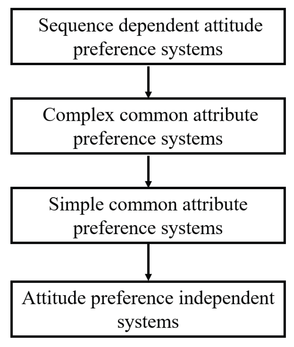
In what follows, we will discuss four types of information systems with regard to attitude preference dependency, and the connections between the four types of information systems are shown in Figure 1, where the system above is a special case of the system below; in other words, the system above can degenerate into the system below.
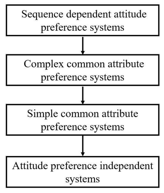
Figure 1.
The connections between four types of information systems.
To aid reader orientation, we provide a glossary of key notations before proceeding.
: attitude-preference-independent system.
: simple common attribute preference system.
: complex common attribute preference system.
: sequence-dependent attitude preference system.
: multigranulation lower approximations of X.
: multigranulation upper approximations of X.
: multigranulation lower approximations of X.
: multigranulation upper approximations of X.
: multigranulation lower approximations of X.
: multigranulation upper approximations of X.
3.1. Attitude-Preference-Independent Systems
In many real applications, attitude preferences are independent. In other words, after taking test-cost attitudes into consideration, we can define a type of new information system.
Definition 4.
An attitude-preference-independent system is the 3-tuple , where is an attribute preference degree function.
An attribute preference degree function can easily be represented by a vector . Note that, in accordance with Equation (7),
(i) we take optimistic attitude on an attribute a if ;
(ii) otherwise, we take pessimistic attitude on an attribute a if .
In this paper, for any with at least two attitudes, we use to denote the attitude preference degree of A when all of its attributes have been taken into consideration simultaneously. It is apparent that, for any , we have .
In an attitude-preference-independent system , we have
which indicates the independence property of attitude preference.
Example 1.

Let be an attitude-preference-independent system, where the attribute preference degree function v is shown in Table 1 and . For , we have and . That is, we will take an optimistic attitude for A.
Table 1.
An attribute preference degree function v.
3.2. Simple Common Attribute Preference Systems
In some real applications, a group of attributes share a simple degree of preference for common attributes. For example, a blood sample collected from a patient can be used to test a set of indicators in diagnosis. In many cases, some indicators are closely related. As a consequence, their preference degrees are also related, and they may share a common attribute preference degree for various types of blood tests [32].
Definition 5.
A simple common attribute preference system is the 5-tuple , where is the simple group-membership function, and is the group common attribute preference degree function. The kth group () is constituted by , and attributes in the group share a common test-cost attitude .
Let and . Then, we have
Similar to the case in Section 3.1,
(i) if the kth group represents optimistic attitudes, then ;
(ii) otherwise, if the kth group represents pessimistic attitudes, then .
Example 2.
Let be a simple common attribute preference system, where the attribute preference degree function v, the group-membership function g, and the group common attribute preference degree function are shown in Table 1, Table 2 and Table 3, respectively. For , by a recursive method, we have
Table 2.
A group-membership function.
Table 3.
A group common attribute preference degree function.
Then, based on Equation (8), it follows that , which means that we will be pessimistic when facing the factors labor, time, memory, and bandwidth simultaneously.
3.3. Complex Common Attribute Preference Systems
In a simple common attribute preference system, an attribute is assumed to be exactly included in one group. But, on some occasions, an attribute may belong to more than one group. The following model caters to such a situation.
Definition 6.
A complex common attribute preference system is the 5-tuple , where is the complex group-membership function. The kth group () is constituted by , and attributes in the group share a common attribute preference degree.
Let and . Then, we have
where the function is defined as
It is interesting that Equation (10) will be degenerated into Equation (9) when the attribute a belongs to one group only. For example, suppose that the attribute a belongs to the group t () only. Then,
and, in this case, Equation (10) will be degenerated into
Moreover, for better understanding of the complex group-membership function , it can be represented by a matrix
where the row i represents the ith group , the column j represents the jth attribute , and the value in the cross of the ith row and jth column is defined as
Example 3.
Let be a complex common attribute preference system, where the attribute preference degree function v, the complex group-membership function , and the group common attribute preference degree function are shown in Table 1, Table 4 and Table 3, respectively. According to the above discussion, Table 4 can be equivalently transformed into Table 5. That is, .
Table 4.
A complex group-membership function.
Table 5.
A complex group-membership function.
Let . Then, we have
Furthermore, we have , which means that we will take an optimistic attitude when facing all the factors, money, labor, time, memory, and bandwidth, simultaneously.
3.4. Sequence-Dependent Attitude Preference Systems
In some real applications, if we take execution order into consideration, the outcome may be different. For example, one possible way is to take money as our first priority. Then, we will save labor and time simultaneously. On the other hand, if we choose to complete the work by ourselves, then we can save some labor force and money, but the cost of time cannot be reduced.
Definition 7.
A sequence-dependent attitude preference system is the 4-tuple , where is the conditional attitude preference degree function. That is, for and , is the attitude preference degree of after the attributes of have been considered.
As mentioned at the beginning of Section 3, is the attitude preference degree of A when all the attributes of A have been taken into consideration simultaneously.
Note that the simplest way of representing the function is to use a -dimensional vector. Moreover, the simplest representation of the function is to use a matrix as follows:
Let denote the attitude preference degree of a sequence , . Then,
Moreover, by using the above formula recursively, we can compute the attitude preference degree of a sequence of , , ⋯, . That is,
Apparently, there may be different execution orders for a sequence of , , ⋯, . For our purpose, we can choose such an execution order for a given sequence that can bring the highest attitude preference degree.
Definition 8
([40]). For and , let . If
we hold that and are sequence-independent.
Proposition 1.
For and , let . If and are sequence-independent, then
Proof.
Since and are sequence-independent, it follows . On the other hand, we have . To sum up, we obtain .
Moreover, can be proved in a similar manner. □
It should be pointed out that simultaneously is most effective while separately is least effective. That is,
It is evident that, if and are attitude-independent (e.g., as in Section 3.1), then and are sequence-independent.
Example 4.
Consider three symptoms caused by flu, which are fever, headache, and cough. For simplicity, we use f, h, and c to represent fever, headache, and cough, respectively.
First, as fever will cause headache and soon follows cough, fever is our first concern. Then, it is reasonable that we will take pessimistic attitude on fever and take optimistic attitude on headache and cough.
Second, as these three symptoms are correlated with each other, then the degree of is less than that of and the degree of is less than that of , where .
Finally, by rating the importance of these three symptoms as well as their combinations, we can assign the values of the preference degree functions v and .
As another example, without giving the details, we provide one reasonable assignment of functions v and as follows:
Then, we have
and follows. In other words, we will take an optimistic attitude when facing all the symptoms, fever, headache, and cough, simultaneously.
4. Multigranulation Rough Sets: A Useful Way to Synthesize Optimistic and Pessimistic Attitudes
In this section, according to the different ways of synthesizing optimistic and pessimistic attitudes, we put forward multigranulation rough sets, multigranulation rough sets, and multigranulation rough sets. Moreover, we uniformly call these three kinds of multigranulation rough sets multigranulation rough sets. Furthermore, in order to distinguish multigranulation rough sets from the classical ones, we call the classical optimistic and pessimistic multigranulation rough sets multigranulation rough sets.
In what follows, for the sake of clarity, any subset of is assumed to take a certain attitude preference. That is, can be computed by the four methods introduced in Section 3.
4.1. Multigranulation Rough Sets and Their Induced Rules
Before embarking on establishing the multigranulation rough set model, we need to emphasize that the information systems to be discussed below are among the four attitude preference systems introduced in Section 3. If one does not want to point out which kind of attitude preference system he/she discusses, then it can simply be called an attitude preference system.
Definition 9.
Let S be an attitude preference information system, , be an index set, and be the attitude preference of . Then, the multigranulation lower and upper approximations of X are, respectively, defined as
where ∨ and ∧ are the logical disjunction and conjunction operators, respectively, and the symbol means that an optimistic attitude is adopted in synthesizing optimistic and pessimistic attitudes.
The pair is referred to as the multigranulation rough set of X with respect to the attribute sets .
According to this definition, for any , it induces the following “AND–OR” decision rule from an attitude preference decision system:
and at least one of and is true, where .
Moreover, the support factor of the rule is defined as
where and .
Moreover, the certainty factor of this rule is defined as
where and .
Example 5.
Consider descriptions of six persons in Table 6 who suffer (or do not suffer) from flu. For each person, four indicators that may cause flu are considered: sneeze, temperature, headache, and cough. For example, person does not cough, has a normal temperature, and does not suffer from headache and cough, so it can be seen that is not a flu-infected patient.
Table 6.
A flu dataset.
Let , (: sneeze, : temperature, : headache, : cough, and d: flu). According to the empirical knowledge of experts, sneezing is a characterization of bacteria infection that leads to a change in body temperature. Soon come headache and cough. In this circumstance, for the treatment of flu, the importance of sneezing will be ranked first, followed by temperature. So, it is reasonable that
Take , , , , and then the attitude we take in each attitude can be shown in Table 7. Concretely, the attitude on and is positive and the attitude on and is negative.
Table 7.
An attitude preference vector.
We can compute the partitions of the universe of discourse:
We have
Then, we obtain the following “AND–OR” decision rules from the attitude preference decision system S in Table 6 using multigranulation rough sets:
Moreover, we have
Likewise, we can obtain
Proposition 2.
Let S be an attitude preference information system, , and be an index set. Then, the following properties hold:
(i) ,
(ii) .
Proof.
At first, we prove . For any and , we have due to . Therefore, it follows that
According to Definition 9, we conclude .
Secondly, we prove . For any and , we have . Therefore, it follows that
According to Definition 9, we obtain .
Moreover, we prove . According to Definition 9, we have
Finally, we prove . According to Definition 9, we have
To sum up, we have completed the proof of Proposition 2. □
By Proposition 2, we find that the lower and upper approximations of two special sets (empty set and universe of discourse) are the lower and upper approximations of themselves.
Proposition 3.
Let S be an attitude preference information system, , and be an index set. Then, for any , and , the following properties hold:
(i) ,
(ii) .
Proof .
(i) Since , we have
Hence, we obtain .
(ii) Based on the result of (i), we have
To sum up, we have completed the proof of Proposition 3. □
By Proposition 3, we can observe that the lower and upper approximations of a target concept become larger as the size of the target concept increases. Thus, if an inclusion relationship exists between the two sets, their lower and upper approximations also satisfy the inclusion relationship.
4.2. Multigranulation Rough Sets and Their Induced Rules
Definition 10.
Let S be an attitude preference information system, , be an index set, and be the attitude preference of . Then, the multigranulation lower and upper approximations of a subset X of U are, respectively, defined as
where the symbol represents that only pessimistic attitude is considered when we synthesize optimistic and pessimistic attitudes.
The pair is referred to as the multigranulation rough set of X with respect to the attribute sets .
According to this definition, for any , it induces the following “AND” decision rule from an attitude preference decision system:
Moreover, the support factor of is defined as
and the certainty factor of this rule is defined as
Example 6.
Continued from Example 5. We have
Then, we obtain the following “AND” decision rules:
Moreover, we compute
Proposition 4.
Let S be an attitude preference information system, , and be an index set. Then, the following properties hold:
(i) ,
(ii) .
Proof.
This proposition can be proved in an analogous manner to that of Proposition 2. □
By Proposition 4, we find that the lower and upper approximations of two special sets (empty set and universe of discourse) are the lower and upper approximations of themselves.
Proposition 5.
Let S be an attitude preference information system, , and be an index set. Then, for any and , the following properties hold:
(i) ,
(ii) .
Proof.
This proposition can be proved in an analogous manner to that of Proposition 3. □
By Proposition 5, we can observe that the lower and upper approximations of a target concept become larger as the size of the target concept increases. Thus, if an inclusion relationship exists between two sets, their lower and upper approximations also satisfy the inclusion relationship.
Proposition 6.
Let S be an attitude preference information system, , and be an index set. Then, for any , the following properties hold:
(i) ,
(ii) .
Proof .
(i) Note that
Thus, we obtain .
(ii) We have and . Then, based on the result of (i), we have , which leads to . That is, . □
In other words, Proposition 6 shows the relationships between the approximations of multigranulation rough sets and multigranulation rough sets.
4.3. Multigranulation Rough Sets and Their Induced Rules
Definition 11.
Let S be an attitude preference information system, , be an index set, and be the attitude preference of . Then, the multigranulation lower and upper approximations of a subset X of U are, respectively, defined as
where the symbol represents that pessimistic attitude is held when we synthesize optimistic and pessimistic attitudes.
The pair is referred to as the multigranulation rough set of X with respect to the attribute sets .
According to this definition, for any , it induces the following “AND–OR” decision rule from a attitude preference decision system:
Obviously, at least one decision rule is true, where .
Moreover, the support factor of is defined as
where and .
Moreover, the certainty factor of this rule is defined as
where and .
Example 7.
Continued from Example 5. We have
Then, we obtain the following “AND–OR” decision rules from the attitude preference decision system S in Table 6 using multigranulation rough sets:
Moreover, we calculate
Likewise, we compute
Proposition 7.
Let S be an attitude preference information system, , and be an index set. Then, the following properties hold:
(i) ,
(ii) .
Proof.
This proposition can be proved in an analogous manner to that of Proposition 2. □
By Proposition 7, we find that the lower and upper approximations of two special sets (empty set and universe of discourse) are the lower and upper approximations of themselves.
Proposition 8.
Let S be an attitude preference information system, , and be an index set. Then, for any and , the following properties hold:
(i) ,
(ii) .
Proof.
This proposition can be proved in an analogous manner to that of Proposition 3. □
By Proposition 8, we can observe that the lower and upper approximations of a target concept become larger as the size of the target concept increases. Thus, if an inclusion relationship exists between two sets, their lower and upper approximations also satisfy the inclusion relationship.
Proposition 9.
Let S be an attitude preference information system, , and be an index set. Then, for any , the following properties hold:
(i),
(ii).
Proof.
This proposition can be proved in an analogous manner to that of Proposition 6. □
That is to say, Proposition 10 shows the relationships between the approximations of multigranulation rough sets and multigranulation rough sets.
4.4. A Comparative Study of Multigranulation Rough Sets and Multigranulation Rough Sets
To facilitate the subsequent discussion, we denote optimistic and pessimistic multigranulation rough sets (see Qian et al. [16,17] for details) by multigranulation rough sets and multigranulation rough sets, respectively.
- (i)
- multigranulation rough sets will be degenerated into multigranulation rough sets in some cases.
Let S be an attitude preference information system, , be an index set, and be the attitude preference of . If, for any , we have , then multigranulation rough sets can be viewed as multigranulation rough sets. Otherwise, if, for any , we have , then multigranulation rough sets can be viewed as multigranulation rough sets.
Proposition 10.
Let S be an attitude preference information system, , and be an index set. Then, for any , the following properties hold:
(1) ,
(2) .
Proof .
(1) At first, we prove . Note that
Thus, we obtain .
Secondly, we prove . Note that
Thus, we have .
Combining the above results with (i) of Propositions 6 and 9, we complete the proof of the first item.
(2) We prove . Then, we have and . Since based on the conclusion obtained in (i), it follows that . That is, .
Secondly, we prove . Then, we have and . Since based on the conclusion obtained in (i), it follows that . That is, .
Combining the above results with (ii) of Propositions 6 and 9, we complete the proof of the second item. □
- (ii)
- multigranulation rough sets are generalized models of multigranulation rough sets.
Let S be an attitude preference information system, , and be an index set. If we do not have the same attitude preference on , then neither pessimistic multigranulation rough sets nor optimistic multigranulation rough sets can deal with the information fusion problem, but multigranulation rough sets can be effective by synthesizing optimistic and pessimistic attitude preferences.
- (iii)
- multigranulation rough sets have something to do with more complicated concepts.
It has been pointed out that pessimistic multigranulation rough sets are related to formal concepts and optimistic multigranulation rough sets are related to object-oriented formal concepts. However, multigranulation rough sets have something in common with formal concepts [41] in knowledge discovery.
- (iv)
- multigranulation rough sets use a more flexible logic comparedto multigranulation rough sets.
As is well known, pessimistic multigranulation rough sets concern definable granules and optimistic multigranulation rough sets concern definable granules, while multigranulation rough sets are able to study definable granules [42]. In other words, multigranulation rough sets adopt a more flexible logic.
4.5. An Illustrative Application Case
Example 8.
Table 8 describes the development levels of 15 cities by using 11 indicators, which are economic development level (a), innovation capability (b), green development (c), urban ecological environment status (d), urban sustainable development status (e), residents’ quality of life (f), urban planning (g), basic design and construction (h), ecological environment protection (i), public service facilities (j), and public service level (k). The last column represents the level of urban development (DL), including high, medium, and low, abbreviated as H, M, and L.
Table 8.
An information system with 15 objects.
After determining the attitudes of each indicator, the decision rules that determine the level of urban development can be obtained based on the rough set model and method established earlier. Due to the detailed discussion in the previous text, it will not be repeated here.
5. Conclusions
In this section, we draw some conclusions to show the main contributions of our paper and provide an outlook for further study.
(i) A brief summary of our study
Different people may behave differently when they face different types of costs. In this study, we take two kinds of attitude preferences into consideration for multi-source information fusion, i.e., optimist and pessimist. More specifically, we first establish four kinds of attitude preference information systems to discuss the evaluation of attitude preferences. Then, we propose multigranulation rough sets to synthesize optimistic and pessimistic attitude preferences, including three subtypes of multigranulation rough sets, i.e., multigranulation rough sets, multigranulation rough sets, and multigranulation rough sets. In addition, we generate new types of decision rules based on multigranulation rough sets, which are further shown to be different from the so-called “AND” decision rules in pessimistic multigranulation rough sets and “OR” decision rules in optimistic multigranulation rough sets. Finally, the relationship between the proposed multigranulation rough sets and concept lattices is analyzed from the viewpoints of differences and relations between rules.
(ii) The differences and similarities between our study and the existing ones
In what follows, we mainly distinguish the differences between our study and the existing ones with respect to the granulation environment and research objective.
- Our work is different from that in [43] as far as the granulation environment is concerned. In fact, our comparative study was conducted under a multigranulation environment, while that in [43] was conducted under a single-granulation environment.
- Our research is different from that in [39] in terms of the research objective. More specifically, the current study evaluates attitude preference, while the aim of Ref. [39] was to compute the test cost. In addition, the range of attitude preference is , while that of the test cost is always larger than 0.
In addition to the above differences, there are also similarities between our contribution and the existing ones. For example, multigranulation rough sets can be viewed as a generalization of optimistic multigranulation rough sets and pessimistic multigranulation rough sets.
(iii) An outlook for further study
It should be pointed out that, in practice, not all the attributes in an attitude preference decision system are necessary for multigranulation approximations. So, attribute reduction with regard to multigranulation approximations should be studied in the future.
Moreover, the attitude preferences are definitive in this study. That is, the attitude preferences are all known in advance. But, there may exist an interesting and complicated occasion. That is, the attitude preferences may not be known due to our ignorance or other reasons (see Table 9 for an example). Then, the proposed methods would not be effective and we would have to compute attitude preferences first.
Table 9.
An incomplete attitude preference vector.
Moreover, although it is well known that rough set theory is related to formal concept analysis, and vice versa, there are no concept lattice models related to multigranulation rough sets. So, an important and appealing problem is to explore new concept lattice models that can provide the same amount of information as multigranulation rough sets.
Author Contributions
Conceptualization, H.W. and H.Z.; methodology, H.Z.; software, H.Z.; validation, Y.L., D.Z. and J.X.; formal analysis, H.Z.; investigation, H.W.; resources, J.X.; data curation, H.Z.; writing—original draft preparation, H.W. and H.Z.; writing—review and editing, H.W. and H.Z.; visualization, H.Z.; supervision, Y.L.; project administration, H.Z.; funding acquisition, H.Z. All authors have read and agreed to the published version of the manuscript.
Funding
This work was supported in part by the Natural Science Foundation of Fujian Provincial Science and Technology Department under Grants No. 2024J01793, No. 2023H6034, and No. 2021H6037, in part by the Key Project of Quanzhou Science and Technology Plan under Grant No. 2021C008R, and in part by the sixth batch of Quanzhou City’s introduction of high-level talent team projects under Grant No. 2.
Data Availability Statement
The original contributions presented in this study are included in the article. Further inquiries can be directed to the corresponding author.
Conflicts of Interest
The authors declare no conflicts of interest.
References
- Pawlak, Z. Rough sets. Int. J. Comput. Inf. Sci. 1982, 11, 341–356. [Google Scholar] [CrossRef]
- Ji, X.; Duan, W.; Peng, J.; Yao, S. Fuzzy rough set attribute reduction based on decision ball model. Int. J. Approx. Reason. 2025, 179, 109364. [Google Scholar] [CrossRef]
- Yao, Y.Y. Three-way decision and granular computing. International J. Approx. Reason. 2018, 103, 107–123. [Google Scholar] [CrossRef]
- Hu, Q.H.; Yu, D.R.; Liu, J.F.; Wu, C.X. Neighborhood rough set based heterogeneous feature subset selection. Inf. Sci. 2008, 178, 3577–3594. [Google Scholar] [CrossRef]
- Jensen, R.; Shen, Q. Fuzzy-rough sets assisted attribute selection. IEEE Trans. Fuzzy Syst. 2007, 15, 73–89. [Google Scholar] [CrossRef]
- Liu, D.; Li, T.R.; Zhang, J.B. A rough set-based incremental approach for learning knowledge in dynamic incomplete information systems. Int. J. Approx. Reason. 2014, 55, 1764–1786. [Google Scholar] [CrossRef]
- Li, T.R.; Ruan, D.; Wets, G.; Song, J.; Xu, Y. A rough sets based characteristic relation approach for dynamic attribute generalization in data mining. Knowl.-Based Syst. 2007, 20, 485–494. [Google Scholar] [CrossRef]
- Tsang, E.C.C.; Chen, D.G.; Yeung, D.S.; Wang, X.Z.; Lee, J.W.T. Attributes reduction using fuzzy rough sets. IEEE Trans. Fuzzy Syst. 2008, 16, 1130–1141. [Google Scholar] [CrossRef]
- Du, Y.; Hu, Q.H.; Zhu, P.F.; Ma, P.J. Rule learning for classification based on neighborhood covering reduction. Inf. Sci. 2011, 181, 5457–5467. [Google Scholar] [CrossRef]
- Zhao, S.Y.; Tsang, E.C.C.; Chen, D.G. The model of fuzzy variable rough sets. IEEE Trans. Fuzzy Syst. 2009, 17, 451–467. [Google Scholar] [CrossRef]
- Zadeh, L.A. Towards a theory of fuzzy information granulation and its centrality in human reasoning and fuzzy logic. Fuzzy Sets Syst. 1997, 90, 111–117. [Google Scholar] [CrossRef]
- Chen, B.; Yuan, Z.; Peng, D.; Chen, X.; Chen, H.; Chen, Y. Integrating granular computing with density estimation for anomaly detection in high-dimensional heterogeneous data. Inf. Sci. 2025, 690, 121566. [Google Scholar] [CrossRef]
- Pinheiro, G.; Minz, S. Granular computing based segmentation and textural analysis (GrCSTA) framework for object-based LULC classification of fused remote sensing images. Appl. Intell. 2024, 54, 5748–5767. [Google Scholar] [CrossRef]
- Salehi, S.; Selamat, A.; Fujita, H. Systematic mapping study on granular computing. Knowl.-Based Syst. 2015, 80, 78–97. [Google Scholar] [CrossRef]
- Wu, W.Z.; Leung, Y. Theory and applications of granular labelled partitions in multi-scale decision tables. Inf. Sci. 2011, 181, 3878–3897. [Google Scholar] [CrossRef]
- Qian, Y.H.; Liang, J.Y.; Yao, Y.Y.; Dang, C.Y. MGRS: A multi-granulation rough set. Inf. Sci. 2010, 180, 949–970. [Google Scholar] [CrossRef]
- Qian, Y.H.; Li, S.Y.; Liang, J.Y.; Shi, Z.Z.; Wang, F. Pessimistic rogh set based decisions: A multigranulation fusion strategy. Inf. Sci. 2014, 264, 196–210. [Google Scholar] [CrossRef]
- Lin, G.P.; Qian, Y.H.; Li, J.J. NMGRS: Neighborhood-based multigranulation rough sets. Int. J. Approx. Reason. 2012, 53, 1080–1093. [Google Scholar] [CrossRef]
- Liu, C.H.; Miao, D.Q.; Qian, J. On multi-granulation covering rough sets. Int. J. Approx. Reason. 2014, 55, 1404–1418. [Google Scholar] [CrossRef]
- She, Y.H.; He, X.L. On the structure of the multigranulation rough set model. Knowl.-Based Syst. 2012, 36, 81–92. [Google Scholar] [CrossRef]
- Yang, X.B.; Qi, Y.S.; Song, X.N.; Yang, J.Y. Test cost sensitive multigranulation rough set: Model and minimal cost selection. Inf. Sci. 2013, 250, 184–199. [Google Scholar] [CrossRef]
- Tan, A.H.; Li, J.J.; Lin, G.P. Evidence-theory-based numerical characterization of multigranulation rough sets in incomplete information systems. Fuzzy Sets Syst. 2016, 294, 18–35. [Google Scholar] [CrossRef]
- Qian, Y.H.; Liang, X.Y.; Lin, G.P.; Guo, Q.; Liang, J.Y. Local multigranulation decision-theoretic rough sets. Int. J. Approx. Reason. 2017, 82, 119–137. [Google Scholar] [CrossRef]
- She, Y.H.; He, X.L.; Shi, H.X.; Qian, Y.H. A multiple-valued logic approach for multigranulation rough set model. Int. J. Approx. Reason. 2017, 82, 270–284. [Google Scholar] [CrossRef]
- Deng, X.F.; Yao, Y.Y. Decision-theoretic three-way approximations of fuzzy sets. Inf. Sci. 2014, 279, 702–715. [Google Scholar] [CrossRef]
- Hu, B.Q. Three-way decisions space and three-way decisions. Inf. Sci. 2014, 281, 21–52. [Google Scholar] [CrossRef]
- Li, H.X.; Zhang, L.B.; Huang, B.; Zhou, X.Z. Sequential three-way decision and granulation for cost-sensitive face recognition. Knowl.-Based Syst. 2016, 91, 241–251. [Google Scholar] [CrossRef]
- Liang, D.C.; Liu, D. Deriving three-way decisions from intuitionistic fuzzy decision-theoretic rough sets. Inf. Sci. 2015, 300, 28–48. [Google Scholar] [CrossRef]
- Wang, X.; Zhang, X. Linear-combined rough vague sets and their three-way decision modeling and uncertainty measurement optimization. Int. J. Mach. Learn. Cybern. 2023, 14, 3827–3850. [Google Scholar] [CrossRef]
- Qian, Y.H.; Zhang, H.; Sang, Y.L.; Liang, J.Y. Multigranulation decision-theoretic rough sets. Int. J. Approx. Reason. 2014, 55, 225–237. [Google Scholar] [CrossRef]
- Sun, B.Z.; Ma, W.M.; Xiao, X. Three-way group decision making based on multigranulation fuzzy decision-theoretic rough set over two universes. Int. J. Approx. Reason. 2017, 81, 87–102. [Google Scholar] [CrossRef]
- Turney, P.D. Cost-sensitive classification: Empirical evaluation of a hybrid genetic decision tree induction algorithm. J. Artif. Intell. Res. 1995, 2, 369–409. [Google Scholar] [CrossRef]
- Shen, F.; Yang, Z.; Kuang, J.; Zhu, Z. Reject inference in credit scoring based on cost-sensitive learning and joint distribution adaptation method. Expert Syst. Appl. 2024, 251, 124072. [Google Scholar] [CrossRef]
- Zhang, S.; Xie, L.; Chen, Y.; Zhang, S. Inter-class margin climbing with cost-sensitive learning in neural network classification. Knowl. Inf. Syst. 2025, 67, 1993–2016. [Google Scholar] [CrossRef]
- Yang, Q.; Ling, C.X.; Chai, X.; Pan, R. Test-cost sensitive classification on data with missing values. IEEE Trans. Knowl. Data Eng. 2006, 18, 626–638. [Google Scholar] [CrossRef]
- Du, J.; Cai, Z.; Ling, C.X. Cost-sensitive decision trees with pre-pruning. In Advances in Artificial Intelligence; Canadian AI 2007, LNAI 4509; Kobti, Z., Wu, D., Eds.; Springer: Berlin/Heidelberg, Germany, 2007; pp. 171–179. [Google Scholar]
- Sheng, V.S.; Ling, C.X.; Ni, A.; Zhang, S. Cost-sensitive test strategies. In Proceedings of the 21st AAAI Conference on Artificial Intelligence, Boston, MA, USA, 16–20 July 2006; pp. 482–487. [Google Scholar]
- Ling, C.X.; Sheng, V.S.; Yang, Q. Test strategies for cost-sensitive decision trees. IEEE Trans. Knowl. Data Eng. 2006, 18, 1055–1067. [Google Scholar] [CrossRef]
- Min, F.; Liu, Q.H. A hierarchical model for test-cost-sensitive decision systems. Inf. Sci. 2009, 179, 2442–2452. [Google Scholar] [CrossRef]
- Xu, C.; Min, F. Weighted reduction for decision tables. In Fuzzy Systems and Knowledge Discovery; FSKD 2006, LNCS 4223; Wang, L., Jiao, L., Shi, G., Li, X., Liu, J., Eds.; Springer: Berlin/Heidelberg, Germany, 2006; pp. 246–255. [Google Scholar]
- Wang, L.D.; Liu, X.D. Concept analysis via rough set and AFS algebra. Inf. Sci. 2008, 178, 4125–4137. [Google Scholar] [CrossRef]
- Zhi, H.L.; Li, J. Granule description based on formal concept analysis. Knowl.-Based Syst. 2016, 104, 62–73. [Google Scholar] [CrossRef]
- Kent, R.E. Rough concept analysis: A synthesis of rough sets and formal concept analysis. Fundam. Inform. 1996, 27, 169–181. [Google Scholar] [CrossRef]
Disclaimer/Publisher’s Note: The statements, opinions and data contained in all publications are solely those of the individual author(s) and contributor(s) and not of MDPI and/or the editor(s). MDPI and/or the editor(s) disclaim responsibility for any injury to people or property resulting from any ideas, methods, instructions or products referred to in the content. |
© 2025 by the authors. Licensee MDPI, Basel, Switzerland. This article is an open access article distributed under the terms and conditions of the Creative Commons Attribution (CC BY) license (https://creativecommons.org/licenses/by/4.0/).