Multiscale Interaction Purification-Based Global Context Network for Industrial Process Fault Diagnosis

Abstract

The application of deep convolutional neural networks (CNNs) has gained popularity in the field of industrial process fault diagnosis. However, conventional CNNs primarily extract local features through convolution operations and have limited receptive fields. This leads to insufficient feature expression, as CNNs neglect the temporal correlations in industrial process data, ultimately resulting in lower diagnostic performance. To address this issue, a multiscale interaction purification-based global context network (MIPGC-Net) is proposed. First, we propose a multiscale feature interaction refinement (MFIR) module. The module aims to extract multiscale features enriched with combined information through feature interaction while refining feature representations by employing the efficient channel attention mechanism. Next, we develop a wide temporal dependency feature extraction sub-network (WTD) by integrating the MFIR module with the global context network. This sub-network can capture the temporal correlation information from the input, enhancing the comprehensive perception of global information. Finally, MIPGC-Net is constructed by stacking multiple WTD sub-networks to perform fault diagnosis in industrial processes, effectively capturing both local and global information. The proposed method is validated on both the Tennessee Eastman and the Continuous Stirred-Tank Reactor processes, confirming its effectiveness.

1. Introduction

With the continuous expansion of modern industrial scale and the increasing complexity of production processes, fault diagnosis has become crucial for safeguarding industrial production systems and enhancing both product quality and production efficiency [1,2]. The complexity production processes can lead to frequent accidents, even resulting in casualties and property damage in serious cases [3,4]. Therefore, reliable fault diagnosis technology has become the focus in research [5].

Fault diagnosis techniques mainly consist of model-based, knowledge-based, and data-driven approaches [6]. In recent years, data-driven approaches have emerged as a research focus because they do not require the system knowledge or establish the mechanism model of the system [7]. As an important branch of them, deep learning-based techniques are becoming widespread with the growing prominence of big data in industry. Deep learning methods have end-to-end learning capabilities and can automatically capture deep-level abstract features of the input. These abstract features are typically discriminative and representative, making them effective for fault classification tasks [8].

With the growing demand for advanced solutions, various deep learning methods have been applied to tackle fault diagnosis challenges across industrial processes, such as CNNs [9], Autoencoders (AEs) [10,11], Deep Belief Networks (DBNs) [12,13], Recurrent Neural Networks (RNNs) [14,15], Long Short-Term Memory (LSTMs) [16], and Transfer Learning [17,18]. Among them, CNNs have become widely recognized for their powerful feature expression capabilities and excellent performance in diagnosing faults in industrial processes [19]. For instance, Li et al. introduced an interpretable CNN model incorporating wavelet kernel for feature extraction to diagnose mechanical faults [20]. Shao et al. constructed a deep CNN (DCNN) to capture discriminative features of vibration signals and current signals for motor fault identification [21]. Tang et al. developed an adaptive normalized CNN (NCNN) to diagnose hydraulic pump faults [22]. Although RNN and LSTM have shown excellent capabilities in processing time sequential data, they still have limitations in modeling temporal correlation information in very long time sequential data. In addition, the recurrent structure of RNN and LSTM leads to high computational complexity, which hinders their ability to satisfy the demand for low latency and high efficiency in industrial real-time applications. Although some hybrid models, such as CNN–RNN, combine the spatial feature learning ability of CNNs with the sequential data modeling strength of RNNs to improve the model performance, their computational complexity is high and they are still deficient in multiscale feature extraction as well as feature interaction and refinement. Therefore, we use CNNs as the backbone to realize industrial process fault diagnosis in this paper.

However, CNNs still face some challenges in practical applications. Modern industrial process data typically exhibit high complexity, such as multiscale nature and temporal correlations. Conventional CNNs struggle to effectively extract features from complex data due to limited receptive fields. Furthermore, the convolution operation, as a local computation, has limitations in obtaining the wide temporal dependencies of process data. To tackle these problems, we present a novel method for fault diagnosis called multiscale interaction purification-based global context network (MIPGC-Net) for industrial processes. Firstly, the multiscale feature interaction refinement (MFIR) module is developed to capture multiscale information and facilitate feature interaction. Meanwhile, the Efficient Channel Attention (ECA) mechanism is integrated for feature refinement. Compared with traditional attention mechanisms, for instance, Squeeze-and-Excitation Networks (SE) [23], Transformer [24], and Convolutional Block Attention Module (CBAM) [25], ECA is a more efficient attention module without complex dimensionality reduction and expansion [26]. The core of ECA is to use 1-D convolution to model dependencies across channels of the input. The convolution kernel size can be adaptively adjusted according to the number of channels to capture dependencies in different ranges. This can enhance the feature representation capability of ECA and also make it work efficiently in networks of different scale. Then, a wide temporal dependency feature extraction sub-network (WTD) is proposed by combining this module with the global context network (GCNet) to capture the wide temporal dependency information from process data. The WTD sub-network has a low computational complexity and it takes into account the multiscale features as well as temporal features of industrial process data at the same time. It can effectively compensate for the limitations of the traditional temporal modeling methods, such as high computational overhead and neglecting the multiscale information of the input. This paper makes the following primary contributions:

• MIPGC-Net is presented as a new fault diagnosis method for industrial processes. The method innovatively implements the collaborative modeling of local multiscale features and global temporal features, which effectively makes up for the lack of multiscale information in the traditional temporal modeling process. Specifically, local features are extracted by convolutional operations and multiple sets of convolutional kernels are cascaded and combined to obtain multiscale features. Meanwhile, wide temporal dependencies are introduced to capture the global context information, thus forming a more complete feature representation;
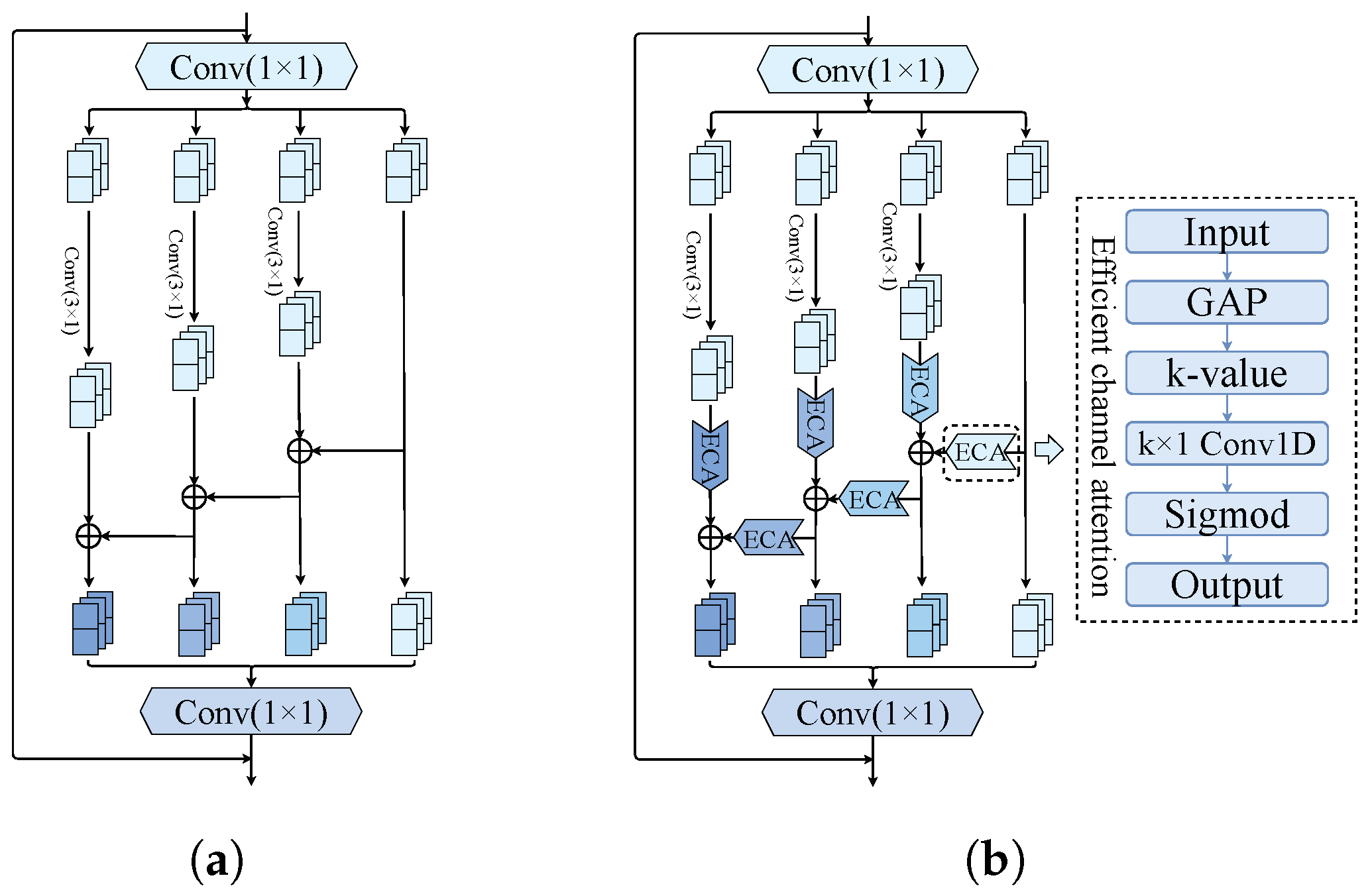
• An MFIR module is designed. This module uses multiple small convolution kernels to construct a multiscale residual module through a hierarchical structure. This design enables us to generate feature combinations with varying numbers, sizes, and scales of receptive fields. The equivalent receptive fields are larger, and richer features can be acquired than using the same number of convolution kernels. This module not only realizes the feature interaction between different scales, but also purifies the feature expression through the ECA mechanism;
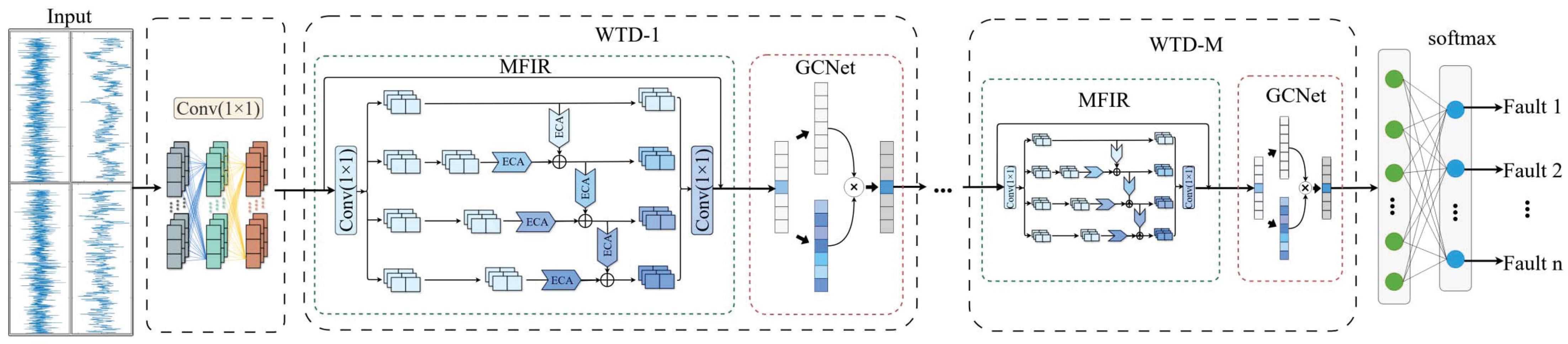
• A WTD sub-network is proposed. By integrating the MFIR module with the GCNet, a unified model is established to capture local and global characteristics. The output features of this sub-network contain both the multiscale information and the wide temporal dependencies. Compared with traditional multiscale methods and temporal modeling methods, the WTD sub-network can provide richer and more discriminative feature representations for industrial process fault diagnosis.

The paper is organized as follows. Section 2 introduces the relevant works of multiscale feature extraction and the capture of wide temporal dependency. Section 3 elaborates on the proposed MIPGC-Net for fault diagnosis. Section 4 presents the experimental setting and discusses the results from two different industrial process. Section 5 summarizes the conclusions.

2. Related Works

This section covers the methods of extracting multiscale features and capturing wide temporal dependencies.

2.1. Multiscale Feature Extraction

Industrial production processes usually encompass multiple operational units spanning varying time and frequency scales [27]. During the running process, variables, such as temperature, pressure, and flow rate, are influenced by diverse events, resulting in different patterns and changes across different time or frequency scales. Furthermore, different measurement instruments vary in temporal resolution and sampling frequency when processing these variables. For example, real-time pressure and temperature monitoring requires a fast response, whereas equipment condition monitoring usually spans longer periods. In large industrial furnaces, temperature changes occur relatively slowly, so temperature sensors are sampled at a low frequency with time resolutions in seconds or minutes. While the vibration monitoring of equipment such as bearings requires high-speed sampling due to rapid vibration changes, the time resolution of vibration sensors is usually in the microsecond or millisecond range.

To address the multiscale problem, many scholars have explored various approaches. Huang et al. introduced a multiscale cascade CNN, which uses kernels with varying sizes for feature extraction [28]. Song et al. developed a fault diagnosis method combining multiscale CNN with a matrix diagram [29]. Yin et al. proposed a multiscale low-rank convolutional autoencoder (MLRCAE) [30]. Zhao et al. proposed an adaptive multiscale CNN by constructing three parallel convolutional pathways [31]. Similarly, Liu et al. presented a multiscale CNN with three parallel branches and each branch used different kernel sizes [32]. These methods extract multiscale features by setting different convolution kernel sizes. Although different kernel sizes can provide diverse feature expressions, using more training parameters poses challenges in model training and the actual receptive field is still not enough. In addition, the parallel branch design limits feature interactions between different pathways. Overall, the existing multiscale methods for fault diagnosis face issues of high computational demands and insufficient feature interaction between parallel convolutional pathways. The proposed MFIR module in this paper has a skip connection architecture-like residual network, which help to reduce the computational complexity. Moreover, the ECA mechanism is introduced at each scale and between scales, enhancing feature interaction across pathways while reducing irrelevant information and refining feature expression.

2.2. Capture of Wide Temporal Dependency

In the industrial production process, due to the closed-loop control system and the high-speed sampling of equipment, process data usually present temporal correlations [14]. On the one hand, the current process state is influenced by the historical state. On the other hand, certain events occurring at an early stage may have long-term and persistent effects. For example, in a chemical reaction, rapid temperature changes in the reactor prompt the control system to adjust heating or cooling in order to stabilize temperatures. However, temperature fluctuations may alter the timing of certain critical chemical reactions, accelerating or delaying them. This may potentially affect subsequent reaction products, thereby impacting product quality and even persisting across multiple production cycles. Therefore, from the perspective of global historical data, the wide temporal dependencies exist in industrial process data.

To capture wide temporal dependencies of process data and enhance feature expression, many scholars have conducted research, such as LSTM, Transformer, and hybrid models. Chadha et al. introduced a bidirectional LSTM fault diagnosis approach for time sequential data, providing a viewpoint change and enabling one to classify faults over longer temporal sequences [33]. Zhang et al. presented an LSTM-based stacked denoising autoencoder (LSTM–SDAE) method, which can capture the multivariate temporal correlation information of the wind turbine system [34]. A CNN–LSTM hybrid model for fault diagnosis is presented by Zhao et al., combining an adaptive multiscale CNN with the enhanced highway LSTM (ACEL) to address limitations of CNNs in capturing wide temporal dependencies [31]. Wu et al. developed a Transformer-based method for detecting and diagnosing the faults of vibration signals. This method distinguishes different known fault types and also has the ability to detect novel unknown faults through Mahalanobis distance [35]. Zhao et al. introduced an attention-based LSTM fault diagnosis approach, which uses the bidirectional LSTM to capture temporal dependencies and adopts the attention mechanism to generate weights to emphasize important fault information [36]. Deng et al. presented an anomaly detection approach with interpretability, graph deviation network (GDN), by combining the graph neural network (GNN) and attention mechanism, to deal with multivariate time-series data on the secure water treatment dataset [37]. Although these time-series analysis models have more advantages than CNN in processing time sequential data, they usually require higher computational cost. In addition, these methods still face limitations when extracting multiscale features and realizing feature interaction purification.

To enable CNNs to capture global information, some scholars have improved the backbone CNN architectures to overcome the limitation that convolution operations are restricted to local neighborhoods. Wang et al. introduced a non-local network (NLNet) with a self-attention mechanism, which effectively captures the relationships between elements in both spatial and temporal sequences [38]. Cao et al. observed that NLNet tends to generate similar global contexts regardless of the query locations in the input, so a query-independent modified method was proposed as an improvement over NLNet [39]. This simplified network is known as the global context network, which ensures global information while also reducing computational complexity. Subsequently, many researchers conducted research on this basis. Lyu et al. proposed the RSG method by combining residual unit, soft threshold, and global contexts, and applied it to diagnosing faults in motor bearings [40]. Tong et al. introduced a residual global context shrinkage network (RGNet) to identify the faults in rotating machinery [41]. Xia et al. used GCNet to capture wide temporal dependencies and proposed the global temporal block (GTB) [42]. The GTB is combined with a temporal convolutional network (TCN) to capture overall feature tendency and predict the remaining useful life (RUL) for turbine engines. Therefore, we propose a WTD sub-network by integrating the proposed MFIR module with GCNet to establish a unified model of local multiscale features and global temporal features. With this design, the WTD sub-network can effectively obtain the wide temporal dependencies from process data, making up for the deficiency of traditional CNN in global information extraction, thereby obtaining more comprehensive feature expression.

3. Proposed Method

This section presents a comprehensive explanation of MIPGC-Net. Firstly, we propose the MFIR module to obtain multiscale features from input by utilizing interconnected pathways and the ECA mechanism. Then, the WTD sub-network is proposed by integrating the MFIR module with GCNet to further capture wide temporal dependencies. Lastly, MIPGC-Net is introduced by integrating local information with global contexts, achieving more comprehensive and discriminative representations for industrial process fault diagnosis.

3.1. MFIR Module

The MFIR module is depicted in Figure 1. Firstly, a simple multiscale residual module (simple MS) is used as the basic framework and the interaction mechanism is introduced to construct a multiscale feature interaction module (MFI). As shown in Figure 1a, after the $1\times 1$ convolution, we split the feature maps into S subsets, corresponding to the groups of squares in the first row, denoted by ${x_{MS}}_i$, where $i\in \{1,2,\dots ,S\}$. Every subset ${x_{MS}}_i$ corresponds to one pathway and these subsets have the same channel size, which is $1/S$ of the input feature map. Except for ${x_{MS}}_1$, each ${x_{MS}}_i$ undergoes processing through a $3\times 1$ convolution, denoted by $K_i(·)$. We represent the output of every pathway by ${y_{MS}}_i$, corresponding to the groups of squares in the last row in Figure 1a. The previous output ${y_{MS}}_{i-1}$ is added to the output of $K_i(·)$ to obtain the current output ${y_{MS}}_i$, and ${y_{MS}}_i$ is then passed to the next pathway. In this way, features from different pathways can interact and fuse with each other. In order to reduce parameters, the $3\times 1$ convolution of ${x_{MS}}_1$ is omitted. Thus, ${y_{MS}}_i$ can be written as

$${y_{MS}}_i=\left\{\begin{array}{cc}{x_{MS}}_i\hfill & \mathrm{if}i=1\hfill \\ K_i\left({x_{MS}}_i\right)+{y_{MS}}_{i-1}\hfill & \mathrm{if}2\le i\le S.\hfill \end{array}\right.$$

(1)

In the multiscale residual module, the pathways are organized as a hierarchical structure to achieve the efficient interaction of multiscale features. Whenever a feature split ${x_{MS}}_i$ passes through the $3\times 1$ convolution kernel, ${y_{MS}}_i$ can achieve a larger equivalent receptive field. Because of the combinatorial explosion effect, this multiscale residual module can generate feature combinations with varying scales of receptive fields. Meanwhile, since pathways are interconnected, features at different scales can perform feature interaction, resulting in more abundant multiscale features.

Since the equivalent receptive field increases, the network extracts more features. At this point, it is necessary to introduce the ECA mechanism to reduce irrelevant information and refine feature expression. The ECA mechanism uses 1-D convolution to model inter-channel relationships in the input, generating channel weights adaptively. These weights are then applied to the original features, enhancing important channels while suppressing irrelevant information, thereby improving the feature expression. Then, the MFIR module proposed is shown in Figure 1b. Except for ${x_{MS}}_1$, the feature subset from every pathway first passes through a $3\times 1$ convolution operator and then goes through an ECA operation. The ECA operation corresponding to the input ${x_{MS}}_i$ is denoted by $E_i(·)$. The ECA operation is also performed between pathways, which is denoted as $E_{i-1,i}(·)$. The outputs of $E_i(·)$ and $E_{i-1,i}(·)$ are added and then fed into ${y_{ME}}_i$. This process is repeated multiple times until every input feature map has been processed. Thus, ${y_{ME}}_i$ can be written as

$$\begin{array}{cc}\hfill {y_{ME}}_i& =\mathrm{MFIR}\left({x_{MS}}_i\right)\hfill \\ \hfill & =\left\{\begin{array}{cc}{x_{MS}}_i\hfill & \mathrm{if}i=1\hfill \\ E_i\left[K_i\left({x_{MS}}_i\right)\right]+E_{i-1,i}\left({y_{ME}}_{i-1}\right)\hfill & \mathrm{if}2\le i\le S.\hfill \end{array}\right.\hfill \end{array}$$

(2)

The calculation process of the ECA mechanism is as follows. Firstly, we apply the global average pooling (GAP) to the input of a certain layer. Then, the 1-D convolution with a kernel size of k is employed to capture the interaction information across channels, considering every channel and its k neighbors. Next, a sigmoid activation function is employed for obtaining channel weights. Finally, these weights are applied to the input. Here, the kernel size k is decided by the dimension C of the channel, as shown in Equation (3), where ${\left|t\right|}_{odd}$ is the closest odd integer to t. In this paper, the values of $\gamma$ and $\beta$ are chosen as 2 and 1.

$$k=\psi \left(C\right)={\left|{\displaystyle \frac{{log}_2\left(C\right)}{\gamma }}+{\displaystyle \frac{\beta }{\gamma }}\right|}_{odd}.$$

(3)

The output ${y_{ME}}_i$ of each scale is concatenated and this operation is noted as $Cat(·)$. Then, the $1\times 1$ convolution is used to obtain the output of the MFIR module, which is denoted as $y_{MFIR}$.

Overall, the proposed MFIR module is designed with a multiscale structure to extract multiscale features from process data. Multiple $3\times 1$ small convolution kernels are used to extract multiscale features. Compared to larger kernels, the small convolution kernels require less calculation. The hierarchical connections between pathways enhance feature interactions, resulting in more abundant feature information. Moreover, this module introduces the ECA mechanism to increase the weight of important features while reducing information redundancy, thereby refining feature expression. Additionally, the module has a skip connection structure, similar to that in residual networks (ResNet), which helps to prevent vanishing gradient and reduces computational costs.

3.2. WTD Sub-Network

In industrial process fault diagnosis, time sequential data usually have temporal dependencies. Accurately capturing the temporal dependencies from the input is essential for identifying progressive faults and anomalous patterns with long-term evolution. However, there is an inherent limitation of traditional CNN. Convolutional operation is essentially a local operation that mainly relies on multiple convolutional kernels within the local receptive fields to extract features. This makes it difficult for the network to capture the global context information from the data, especially the effects between distant time points in industrial process data. To handle this deficiency, we propose the WTD sub-network, as presented in Figure 2. This sub-network combines the proposed MFIR module with the GCNet, forming a unified network that effectively captures multiscale local features and global contexts. The output $y_{MFIR}$ from the MFIR module is fed into GCNet to obtain the wide temporal dependencies from the input feature map.

The architecture of GCNet is depicted in Figure 3. The input of GCNet is $y_{MFIR}$, and $y_{WTD}$ denotes the output. Both $y_{MFIR}$ and $y_{WTD}$ have the same dimensions, defined as $C\times F$. Here, C stands for the quantity of channels. F is the data length of each channel. The transformation matrices $W_k$, $W_{v_1}$, and $W_{v_2}$ are $1\times 1$ convolution layers. Taking $y_{MFIR}={\left\{{y_{MFIR}}_i\right\}}_{i=1}^F$ as an example of the input, F denotes the position number. The core of GCNet is to obtain global context information of the input through the global attention mechanism, which compensates the limitation of traditional CNN in the local receptive field. First, the softmax function is employed to generate attention weights between the input feature map ${y_{MFIR}}_i$ and the global contexts. Then, the features are aggregated according to the attention weights to obtain the context features. Next, through the bottleneck transformation (including layer normalization and ReLU activation), the transformed result is fused with the input ${y_{MFIR}}_i$ to produce the output feature map $y_{WTD}$. In this case, the bottleneck ratio r is set to 16. The output of the WTD sub-network is computed as

$$\begin{array}{cc}\hfill {y_{WTD}}_i& =\mathrm{GC}\left({y_{MFIR}}_i\right)\hfill \\ \hfill & ={y_{MFIR}}_i+W_{v_2}\mathrm{ReLU}\left(\mathrm{LN}\left(W_{v_1}\sum _{j=1}^F{\omega }_j{y_{MFIR}}_j\right)\right).\hfill \end{array}$$

(4)

Here, the variable i serves as the index for query locations, and j refers to all available positions in global contexts. ${\omega }_j={\displaystyle \frac{e^{W_k{y_{MFIR}}_j}}{{\sum }_{f=1}^F{e}^{W_k{y_{MFIR}}_f}}}$ denotes the global attention pooling weight. $\mathrm{LN}(·)$ is layer normalization, and $\mathrm{ReLU}(·)$ denotes the ReLU activation function. With this design, the WTD sub-network can effectively capture the wide temporal dependencies in industrial process data, which makes up for the deficiency of traditional CNN in global information acquisition.

Figure 3. Architecture of GCNet.

Figure 3. Architecture of GCNet.

3.3. MIPGC-Net Method for Fault Diagnosis

Industrial processes may experience multiple types of faults. Diagnosing faults for various health conditions can be considered as a multi-classification problem. The MIPGC-Net method for industrial process fault diagnosis is proposed by stacking multiple WTD sub-networks. The training process is illustrated through Figure 4 and Algorithm 1.

For the input sample $X=\{x_1,x_2,\dots ,x_N\}$, a set of regular 1-D convolutions are used, denoted as $Conv(·)$. The primary purpose is to adjust the channel size of the input feature maps so as to match the need to split the feature map subsets in the subsequent MFIR module. Also, it can be seen as a preliminary feature extraction. Next, to extract multiscale features, we propose the MFIR module. Specifically, the feature maps are split into S subsets, ${x_{MS}}_i$, each with the same channel size. The pathways are interconnected as a hierarchical structure and the ECA mechanism is applied to every pathway as well as at the pathway junctions. The module not only can extracts multiscale features but also prevents feature redundancy, enabling the effective interaction and refinement of features.

Algorithm 1 MIPGC-Net training process for industrial process fault diagnosis.

Input:  The training set $X=\{x_1,x_2,\dots ,x_k,\dots ,x_N\}$, initial network parameters ${\theta }_{MIPGC-Net}$, the number of iterations for one epoch B; Output:  Optimized parameters ${\Theta }_{MIPGC-Net}$.   1: while network parameters not converged do   2:     $x_{MS}\leftarrow Conv\left(x_k\right)$;   3:     for $i=1$ to B do   4:         for $i=1$ to M do   5:             while j in scales do   6:                 ${y_{ME}}_{i,m,j}$←${\mathrm{MFIR}}_j\left({x_{MS}}_{i,m,j}\right)$;   7:                 ${y_{MFIR}}_{i.m}$←$Cat\left(\sum {y_{ME}}_{i,m,j}\right)$;   8:             end while   9:             ${y_{WTD}}_{i,m}$←$\mathrm{GC}\left({y_{MFIR}}_{i,m}\right)$; 10:         end for 11:         $P_j$←$\mathrm{softmax}\left(\mathrm{FC}\left({y_{WTD}}_{i,M}\right)\right)$; 12:         ${\Theta }_{MIPGC-Net}$←$arg{min}_{{\theta }_{MIPGC-Net}}\left(\mathrm{Loss}\left(R_j,P_j\right)\right)$; 13:    end for 14: end while 15: return ${\Theta }_{MIPGC-Net}$.

Next, the WTD sub-network is proposed. Because CNNs primarily use multiple convolution kernels to extract features and convolution is a local operation, they tend to overlook the global information of the input, specifically the wide temporal dependencies of process data. Therefore, by combining the MFIR module with GCNet, the WTD sub-network is designed to capture the wide temporal dependencies.

Then, m WTD sub-networks are stacked to extract features. Assuming that the output of the last WTD sub-network is ${y_{WTD}}_M$, it is expanded into a feature vector using the fully connected layer, denoted as $\mathrm{FC}(·)$. Then, the feature vector undergoes a softmax operation, denoted as $\mathrm{softmax}(·)$, to yield a probability distribution. Therefore, we have

$$Q=\mathrm{FC}\left({y_{WTD}}_M\right),$$

(5)

$$P=\mathrm{softmax}\left(Q\right).$$

(6)

After that, the model parameters are trained by backpropagation on the training dataset with the cross-entropy loss as the optimal objective. The loss function, as presented in Equation (7), is calculated between the prediction P and the truth label R for N samples.

Finally, the testing dataset is utilized to carry out fault diagnosis. With the integration of the MFIR modules into the network, MIPGC-Net achieves the feature interaction and refinement, obtaining more abundant multiscale information while purifying feature expression. Also, through the use of the WTD sub-networks, MIPGC-Net captures wide temporal dependencies, resulting in a richer feature representation.

$$\begin{array}{cc}\hfill L& =\mathrm{Loss}(R,P)\hfill \\ \hfill & =-{\displaystyle \frac{1}{N}}\sum _{i=1}^{N}RlogP.\hfill \end{array}$$

(7)

4. Experiments and Discussion

The Tennessee Eastman (TE) process and the Continuous Stirred-Tank Reactor (CSTR) process are employed to verify the validity and advantages of the proposed method. As a well-known benchmark for industrial fault diagnosis research, the TE process presents a simulated case of an actual production process. This study adopts the extended TE dataset proposed by Rieth et al. in 2017, which is available from the Harvard repository [43]. The dataset consists of four subsets, including the normal training, normal testing, fault trainings and fault testing datasets, with 500 simulation experiments conducted for each subset. Every time sequential example contains 52 variables, which are sampled every 3 min from the running process. The training dataset has a sampling duration of 25 h. The testing dataset runs 48 h. In the training dataset, faults are introduced after 1 h, whereas, in the testing dataset, the faults are generated after 8 h. The dataset includes normal data (numbered 0) and 20 types of fault information (numbered 1 to 20). Moreover, the CSTR process and the related experiments are thoroughly introduced in Section 4.5.

4.1. Evaluation Metrics

To assess the method effectiveness, we employ two commonly adopted statistical indicators, accuracy (ACC) and F1-score [19,33], which are formulated as

$$\mathrm{ACC}={\displaystyle \frac{\mathrm{TP}+\mathrm{TN}}{\mathrm{TP}+\mathrm{TN}+\mathrm{FP}+\mathrm{FN}}},$$

(8)

$$\mathrm{F}1\text{-}\mathrm{score}={\displaystyle \frac{2\times \mathrm{Precision}\times \mathrm{Recall}}{\mathrm{Precision}+\mathrm{Recall}}}.$$

(9)

Here, $\mathrm{Precision}=\mathrm{TP}/(\mathrm{TP}+\mathrm{FP})$ and $\mathrm{Recall}=\mathrm{TP}/(\mathrm{TP}+\mathrm{FN})$. In fault diagnosis, we regard accurately classified cases as positive and others as negative. True positive (TP) presents the count of accurately classified fault samples. False negative (FN) indicates the count of fault samples in a certain category that are predicted to be faults in other categories. TN and FP correspond to the count of true negative and false positive samples, respectively. ACC denotes the correct classification rate among all instances. As the harmonic mean of Recall and Precision, the F1-score balances the FP and FN classified samples.

Also, we evaluate the method performance by training time per epoch, inference time per sample, the count of model parameters (Params), and floating point operations per sample (Flops). T-distributed stochastic neighbor embedding (t-SNE) is adopted for comparing feature extraction capabilities of various methods, including the quantitative metrics of Kullback–Leibler (KL) divergence, silhouette scores, and Davies–Bouldin index.

4.2. Experiment Setting

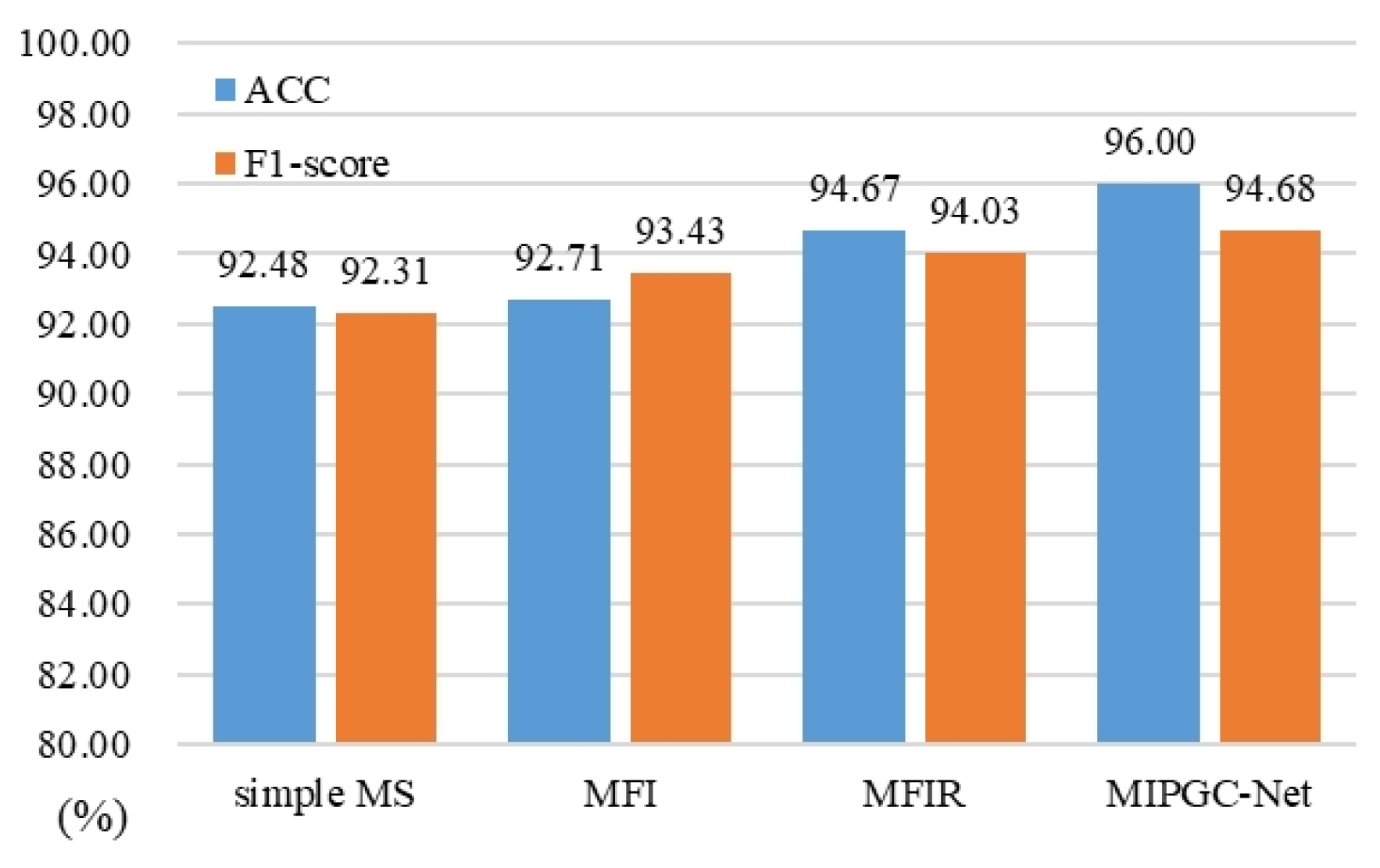
In the experiment, the WTD sub-network is stacked four times, so the network includes four MFIR layers and four GCNet layers. The MFIR module involves two hyperparameters, the scale number s and the width w, which are determined experimentally. The convolution kernel size used in the network is $3\times 1$. Experiments are conducted under consistent conditions, varying only the settings for s and w. The search is performed with a step size of 2, setting s and w to values of 2, 4, …, and 12. All experiments are executed using PyTorch 1.13.0, NVIDIA P100 GPU 16GB, and Intel(R) Xeon(R) @ 2.00 GHz.

Table 1. Hyperparameter selection.

Scale	Width	ACC	F1-Score	Time(s)	Scale	Width	ACC	F1-Score	Time(s)
2	2	0.8774	0.8679	190	8	2	0.9463	0.9337	355
	4	0.9407	0.9284	361		4	0.9528	0.9398	548
	6	0.9537	0.9412	750		6	0.9527	0.9401	977
	8	0.9491	0.9367	1233		8	0.9558	0.9428	1528
	10	0.9552	0.9424	1859		10	0.9502	0.9373	2271
	12	0.9531	0.9412	2730		12	0.9558	0.9436	3222
	Avg	0.9382	0.9263	1788		Avg	0.9523	0.9396	1484
4	2	0.9367	0.9266	248	10	2	0.9503	0.9377	400
	4	0.9488	0.9363	437		4	0.9535	0.9408	651
	6	0.9466	0.9340	885		6	0.9527	0.9399	1109
	8	0.9537	0.9419	1385		8	0.9501	0.9374	1699
	10	0.9576	0.9449	1972		10	0.9549	0.9424	2440
	12	0.9499	1.9370	2852		12	0.9539	0.9412	3466
	Avg	0.9489	0.9368	1297		Avg	0.9526	0.9399	1628
6	2	0.9473	0.9346	281	12	2	0.9473	0.9349	419
	4	0.9476	0.9348	478		4	0.9539	0.9408	693
	6	0.9600	0.9468	934		6	0.9546	0.9420	1209
	8	0.9535	0.9409	1415		8	0.9568	0.9435	1799
	10	0.9523	0.9401	2107		10	0.9539	0.9412	2623
	12	0.9524	0.9397	3075		12	0.9523	0.9391	3715
	Avg	0.9522	0.9395	1382		Avg	0.9531	0.9403	1743

presents the results of hyperparameter selection.

For every s, the experimental results under different w values are averaged. The average results indicate that, as s increases, both ACC and F1-score improve, but training time also increases. Also, regardless of the scale number s, the training time grows significantly with the rising value of w. ACC and F1-score initially rise as w increases, but, after reaching the best, they start to decline. This demonstrates that increasing either s or w leads to higher computational costs and longer training time, with w contributing to a particularly substantial increase. Within acceptable training time, the larger s value can obtain higher accuracy, but w should be carefully selected.

Table 1 highlights the optimal ACC and F1-score results for every scale, corresponding to the s–w combinations of 2–10, 4–10, 6–6, 8–12, 10–10, and 12–8, respectively. The 6–6 combination records the top ACC and F1-score, with the shortest training time of 934 s. Thus, the subsequent experiments are conducted using this combination.

When the hyperparameters are set to the s–w = 6–6 combination, Figure 5 presents a confusion matrix of fault diagnosis using MIPGC-Net. Overall, different faults can be distinguished and fewer samples are misclassified. To provide a more comprehensive assessment, additional experiments are performed, including the ablation study and comparison with other methods.

4.3. Ablation Study

To evaluate the method performance, MIPGC-Net is compared with four variant experiments. The first variant is the simple multiscale residual network (simple MS), which does not have feature interaction refinement mechanism. The second one retains the feature interaction but removes the ECA mechanism from the network, referred to as multiscale feature interaction network (MFI). The third experiment employs the MFIR module presented in this paper, and the fourth is MIPGC-Net.

The results can be observed in Figure 6. Figure 6a presents the ACC results. Figure 6b displays the F1-score results. For both ACC and F1-score, there is little difference between the four experiments on Faults 1 to 7. The results indicate that using the proposed MFIR module or the MIPGC-Net method can improve both ACC and F1-score across nearly all fault types, especially for Faults 8, 10, 12, 13, 16, 17, and 18.

In general, when compared with variant experiments, we show that the feature interaction refinement mechanism of the proposed MFIR module can help to extract more effective features. As with integrating wide temporal dependencies in the network, the proposed MIPGC-Net method demonstrates superior performance in fault diagnosis.

Figure 7 shows the average diagnosis results across several faults in the TE process. As a whole, the MFI method shows improvement over the simple MS method, indicating that feature interaction across scales helps to capture richer feature information. Compared to MFI, the proposed MFIR module further enhances performance, with ACC increasing by 1.90% and F1-score by 0.6%. This improvement demonstrates that the attention mechanism introduced in the module effectively emphasizes important features while suppressing irrelevant information. Thus, it verifies the effectiveness of the MFIR module for feature extraction. Furthermore, MIPGC-Net achieves even better results than MFIR, indicating that the WDT sub-network in MIPGC-Net obtains the wide temporal dependencies of process data, leading to more comprehensive feature information.

Among the four experiments, MIPGC-Net has the highest ACC and F1-score, with ACC at 96.00% and F1-score at 94.68%. Compared with the simple MS method, the proposed MIPGC-Net method improves ACC by 3.50% and F1-score by 2.37%. This confirms that the MIPGC-Net method is highly effective for industrial process fault diagnosis.

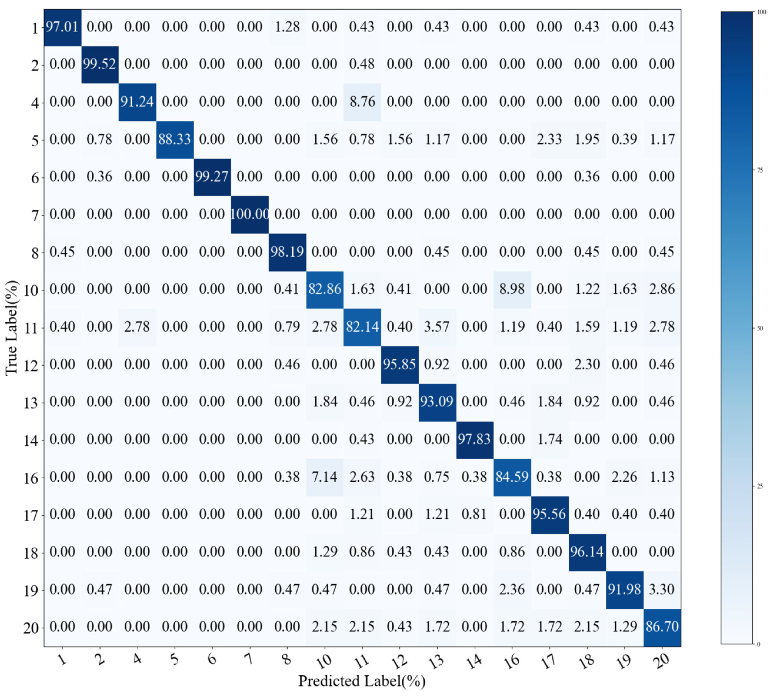
4.4. Comparison Study in the TE Process

To further evaluate the superiority, we compare the MIPGC-Net proposed with other methods. Since MIPGC-Net uses CNNs as its backbone and incorporates a ResNet structure within the MFIR module, two typical deep learning methods CNN and ResNet are selected for comparison. In these experiments, the network layers and convolution kernel size are consistent with those used in our method. In addition, given that LSTM, Transformer, and their improved hybrid methods have advantages in analyzing time sequential data, we compare these method, including Auto-LSTM [44], LSTM–LAE [16], ACEL (CNN–LSTM method) [31], Transformer [35], and Att-LSTM (attention-based LSTM method) [36]. In

Table 2. Fault diagnosis results compared to other methods in the TE process.

Faults	CNN		ResNet		Auto-LSTM		LSTM-LAE		ACEL		Transformer		Att-LSTM		MIPGC-Net
	ACC	F1-Score	ACC	F1-Score	ACC	F1-Score	ACC	F1-Score	ACC	F1-Score	ACC	F1-Score	ACC	F1-Score	ACC	F1-Score
1	98.80	99.34	99.15	99.57	99.00	99.38	99.33	99.27	99.27	99.52	100.00	97.50	99.31	98.28	99.29	99.26
2	99.06	99.53	99.02	99.51	98.88	99.29	99.34	99.63	99.21	99.58	98.73	98.94	97.85	98.54	98.60	98.77
4	98.52	93.91	90.94	93.98	98.52	95.37	97.31	95.60	97.51	96.59	98.76	96.18	99.02	95.86	97.38	96.19
5	97.97	97.87	94.50	97.15	98.75	98.82	98.41	98.95	98.82	99.37	100.00	97.74	99.20	98.76	99.45	98.89
6	98.70	99.35	99.46	99.73	99.83	99.92	98.96	99.48	99.25	99.62	100.00	99.82	100.00	100.00	100.00	100.00
7	99.76	99.70	99.80	99.90	99.25	99.62	99.70	99.81	99.62	99.79	100.00	99.76	100.00	100.00	100.00	100.00
8	91.94	92.31	98.25	96.05	94.66	95.56	91.59	93.77	96.27	96.73	96.20	97.31	88.63	91.38	98.66	96.29
10	62.87	72.45	89.35	91.44	82.38	83.97	86.02	84.08	86.05	82.27	86.23	86.59	85.63	86.06	89.17	89.09
11	71.25	78.57	90.69	87.86	80.57	85.97	81.64	85.69	85.31	88.11	86.08	88.89	85.09	82.86	89.94	88.29
12	81.60	88.29	97.28	96.96	93.79	94.26	93.56	91.65	97.30	96.29	93.46	96.05	89.50	91.49	97.61	95.85
13	92.04	88.00	95.82	96.33	92.41	94.22	88.49	91.62	93.96	96.42	90.54	93.27	84.86	89.17	98.97	94.53
14	95.61	97.38	99.42	99.04	97.52	98.13	97.20	98.23	98.75	99.07	98.77	97.97	97.94	97.74	99.38	98.61
16	70.68	59.08	91.61	89.30	81.33	80.27	85.03	85.46	66.23	67.73	88.66	93.59	84.27	89.09	88.79	90.45
17	93.59	93.67	94.44	96.38	94.94	95.07	94.72	93.60	95.75	96.29	92.23	92.82	90.30	93.42	97.87	94.25
18	90.61	93.40	94.62	96.26	91.87	94.98	90.34	94.37	93.50	95.74	91.52	88.36	86.12	89.84	94.36	92.49
19	74.06	69.71	91.80	86.01	86.95	78.56	88.46	86.25	84.91	80.49	96.98	95.95	92.92	89.21	92.67	91.64
20	77.14	76.70	86.62	87.99	92.06	90.62	90.35	83.74	89.12	87.95	94.50	89.57	87.94	78.95	89.87	84.90
Avg	87.89	88.19	94.87	94.91	93.10	93.18	92.97	93.01	92.99	93.03	94.86	94.72	92.27	92.39	96.00	94.68

, the fault diagnosis results compared to other methods are provided in detail.

Compared to CNN, MIPGC-Net shows improvement, with an average ACC increase of 9.11%. Although both methods use convolution kernels to obtain abstract features of the input, the proposed method differs from CNN by considering multiscale features and temporal correlations of process data. The MFIR module in our method has a structure of interconnected pathways, effectively obtaining multiscale features. The WTD sub-network considers the global information by capturing the wide temporal dependencies of the process data. These enhancements contribute to the superior performance of MIPGC-Net for fault diagnosis.

Compared with ResNet, our method demonstrates better performance, with an average ACC improvement of 1.13%. This is attributed to the MFIR module, which not only has the skip connection like ResNet, but also extracts multiscale features. By using multiple small convolution kernels instead of a single kernel, the MIPGC-Net method enriches feature expression. In particular, the interconnection between pathways facilitates feature interaction, thereby enhancing feature richness. Furthermore, the introduced ECA mechanism helps to emphasize important features and refine feature expression.

Compared with Auto-LSTM, LSTM–LAE, ACEL, Transformer, and Att-LSTM, the proposed method is also competitive, with an average ACC improvement of 2.76%. Although these temporal modeling methods are effective in dealing with time sequential data, they neglect to extract the local information of the process data. In contrast, MIPGC-Net integrates both local multiscale feature and global wide temporal dependencies, thereby achieving more comprehensive feature expression and superior fault diagnosis performance.

Table 3. Fault diagnosis performance comparison in the TE process.

Index	CNN	ResNet	Auto-LSTM	LSTM-LAE	ACEL	Transformer	Att-LSTM	MIPGC-Net
Training time (s)	4.78	4.25	3.30	10.50	11.60	19.38	23.13	3.43
Inference time (μs)	2.56	4.25	3.20	1.80	1.71	13.50	12.31	4.89
Params (M)	1.04	3.85	3.30	2.14	2.60	1.66	4.04	3.07
Flops (M)	4.08	9.81	6.30	4.18	5.20	130.00	15.70	4.28
KL-divergence	1.09	1.11	0.50	0.61	0.94	0.63	1.72	0.50
Silhouette scores	0.29	0.48	0.49	0.43	0.37	0.52	0.27	0.52
Davies–Bouldin	1.87	0.93	0.96	1.35	1.16	0.89	1.49	0.77

shows the performance comparison in the TE process. In terms of model complexity, the proposed method has larger Params than CNN, LSTM–LAE, ACEL, and Transformer. However, regarding Flops, our method outperforms all of them except CNN. Although CNN has an advantage in both Params and Flops, the ACC is improved by 8.11% when using our method, reflecting a better balance between performance and complexity. Regarding computational efficiency, MIPGC-Net requires less training time than all the comparisons, except Auto-LSTM. For inference time, our method achieves 4.89 μs per sample. Although our results are not flawless, this time is sufficient to meet the real-time requirements of most industrial systems.

In summary, the proposed MIPGC-Net method proves to be effective for industrial process fault diagnosis, attaining a 3.29% average accuracy enhancement over the above seven methods. This improvement is primarily indebted to the ability of MIPGC-Net to simultaneously extract local multiscale features and global wide temporal dependencies of the process data, which results in more comprehensive and discriminative feature representations.

To evaluate the feature learning capabilities of different methods, t-SNE is used to create two-dimensional feature visualizations [45]. Figure 8 shows the feature distribution of the step faults. Figure 9 presents the feature visualization of the random, slow drift, and sticking faults, and Figure 10 corresponds to the unknown faults. Also, the quantitative results of KL-divergence, silhouette scores, and Davies–Bouldin index are presented in Table 3. KL-divergence measures class separability after feature extraction, with lower values indicating better separation. Silhouette scores evaluate the clustering effect: higher values mean better clusters. The Davies–Bouldin index evaluates cluster compactness, with lower values signifying more distinct and compact clusters. Compared with other methods, both the visualization and quantitative results demonstrate that MIPGC-Net exhibits competitive performance and outperforms other methods in fault diagnosis.

4.5. Comparison Study in the CSTR Process

CSTR is a commonly used reactor in polymerization chemical reactions. In the reactor, the reaction materials are continuously added at a constant flow rate, while the reaction products flow out at the same rate steadily. Through the action of the stirrer, the newly added materials can be fully mixed with the existing materials in the reactor. The reaction rate is mainly affected by the temperature and concentration of the material in the reactor, and the optimization of the reaction process can be realized through the precise control of these parameters.

As depicted in Figure 11, the CSTR process involves an irreversible exothermic reaction in which component A is converted to component B within the reactor. The process consists of nine measurement variables [46,47]. The samples are collected at an interval of 1 min and there are six fault patterns. The training dataset contains one normal and six fault datasets with 250 samples in each dataset. Each testing dataset has 500 samples. The fault occurs at the 151st sample and persists throughout the remainder of the process. A description of the faults can be found in

Table 4. Fault patterns of the CSTR process.

Faults	Descriptions	Magnitude
1	$C_{AA}$ step change	$1.0$ kmol/m3
2	$C_{AA}$ ramp change	$d{C}_{AA}/dt=0.2$ kmol/(m3· min)
3	$T_C$ random disturbance	$U(2,4)$
4	$k_0$ slow drift	$k_0(t+1)=0.996\times k_0\left(t\right)$
5	Heat exchanger fouling	$-120$ J/(min−2· K)
6	$Q_C$ random measured noise	$N(0,5)$

.

As shown in

Table 5. Fault diagnosis results compared to other methods in the CSTR process.

Faults	CNN		ResNet		Auto-LSTM		LSTM-LAE		ACEL		Transformer		Att-LSTM		MIPGC-Net
	ACC	F1-Score	ACC	F1-Score	ACC	F1-Score	ACC	F1-Score	ACC	F1-Score	ACC	F1-Score	ACC	F1-Score	ACC	F1-Score
1	100.00	100.00	100.00	100.00	100.00	100.00	100.00	100.00	100.00	99.72	100.00	100.00	100.00	100.00	100.00	100.00
2	100.00	95.24	99.71	95.88	100.00	91.86	98.00	95.28	100.00	92.59	100.00	94.98	99.14	91.32	100.00	97.36
3	87.71	93.31	87.71	93.31	80.57	89.24	88.00	92.63	81.43	89.76	85.14	91.98	35.43	51.67	92.00	95.69
4	98.57	98.43	99.14	97.61	95.71	97.67	96.00	97.96	99.43	98.72	96.57	97.97	87.14	74.94	98.57	98.43
5	99.43	99.71	99.71	99.86	99.71	99.86	99.71	99.86	99.14	99.57	99.71	99.57	99.43	99.71	99.71	99.86
6	100.00	98.87	99.43	98.86	99.71	96.81	100.00	95.89	100.00	99.29	99.43	96.13	100.00	93.58	100.00	98.87
Avg	97.62	97.59	97.62	97.59	95.95	95.91	96.95	96.94	96.67	96.61	96.81	96.77	86.86	85.20	98.38	98.37

, fault diagnosis results of the CSTR process reveal the exceptional performance of our method, achieving an ACC of 98.38% and F1-score of 98.37%, further validating the effectiveness of MIPGC-Net on different datasets.

Partial classification results for Fault 3 in the CSTR process are shown in Figure 12. The horizontal axis represents the samples. Different colors dots indicate different sample categories. The red color dots are the normal samples. The fault occurs at the 151st sample, but due to diagnostic latency, some initial samples remain classified as normal. As the diagnostic method takes effect, Fault 3 is correctly identified as brown dots, while misclassified samples in other colors. The method, CNN, ACEL, and MIPGC-Net can diagnose the fault at the 156th sample, while other methods diagnose the fault at a later time. Moreover, the proposed method has fewer misclassifications than the others.

In general, comprehensive experimental results confirm the diagnostic effectiveness of the proposed MIPGC-Net in both TE and CSTR processes. The method exhibits strong generalization potential for fault diagnosis tasks in diverse industrial scenarios.

5. Conclusions

This work proposes a novel method, MIPGC-Net, for industrial process fault diagnosis. The MFIR module proposed is an efficient multiscale feature extraction module. This module employs a hierarchical connection structure between pathways and incorporates the ECA mechanism, which facilitates the effective interaction and refinement of multiscale features, enhancing feature richness and placing greater emphasis on critical features. To overcome the limitations of CNN in capturing global information, the WTD sub-network is designed by combining the MFIR module with the GCNet, forming a unified framework of simultaneously capturing multiscale local features and global context information. Based on this, MIPGC-Net is constructed for industrial process fault diagnosis. Compared with traditional temporal modeling methods, such as LSTM and Transformers, MIPGC-Net reduces inference latency while maintaining high accuracy, rendering it particularly appropriate for industrial fault diagnosis applications that demand real-time performance. Furthermore, comprehensive validation has been conducted on the TE and CSTR datasets, demonstrating that MIPGC-Net has strong generalization ability and can be applied to other time sequential analysis tasks, making it applicable to a wider range of industrial scenarios.

Nevertheless, there are some limitations in this paper. As a black-box model, MIPGC-Net is deficient in decision interpretability and cannot directly provide fault root causes. In addition, although explicit dimension transformation is avoided through the ECA mechanism and the bottleneck design of GCNet maintains the lightweight property, this study mainly focuses on enhancing the feature representation capability. In the future, we will further explore the design of interpretable and lightweight models.

References

1. Ma, Y.; Shi, H.; Tan, S.; Song, B.; Tao, Y. Semi-Supervised Relevance Variable Selection and Hierarchical Feature Regularization Variational Autoencoder for Nonlinear Quality-Related Process Monitoring. IEEE Trans. Instrum. Meas. 2023, 72, 3536711. [Google Scholar] [CrossRef]
2. Yu, E.; Luo, L.; Peng, X.; Tong, C. A multigroup fault detection and diagnosis framework for large-scale industrial systems using nonlinear multivariate analysis. Expert Syst. Appl. 2022, 206, 117859. [Google Scholar] [CrossRef]
3. He, Y.; Li, K.; Zhang, N.; Xu, Y.; Zhu, Q. Fault diagnosis using improved discrimination locality preserving projections integrated with sparse autoencoder. IEEE Trans. Instrum. Meas. 2021, 70, 3527108. [Google Scholar] [CrossRef]
4. Yu, F.; Liu, J.; Liu, D. Multimode Process Monitoring Based on Modified Density Peak Clustering and Parallel Variational Autoencoder. Mathematics 2022, 10, 2526. [Google Scholar] [CrossRef]
5. Li, Z.; Tian, L.; Jiang, Q.; Yan, X. Fault diagnostic method based on deep learning and multimodel feature fusion for complex industrial processes. Ind. Eng. Chem. Res. 2020, 59, 18061–18069. [Google Scholar] [CrossRef]
6. Zhou, K.; Wang, R.; Tong, Y.; Wei, X.; Song, K.; Chen, X. Domain generalization of chemical process fault diagnosis by maximizing domain feature distribution alignment. Process Saf. Environ. Prot. 2024, 185, 817–830. [Google Scholar] [CrossRef]
7. Yu, W.; Zhao, C. Broad convolutional neural network based industrial process fault diagnosis with incremental learning capability. IEEE Trans. Ind. Electron. 2020, 67, 5081–5091. [Google Scholar] [CrossRef]
8. Chen, Z.; Ke, H.; Xu, J.; Peng, T.; Yang, C. Multichannel Domain Adaptation Graph Convolutional Networks-Based Fault Diagnosis Method and With Its Application. IEEE Trans. Ind. Inform. 2023, 19, 7790–7800. [Google Scholar] [CrossRef]
9. Yang, F.; Tian, X.; Ma, L.; Shi, X. An optimized variational mode decomposition and symmetrized dot pattern image characteristic information fusion-Based enhanced CNN ball screw vibration intelligent fault diagnosis approach. Measurement 2024, 229, 114382. [Google Scholar] [CrossRef]
10. Yu, F.; Liu, J.; Liu, D.; Wang, H. Supervised convolutional autoencoder-based fault-relevant feature learning for fault diagnosis in industrial processes. J. Taiwan Inst. Chem. Eng. 2022, 132, 104200. [Google Scholar] [CrossRef]
11. Guo, X.; Guo, Q.; Li, Y. Dual-noise autoencoder combining pseudo-labels and consistency regularization for process fault classification. Can. J. Chem. Eng. 2024, 103, 1853–1867. [Google Scholar] [CrossRef]
12. Tian, W.; Liu, Z.; Li, L.; Zhang, S.; Li, C. Identification of abnormal conditions in high-dimensional chemical process based on feature selection and deep learning. Chin. J. Chem. Eng. 2020, 28, 1875–1883. [Google Scholar] [CrossRef]
13. Wang, Y.; Pan, Z.; Yuan, X.; Yang, C.; Gui, W. A novel deep learning based fault diagnosis approach for chemical process with extended deep belief network. ISA Trans. 2020, 96, 457–467. [Google Scholar] [CrossRef] [PubMed]
14. Zhang, S.; Bi, K.; Qiu, T. Bidirectional Recurrent Neural Network-Based Chemical Process Fault Diagnosis. Ind. Eng. Chem. Res. 2020, 59, 824–834. [Google Scholar] [CrossRef]
15. Zhang, Y.; Zhou, T.; Huang, X.; Cao, L.; Zhou, Q. Fault diagnosis of rotating machinery based on recurrent neural networks. Measurement 2021, 171, 108774. [Google Scholar] [CrossRef]
16. Zhang, S.; Qiu, T. Semi-supervised LSTM ladder autoencoder for chemical process fault diagnosis and localization. Chem. Eng. Sci. 2022, 251, 117467. [Google Scholar] [CrossRef]
17. Qin, R.; Lv, F.; Ye, H.; Zhao, J. Unsupervised transfer learning for fault diagnosis across similar chemical processes. Process Saf. Environ. Prot. 2024, 190, 1011–1027. [Google Scholar] [CrossRef]
18. Wang, C.; Zhang, Y.; Zhao, Z.; Chen, X.; Hu, J. Dynamic model-assisted transferable network for liquid rocket engine fault diagnosis using limited fault samples. Reliab. Eng. Syst. Saf. 2024, 243, 109837. [Google Scholar] [CrossRef]
19. Jia, L.; Chow, T.W.S.; Wang, Y.; Yuan, Y. Multiscale Residual Attention Convolutional Neural Network for Bearing Fault Diagnosis. IEEE Trans. Instrum. Meas. 2022, 71, 3519413. [Google Scholar] [CrossRef]
20. Li, T.; Zhao, Z.; Sun, C.; Cheng, L.; Chen, X.; Yan, R.; Gao, R.X. WaveletKernelNet: An Interpretable Deep Neural Network for Industrial Intelligent Diagnosis. IEEE Trans. Syst. Man Cybern. Syst. 2022, 52, 2302–2312. [Google Scholar] [CrossRef]
21. Shao, S.; Yan, R.; Lu, Y.; Wang, P.; Gao, R.X. DCNN-Based Multi-Signal Induction Motor Fault Diagnosis. IEEE Trans. Instrum. Meas. 2020, 69, 2658–2669. [Google Scholar] [CrossRef]
22. Tang, S.; Zhu, Y.; Yuan, S. Intelligent fault identification of hydraulic pump using deep adaptive normalized CNN and synchrosqueezed wavelet transform. Reliab. Eng. Syst. Saf. 2022, 224, 108560. [Google Scholar] [CrossRef]
23. Hu, J.; Shen, L.; Sun, G. Squeeze-and-excitation networks. In Proceedings of the IEEE Conference on Computer Vision and Pattern Recognition, Salt Lake City, UT, USA, 18–22 June 2018; pp. 7132–7141. [Google Scholar]
24. Vaswani, A.; Shazeer, N.; Parmar, N.; Uszkoreit, J.; Jones, L.; Gomez, A.N.; Kaiser, Ł.; Polosukhin, I. Attention is all you need. arXiv 2017, arXiv:1706.03762. [Google Scholar]
25. Woo, S.; Park, J.; Lee, J.Y.; Kweon, I.S. Cbam: Convolutional block attention module. In Proceedings of the European Conference on Computer Vision (ECCV), Munich, Germany, 8–14 September 2018; pp. 3–19. [Google Scholar]
26. Wang, Q.; Wu, B.; Zhu, P.; Li, P.; Zuo, W.; Hu, Q. ECA-Net: Efficient Channel Attention for Deep Convolutional Neural Networks. In Proceedings of the 2020 IEEE/CVF Conference on Computer Vision and Pattern Recognition (CVPR), Seattle, WA, USA, 13–19 June 2020; pp. 11531–11539. [Google Scholar]
27. Xu, P.; Liu, J.; Zhang, W.; Wang, H.; Huang, Y. Multiscale Kernel Entropy Component Analysis with Application to Complex Industrial Process Monitoring. IEEE Trans. Autom. Sci. Eng. 2024, 21, 3757–3772. [Google Scholar] [CrossRef]
28. Huang, W.; Cheng, J.; Yang, Y.; Guo, G. An improved deep convolutional neural network with multi-scale information for bearing fault diagnosis. Neurocomputing 2019, 359, 77–92. [Google Scholar] [CrossRef]
29. Song, Q.; Jiang, P. A multi-scale convolutional neural network based fault diagnosis model for complex chemical processes. Process Saf. Environ. Prot. 2022, 159, 575–584. [Google Scholar] [CrossRef]
30. Yin, J.; Yan, X. A multi-scale low rank convolutional autoencoder for process monitoring of nonlinear uncertain systems. Process Saf. Environ. Prot. 2024, 188, 53–63. [Google Scholar] [CrossRef]
31. Zhao, S.; Duan, Y.; Roy, N.; Zhang, B. A deep learning methodology based on adaptive multiscale CNN and enhanced highway LSTM for industrial process fault diagnosis. Reliab. Eng. Syst. Saf. 2024, 249, 110208. [Google Scholar] [CrossRef]
32. Liu, R.; Wang, F.; Yang, B.; Qin, S.J. Multiscale Kernel Based Residual Convolutional Neural Network for Motor Fault Diagnosis Under Nonstationary Conditions. IEEE Trans. Ind. Inform. 2020, 16, 3797–3806. [Google Scholar] [CrossRef]
33. Chadha, G.S.; Panambilly, A.; Schwung, A.; Ding, S.X. Bidirectional deep recurrent neural networks for process fault classification. ISA Trans. 2020, 106, 330–342. [Google Scholar] [CrossRef]
34. Zhang, C.; Hu, D.; Yang, T. Anomaly detection and diagnosis for wind turbines using long short-term memory-based stacked denoising autoencoders and XGBoost. Reliab. Eng. Syst. Saf. 2022, 222, 108445. [Google Scholar] [CrossRef]
35. Wu, H.; Triebe, M.J.; Sutherland, J.W. A transformer-based approach for novel fault detection and fault classification/diagnosis in manufacturing: A rotary system application. J. Manuf. Syst. 2023, 67, 439–452. [Google Scholar] [CrossRef]
36. Zhao, S.; Duan, Y.; Roy, N.; Zhang, B. A novel fault diagnosis framework empowered by LSTM and attention: A case study on the Tennessee Eastman process. Can. J. Chem. Eng. 2025, 103, 1763–1785. [Google Scholar] [CrossRef]
37. Deng, A.; Hooi, B. Graph neural network-based anomaly detection in multivariate time series. Proc. Aaai Conf. Artif. Intell. 2021, 35, 4027–4035. [Google Scholar] [CrossRef]
38. Wang, X.; Girshick, R.; Gupta, A.; He, K. Non-local Neural Networks. In Proceedings of the 2018 IEEE/CVF Conference on Computer Vision and Pattern Recognition, Salt Lake City, UT, USA, 18–22 June 2018; pp. 7794–7803. [Google Scholar]
39. Cao, Y.; Xu, J.; Lin, S.; Wei, F.; Hu, H. GCNet: Non-Local Networks Meet Squeeze-Excitation Networks and Beyond. In Proceedings of the 2019 IEEE/CVF International Conference on Computer Vision Workshop (ICCVW), Seoul, Republic of Korea, 27–28 October 2019; pp. 1971–1980. [Google Scholar]
40. Lyu, P.; Zhang, K.; Yu, W.; Wang, B.; Liu, C. A novel RSG-based intelligent bearing fault diagnosis method for motors in high-noise industrial environment. Adv. Eng. Inform. 2022, 52, 101564. [Google Scholar] [CrossRef]
41. Tong, J.; Tang, S.; Zheng, J.; Zhao, H.; Wu, Y. A novel residual global context shrinkage network based fault diagnosis method for rotating machinery under noisy conditions. Meas. Sci. Technol. 2024, 35, 075108. [Google Scholar] [CrossRef]
42. Xia, P.; Huang, Y.; Qin, C.; Xiao, D.; Gong, L.; Liu, C.; Du, W. Adaptive Feature Utilization with Separate Gating Mechanism and Global Temporal Convolutional Network for Remaining Useful Life Prediction. IEEE Sens. J. 2023, 23, 21408–21420. [Google Scholar] [CrossRef]
43. Lomov, I.; Lyubimov, M.; Makarov, I.; Zhukov, L.E. Fault detection in Tennessee Eastman process with temporal deep learning models. J. Ind. Inf. Integr. 2021, 23, 100216. [Google Scholar] [CrossRef]
44. Morales-Forero, A.; Bassetto, S. Case Study: A Semi-Supervised Methodology for Anomaly Detection and Diagnosis. In Proceedings of the 2019 IEEE International Conference on Industrial Engineering and Engineering Management (IEEM), Macao, China, 15–18 December 2019; pp. 1031–1037. [Google Scholar]
45. Wang, W.; Yu, Z.; Ding, W.; Jiang, Q. Deep discriminative feature learning based on classification-enhanced neural networks for visual process monitoring. J. Taiwan Inst. Chem. Eng. 2024, 156, 105384. [Google Scholar] [CrossRef]
46. Nawaz, M.; Maulud, A.S.; Zabiri, H.; Suleman, H.; Tufa, L.D. Multiscale framework for real-time process monitoring of nonlinear chemical process systems. Ind. Eng. Chem. Res. 2020, 59, 18595–18606. [Google Scholar] [CrossRef]
47. Liu, L.; Liu, J.; Wang, H.; Tan, S.; Guo, Q.; Sun, X. A KLMS Dual Control Chart Based on Dynamic Nearest Neighbor Kernel Space. IEEE Trans. Ind. Inform. 2023, 19, 6950–6962. [Google Scholar] [CrossRef]
Figure 1. Multiscale feature extraction module: (a) Multiscale feature interaction module; (b) Multiscale feature interaction refinement module.
Mathematics 13 01371 g001
Figure 2. Wide temporal dependency feature extraction sub-network.
Mathematics 13 01371 g002
Figure 4. MIPGC-Net training process for industrial process fault diagnosis.
Mathematics 13 01371 g004
Figure 5. Fault diagnosis confusion matrix using MIPGC-Net.
Mathematics 13 01371 g005
Figure 6. Results of ablation study: (a) ACC results in the TE process; (b) F1-score results in the TE process.
Mathematics 13 01371 g006
Figure 7. Average results of ablation study in the TE process.
Mathematics 13 01371 g007
Figure 8. Feature visualization of the step faults in the TE process. (a) CNN. (b) ResNet. (c) Auto-LSTM. (d) LSTM–LAE. (e) ACEL. (f) Transformer. (g) Att-LSTM. (h) MIPGC-Net.
Mathematics 13 01371 g008
Figure 9. Feature visualization of the random, slow drift, and sticking faults in the TE process. (a) CNN. (b) ResNet. (c) Auto-LSTM. (d) LSTM–LAE. (e) ACEL. (f) Transformer. (g) Att-LSTM. (h) MIPGC-Net.
Mathematics 13 01371 g009
Figure 10. Feature visualization of the unknown faults in the TE process. (a) CNN. (b) ResNet. (c) Auto-LSTM. (d) LSTM–LAE. (e) ACEL. (f) Transformer. (g) Att-LSTM. (h) MIPGC-Net.
Mathematics 13 01371 g010
Figure 11. Schematic diagram of the CSTR process.
Mathematics 13 01371 g011
Figure 12. Partial classification results for Fault 3 in the CSTR process. (a) CNN. (b) ResNet. (c) Auto-LSTM. (d) LSTM–LAE. (e) ACEL. (f) Transformer. (g) Att-LSTM. (h) MIPGC-Net.
Mathematics 13 01371 g012