Direct Solution of Inverse Steady-State Heat Transfer Problems by Improved Coupled Radial Basis Function Collocation Method

Abstract

This paper presents an improved coupled radial basis function (ICRBF) approach for solving inverse steady-state heat conduction problems. The proposed method combines infinitely smooth Gaussian radial basis functions with a real-valued mth-order conical spline, where m serves as a coupling index. Unlike the original coupled RBF approach, which relied on multiquadric RBFs paired with a fixed fifth-order spline or later integer-order extensions, our real-order spline generalization enhances accuracy and simplifies the tuning of m. We present a particle swarm optimization approach to optimize the coupling index m. This work represents the first application of the CRBF framework to inverse steady-state heat conduction problems. The ICRBF methodology addresses three key limitations of traditional RBF frameworks: (1) it resolves the persistent issue of shape parameter selection in global RBF methods; (2) it inherently produces well-posed linear systems that can be solved directly, avoiding the need for the regularization typically required in inverse problems; and (3) it delivers superior accuracy compared to existing approaches. Extensive numerical experiments on benchmark problems demonstrate that the proposed method achieves high accuracy and robust numerical stability in solving steady-state heat conduction Cauchy inverse problems, even under significant noise contamination.

1. Introduction

Inverse problems are extensively applied in a wide range of scientific and technical domains, such as nondestructive testing, geophysical exploration, inverse scattering theory, electromagnetic theory, thermodynamics [1,2,3,4], and others. They encompass diverse types, including material parameter identification, boundary identification, source term identification, and Cauchy inverse problems. This study specifically centers on the Cauchy inverse problem.

The Cauchy inverse problem is recognized as a classical inverse problem. In this context, Dirichlet and Neumann boundary conditions are typically specified on a portion ${\mathsf{\Gamma }}_1$ of the domain boundary $\mathsf{\Gamma }$, while no information is provided on the remaining boundary ${\mathsf{\Gamma }}_2$. Fundamentally, the problem aims to reconstruct the information on the entire boundary within the solution domain by utilizing over-specified data measured on the accessible boundary ${\mathsf{\Gamma }}_1$. Over the past few decades, researchers have extensively studied its mathematical foundations [5,6,7,8]. Although the Cauchy inverse problem is known to have a unique solution under certain conditions [9], the existence of a solution is not guaranteed in many practical scenarios. However, it is important to note that Cauchy inverse problems are not merely theoretical constructs; they frequently arise in engineering applications. For instance, consider the example of electrocardiography (ECG). Determining the current distribution within the heart by measuring the potential and current on the surface of parts of the body is mathematically equivalent to solving the classical Cauchy inverse problem for Laplace’s equation [10]. In such real-world applications, the existence of a solution is not a primary concern, as both the measured data and the boundary data to be recovered represent physically observable states. Instead, the stability of the solution poses a significant challenge. Specifically, due to the incomplete boundary conditions, the solution to the Cauchy inverse problem often exhibits discontinuous dependence on the Cauchy data. This implies that even a small perturbation in the Cauchy data can lead to a substantial error in the numerical solution, rendering the problem ill posed or ill conditioned in the sense of Hadamard [11]. Consequently, the development of accurate and reliable numerical methods for solving the Cauchy inverse problem remains a critical area of research.

To date, numerous numerical methods have been developed to address the Cauchy inverse problem [7,12,13,14]. These methods can be broadly classified into non-iterative and iterative approaches. In iterative methods, an initial guess is required, and an iterative process is employed to refine this guess by minimizing a specific function. However, this process can be computationally intensive, as each iteration essentially involves solving a forward problem with potential data errors, often requiring multiple iterations to achieve convergence. Additionally, the optimization procedure in iterative methods is further complicated by the instability introduced by data errors. In contrast, non-iterative methods generally require less computational time but must be combined with regularization techniques to ensure stability. Commonly used non-iterative methods include the finite element method [15], finite difference method [16], boundary element method [17], and various meshless methods [18,19]. Notably, Volterra integral equations [20,21] are also an effective non-iterative approach for solving the inverse heat conduction problem. There are two primary regularization techniques. The first is based on Tikhonov’s regularization principle [18], which typically regularizes the ill-conditioned linear system derived from discretizing the original ill-posed problem. By introducing a regularization parameter, the ill-conditioned system is transformed into a well-conditioned one. The “optimal” regularization parameter is determined by minimizing a function that includes this parameter, thereby yielding a solution that approximates the original problem’s solution. The second regularization method, known as quasi-reversibility regularization [22], was introduced by Lattes and Lions in the 1960s. This approach involves adding a perturbation term to the original equation to construct a new, regularized equation that is easier to solve. The perturbation term includes a small parameter, referred to as the regularization parameter. By adjusting this parameter, the accuracy of the regularized solution in approximating the original problem can be improved. Theoretical analysis shows that the solution of the regularized problem converges to the solution of the original problem as the regularization parameter approaches zero. However, a significant challenge in implementing both regularization methods lies in determining the “optimal” regularization parameter.

Meshless methods and mesh-reduction methods have gained increasing attention from researchers and have seen significant advancements in recent years. Examples include the method of fundamental solutions [23], the boundary knot method [24], the average source boundary node method [25], the singular boundary method [26,27], the Trefftz method [28], and others. These methods are semi-analytical in nature, characterized by their straightforward implementation and high accuracy. They effectively circumvent the challenges associated with mesh generation or singular integral computations that arise when using traditional methods like the finite element method or boundary element method, particularly in complex solution domains. As a result, they have been widely adopted in the study of inverse problems and other engineering applications and are increasingly regarded as a major trend in the future of numerical computation. However, a critical requirement for implementing these methods is the availability of semi-analytical functions that satisfy the governing equation, which serve as basis functions to express the problem’s solution. This limitation means that such methods cannot be directly applied to solve inverse problems involving variable-coefficient partial differential equations.

In contrast to the methods mentioned earlier, the RBF method [11,29,30,31] offers a direct representation of the problem’s solution. It boasts several advantages, including ease of implementation; spectral convergence; independence from the problem’s type, dimensionality, or geometric complexity; and the ability to handle scattered data efficiently. These features have made it a popular choice in various scientific and engineering applications. Recently, the RBF method has been successfully applied to Cauchy inverse problems (see papers [30,32]), demonstrating its ability to produce highly accurate numerical solutions. Notably, the discrete linear system can be solved directly on the MATLAB platform without requiring any regularization techniques, making it a truly direct method. However, a significant challenge in implementing the RBF method lies in the proper selection of shape parameters. Although the approach outlined in [30] benefits from limited degrees of freedom and high precision, this problem remains a hurdle. Numerous researchers have made efforts to solve the shape parameter problem and have made some degree of progress [33,34,35,36]. Fortunately, Zhang [37] recently proposed a CRBF to address this challenge effectively.

By integrating the conical spline function from piecewise smooth radial basis functions with infinitely smooth radial basis functions as the basis, this method generates a relatively stable linear system that can be solved directly. The CRBF approach effectively combines the high accuracy of infinitely smooth radial basis functions with the stability of piecewise smooth radial basis functions, as evidenced by research on the Poisson problem and heat transfer problem in [37]. Numerical results demonstrate that the condition number remains moderate, and the error exhibits minimal sensitivity to changes in the shape parameter. This method successfully addresses the challenges associated with global radial basis functions, completely eliminating the influence of shape parameters on numerical outcomes, and delivers highly precise solutions. However, the order of the conical spline function in this method is fixed, which limits the accuracy of the numerical results. We refer to this order as the coupling index (Cindex).

Ref. [38] solved this problem well, extended the Cindex of the conical spline function to the integer domain, and obtained a more accurate numerical solution. Inspired by [37,38], we further investigated the CRBF. We refer to the method of coupling the Gaussian (GA) function with the conical spline function $r^m$ as the ICRBF. We first applied the particle swarm optimization algorithm (PSO) to the Cindex and expanded the concept of the Cindex, extending the Cindex from the integer domain to the real-number domain. The objective of this study is to document the first attempt to extend the ICRBF method for solving inverse problems in steady-state heat conduction under the influence of error disturbances. We first determine the Cindex using PSO. Subsequently, the inverse problem can be directly addressed with the ICRBF, eliminating the need for matrix regularization. Given that observational data in practical applications frequently contain measurement errors, it is crucial to account for noise disturbances within the algorithm to ensure robustness and reliability. The numerical results indicate that when the Cindex is a real number, the ICRBF eliminates the dependence of numerical solutions on shape parameters. Furthermore, the ICRBF ensures the stability and accuracy of the numerical results. Nevertheless, in most cases, it is challenging for the ICRBF to guarantee the convergence of solutions. In the future, substantial efforts will be required to address and improve this issue.

The remainder of this paper is organized as follows: Section 2 provides an overview of the PSO and ICRBF approach. Section 3 details the mathematical formulation of the Kansa method, which utilizes the ICRBF as the basis function to address the inverse problem. In Section 4, a variety of numerical examples are presented to validate the effectiveness of the proposed method. Finally, Section 5 concludes the paper with a summary of key findings and insights.

2. ICRBF and PSO Method

2.1. ICRBF

The ICRBF is derived by coupling the GA function with the conical spline function $r^m$, and it can be expressed as follows:

$$\varphi \left(r\right)=e^{-h^2}+r^m,h=r/c$$

(1)

where m is a real number, referred to as the coupling index (Cindex) [38]; c is a shape parameter; and $r={\parallel \mathbf{x}-\mathbf{y}\parallel }_2$ with $\mathbf{x}={(x_1,\cdots ,x_d)}^T\in {\mathbf{R}}^d$ and $\mathbf{y}={(y_1,\cdots ,y_d)}^T\in {\mathbf{R}}^d$. The optimal value of the Cindex in (1) is determined using PSO, which is discussed in the following section.

2.2. Particle Swarm Optimization Algorithm

We introduce PSO to optimize the Cindex in (1). PSO is an optimization algorithm based on swarm intelligence proposed by James Kennedy and Russ Eberhart [39]. This algorithm finds the optimal solution by using the dynamic interaction of a group of “particles” in the exploration space by simulating biological behaviors, such as bird foraging. In the initial stage, each particle represents a potential solution. The algorithm initializes the personal best position (pbest) and the global best position (gbest) by randomly generating the positions and velocities of the particles and calculating the corresponding objective function value (LOOCV [40,41]) of each particle. In each step of the iterative process, the pbest and gbest are updated and then the particles are accelerated in the direction of the optimal solution until the maximum number of iterations is reached or the change between two adjacent iterations is less than the tolerance of the set objective function value. Finally, the global best position is found as the solution to the optimization problem. The following are the updated formulas for the positions and velocities of the particles

$$\begin{array}{cc}\hfill v_i^{t+1}& =w·v_i^t+c_1·ran{d}_1·(pbest-x_i^t)+c_2·ran{d}_2·(gbest-x_i^t),\hfill \\ \hfill x_i^{t+1}& =x_i^t+v_i^{t+1},\hfill \end{array}$$

where $v_i^{t+1}$ represents the velocity of particle i in the $t+1$-th iteration; $x_i^t$ is the position of particle i at the t-th iteration, i.e., the Cindex at the t-th iteration; w is the inertia weight; $c_1$ and $c_2$ are learning factors that control the degree to which particles approach their individual optimal positions and the global optimal position; and $rand\left(\right)$ is a random number between 0 and 1.

3. ICRBF Method for Inverse Problem

Consider the Cauchy problem of general second-order partial differential equations with variable coefficients:

$$\sum _{i=1}^d\sum _{j=1}^d{a}_{ij}\left(\mathbf{x}\right){\displaystyle \frac{{\partial }^{2}u}{\partial x_i\partial x_j}}+\sum _{i=1}^d{b}_i\left(\mathbf{x}\right){\displaystyle \frac{\partial u}{\partial x_i}}+c\left(\mathbf{x}\right)u\left(\mathbf{x}\right)=f\left(\mathbf{x}\right),\mathbf{x}\in \mathsf{\Omega },$$

(2)

subject to the boundary conditions:

$$u=g_1\left(\mathbf{x}\right)\mathrm{and}{\displaystyle \frac{\partial u}{\partial \mathbf{n}}}=g_2\left(\mathbf{x}\right)\mathrm{on}{\mathsf{\Gamma }}_1,$$

(3)

where $\mathsf{\Omega }\subset {\mathbf{R}}^d,d=2,3$ is a bounded domain with boundary $\mathsf{\Gamma }=\partial \mathsf{\Omega }$, and ${\mathsf{\Gamma }}_1$ is a portion of $\mathsf{\Gamma }=\partial \mathsf{\Omega }$. $a_{ij}\left(\mathbf{x}\right)$, $b_i\left(\mathbf{x}\right)$, $c\left(\mathbf{x}\right)$, $g_1\left(\mathbf{x}\right)$, $g_2\left(\mathbf{x}\right)$, and $f\left(\mathbf{x}\right)$ are known functions defined on $\mathsf{\Omega }$. The inverse problem involves recovering u or $\partial u/\partial \mathbf{n}$ on the remaining boundary ${\mathsf{\Gamma }}_2$ using over-specified boundary conditions on ${\mathsf{\Gamma }}_1$. It is worth noting that, in some cases, the second condition in (3) can be replaced by specifying the temperature at certain points within the domain $\mathsf{\Omega }$.

We now outline the procedure for solving problems (2) and (3). Assume the approximate solution to the problem is given by the following:

$$\widehat{u}\left(\mathbf{x}\right)=\sum _{j=1}^N{\lambda }_j\varphi \left(r_j\right),$$

(4)

where $\varphi$ is the ICRBF defined in (1), $r_j={\parallel \mathbf{x}-{\mathbf{x}}_j\parallel }_2$, $\mathbf{x}$ represents the collocation points, and ${\left\{{\mathbf{x}}_j\right\}}_{j=1}^N$ are the N center points of the radial basis function. These center points consist of $n_1$ points in $\mathsf{\Omega }$, $n_2$ Dirichlet boundary points on ${\mathsf{\Gamma }}_1$, and $n_3$ additional Neumann boundary points on ${\mathsf{\Gamma }}_1$, such that $N=n_1+n_2+n_3$. The coefficients ${\left\{{\lambda }_j\right\}}_{j=1}^N$ are unknown and must be determined using the collocation method.

Substituting (4) into (2) and (3) and matching the points ${\left\{{\mathbf{x}}_j\right\}}_{j=1}^N$, we obtain the following:

$$\begin{array}{cc}\hfill & \sum _{m=1}^N{\lambda }_m(\sum _{i,j=1}^d{a}_{ij}\left({\mathbf{x}}^l\right){\displaystyle \frac{{\partial }^2\varphi \left(r_{lm}\right)}{\partial x_i\partial x_j}}+\sum _{i=1}^d{b}_i\left({\mathbf{x}}^l\right){\displaystyle \frac{\partial \varphi \left(r_{lm}\right)}{\partial x_i}}\hfill \\ \hfill & +c\left({\mathbf{x}}^l\right)\varphi \left(r_{lm}\right))=f\left({\mathbf{x}}^l\right),l=1,\cdots ,n_1,\hfill \end{array}$$

(5)

$$\sum _{m=1}^N{\lambda }_m\varphi \left(r_{lm}\right)=g_1\left({\mathbf{x}}^l\right),l=n_1+1,\cdots ,n_2,$$

(6)

$$\sum _{m=1}^N{\lambda }_m{\displaystyle \frac{\partial \varphi \left(r_{lm}\right)}{\partial \mathbf{n}}}=g_2\left({\mathbf{x}}^l\right),l=n_2+1,\cdots ,N,$$

(7)

where $r_{lm}={\parallel {\mathbf{x}}^l-{\mathbf{x}}^m\parallel }_2$. The derivatives of the ICRBF in (5)–(7) are computed as follows:

$${\displaystyle \frac{\partial \varphi }{\partial x_i}}=\left\{\begin{array}{c}{\varphi }_{,r}\left(r\right)r_{,x_i},r\ne 0,\hfill \\ 0,r=0,\hfill \end{array}\right.$$

$${\displaystyle \frac{\partial \varphi }{\partial x_i\partial x_j}}=\left\{\begin{array}{c}{\varphi }_{,rr}\left(r\right)r_{,x_i}{r}_{,x_j}+{\varphi }_{,r}\left(r\right)r_{,x_i{x}_j},r\ne 0,\hfill \\ 2/c^2,r=0,\hfill \end{array}\right.$$

where $r=\parallel \mathbf{x}-{\mathbf{x}}^m{\parallel }_2$, and $r_{,x_i}$ and $r_{,x_i{x}_j}$ denote $\partial r/\partial x_i$ and ${\partial }^{2}r/\partial x_i\partial x_j$, respectively. Then, (5)–(7) can be expressed in matrix form as follows:

$$\mathbf{A}\lambda =\mathbf{b},$$

(8)

Numerous studies demonstrate that (8) can be solved directly using the MATLAB software platform without requiring regularization. The system exhibits a moderate condition number and is largely independent of the shape parameters in the ICRBF.

4. Numerical Examples

To assess the accuracy of the numerical results, we define the average relative error (ARE) and the root mean square error (RMSE) as follows:

$$\mathrm{ARE}=\sqrt{{\displaystyle \frac{{\sum }_{\mathrm{k}=1}^{\mathrm{M}}{|{\mathrm{u}}_{\mathrm{num}}^{\mathrm{k}}-{\mathrm{u}}_{\mathrm{exact}}^{\mathrm{k}}|}^2}{{\sum }_{\mathrm{k}=1}^{\mathrm{M}}{\left|{\mathrm{u}}_{\mathrm{exact}}^{\mathrm{k}}\right|}^2}}},$$

$$\mathrm{RMSE}=\sqrt{\frac{1}{\mathrm{M}}{\sum }_{\mathrm{k}=1}^{\mathrm{M}}{|{\mathrm{u}}_{\mathrm{num}}^{\mathrm{k}}-{\mathrm{u}}_{\mathrm{exact}}^{\mathrm{k}}|}^2},$$

where M is the number of test points, and $u_{num}^k$ and $u_{exact}^k$ represent the numerical solution and the exact solution at the k-th test point, respectively. When $M=1$, the absolute error (Aerr) is used instead of the RMSE. In this paper, the symbols • and ∘ denote Dirichlet boundary points and Neumann boundary points, respectively, on the specified boundary ${\mathsf{\Gamma }}_1$, while the symbol × represents the configuration nodes for the governing equation within the domain $\mathsf{\Omega }$. Unless otherwise specified, the shape parameter c in the ICRBF is set to $c=1000$. All the computations were conducted using MATLAB R2022a on a Windows 11 (64-bits) platform, equipped with an Intel Core i7-13620H 2.40 GHz CPU and 16 GB RAM.

Example 1.

We begin by considering a classic inverse problem of steady-state heat conduction for the Laplace equation, as described in [11,42]. As illustrated in Figure 1, Dirichlet boundary conditions are specified on three sides of a square domain, while the temperatures at four interior points are known. The objective is to recover the data on the remaining side. The analytical solution for this example is given by the following:

$$u(x,y)=x^2-y^2.$$

In practical applications, boundary and internal data are typically obtained through measurements, which inevitably introduce errors. To account for this, we consider the following noisy input data [29]:

$$g(x,y)=u(x,y)+\delta sin\left(\pi \right(x+y\left)\right).$$

In [42], this problem ($\delta =0$) is transformed into a variational problem and solved iteratively. Each iteration step involves solving a forward problem using the finite element method (FEM), which requires numerous iterations and significant computational effort. In contrast, ref. [11] employs the traditional inverse multiquadric (IMQ) as the kernel function and develops a novel direct solution method. This approach eliminates the iterative process of [42], significantly improving computational efficiency and solution accuracy. However, it necessitates the optimization of the shape parameter. In this paper, we introduce the ICRBF as the kernel function to establish a direct solution method for solving the aforementioned inverse problem. This approach avoids the challenges associated with optimizing shape parameters, offering a more straightforward and efficient solution.

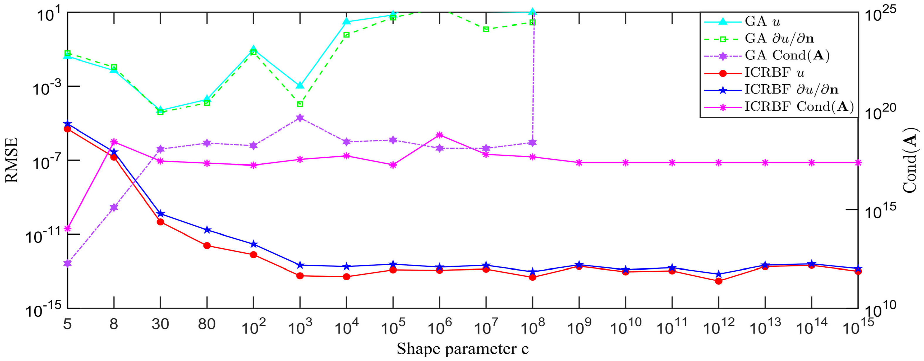
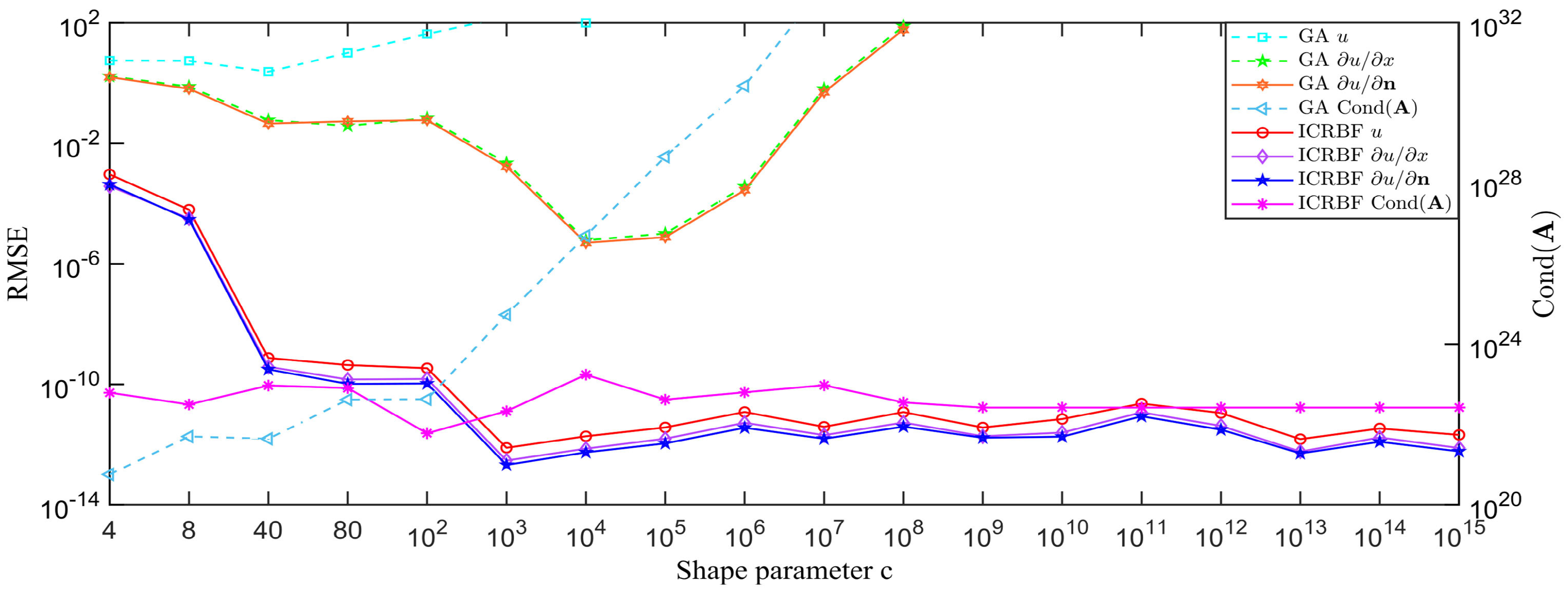
The distribution of nodes is illustrated in Figure 1. First, the optimal value of m is determined using PSO for the case where $\delta =0$. The PSO algorithm determines that $m=3.999999999999775$ is the optimal coupling index. To verify the high efficiency of the ICRBF, we apply the GA + CU ($\epsilon =0.0286$, $\rho ={10}^{-9}$) and GA + CU ($\epsilon =0.0152$, $\rho ={10}^{-11}$) methods in [43] for comparison, where ε is the shape parameter and ρ is the weight.

Table 1. Comparison of relative error of temperature at the point (1.5, 0).

Method	Temperature Value	Error (%)
Exact solution	2.250	0
Onishi, FEM 36 elements [42]	2.323	3.2
Onishi, FEM 144 elements [42]	2.341	4.0
RBF, 49 elements ($c=3$) [11]	2.296	2.0
RBF, 49 elements ($c=4$) [11]	2.251	0.04
GA + CU ($\epsilon =0.0286,\rho ={10}^{-9}$) [43]	2.2501	6.4741 × ${10}^{-3}$
GA + CU ($\epsilon =0.0152,\rho ={10}^{-11}$) [43]	2.2499	2.9952 × ${10}^{-3}$
ICRBF ($\delta =0.01$)	2.2495	0.02170
ICRBF ($\delta =0.001$)	2.2514	0.062391
ICRBF ($\delta =0.0001$)	2.2499	5.2558 × ${10}^{-03}$
ICRBF ($\delta =0.0$)	2.2500	1.6185 × ${10}^{-12}$

lists the temperature solutions recovered at a specific point (1.5, 0) by the above methods, the ICRBF and other methods at different error levels, and the corresponding relative errors. It is clear that, in the absence of noise, the new RBF introduced in this study, which uses the ICRBF as the kernel, achieves significantly higher accuracy compared to other methods. The numerical solutions obtained are superior to those in [11,42] ($c=3$), even when 1% noise perturbation is applied. Figure 2 compares the recovered temperature and temperature flux with the corresponding exact solutions under different noise levels. It is evident that the numerical solutions for both the temperature and flux align well with the analytical solution, even with the addition of a 1% perturbation. Figure 3 shows the condition number $cond\left(\mathbf{A}\right)$ of the numerical matrices and the RMSE of the recovered temperature u and temperature flux $\partial u/\partial \mathbf{n}$ on the unknown boundary obtained using the GA-RBF and ICRBF for various values of c at $\delta =0$ on the unknown boundary. It can be observed that for $c\ge {10}^3$, the introduction of the new kernel of the RBF with the ICRBF results in highly accurate and stable numerical solutions. Moreover, the numerical results are nearly independent of the shape parameter.

Example 2.

Consider an inverse problem of steady-state heat conduction with variable coefficients [29] in a square region containing a rectangular hole. The domain is a unit rectangle $\left\{\right(x,y\left)\right|0\le x\le 1,0\le y\le 1\}$ with an inner rectangular hole $\left\{\right(x,y\left)\right|0.4\le x\le 0.6,0.4\le y\le 0.6\}$. The objective is to evaluate the temperature and flux on the inner boundary ${\mathsf{\Gamma }}_2$ using Cauchy data provided on the outer boundary ${\mathsf{\Gamma }}_1$. The boundary value problem in the computational domain with the hole is described by the following:

$$(2-x^2-y^2)u_{xx}+e^{x+y}{u}_{yy}+2x{u}_x+2y{u}_y+u=f\left(x\right),$$

with the exact solution given by the following:

$$u(x,y)=e^{2x}sin4y+y^3-x^{2}y+sin2x.$$

In the example, we consider two scenarios of noisy data: one is the same as in Example 1, and the other involves random noise:

$$g(x,y)=u(x,y)+\delta rand\left(\right),$$

where $rand\left(\right)$ generates a random number between 0 and 1. In [29], the piecewise smooth radial basis function $r^{11}$ is used as the kernel function. While this approach avoids the need for shape parameters, it achieves only an algebraic convergence rate. In this paper, we introduce the ICRBF as the kernel function to solve the inverse problem of steady-state heat conduction. By coupling an infinitely smooth radial basis function with a piecewise smooth radial basis function, the proposed method inherits the high accuracy of the former and the stability advantages of the latter while eliminating the challenges associated with optimizing shape parameters.

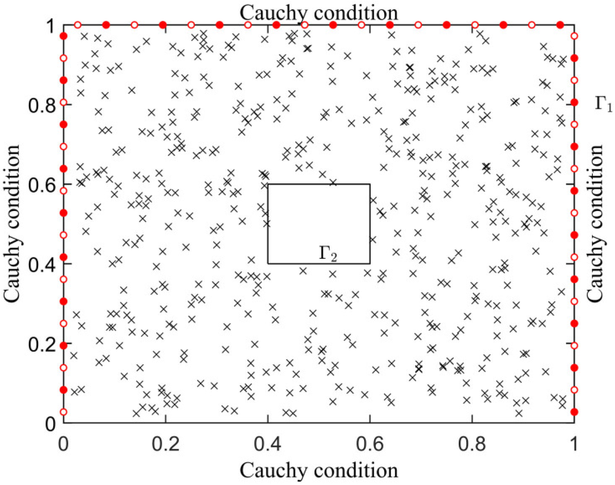
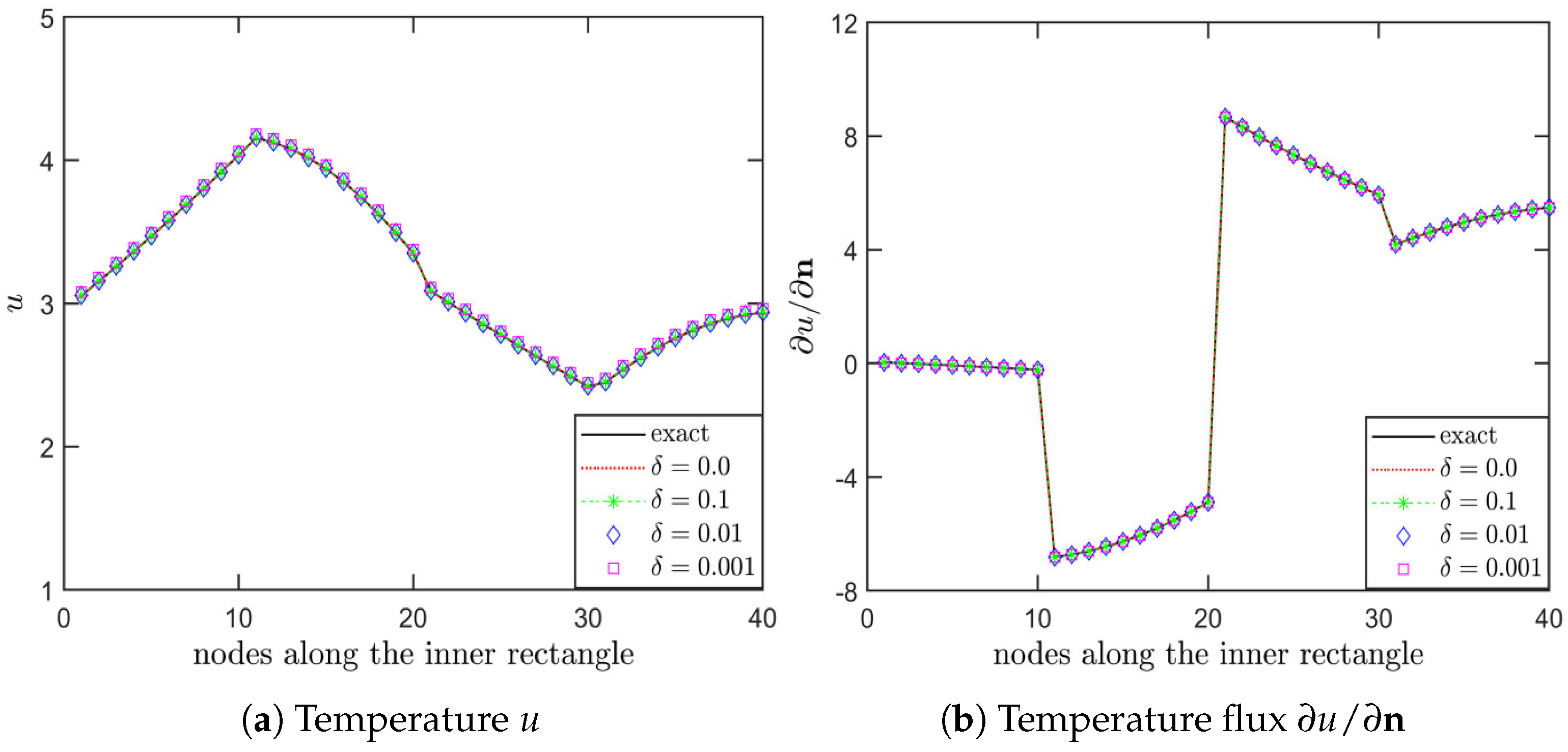
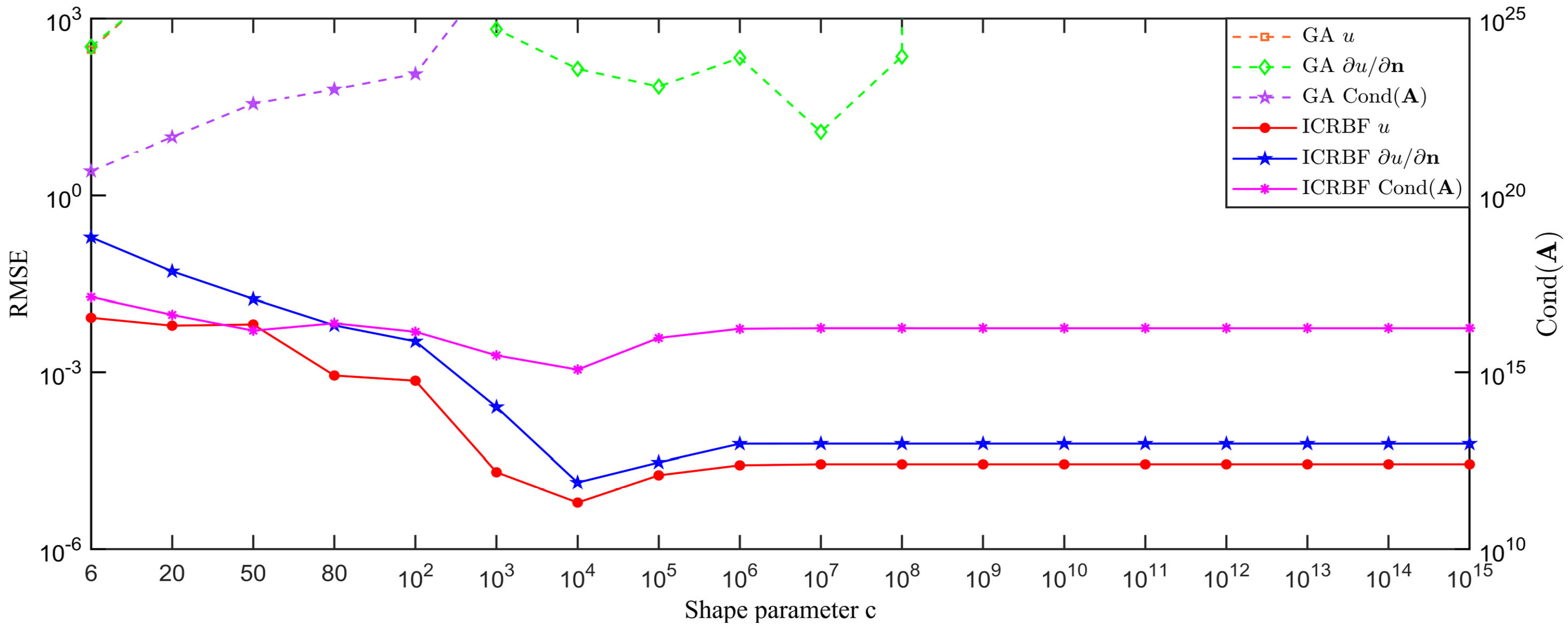
Figure 4 illustrates the distribution of nodes, with 470 randomly distributed configuration nodes for the governing equation. PSO determines the optimal Cindex $m=9.45689235169$ for the case where $\delta =0$. For noise modeled as $\delta sin\left(\pi \right(x+y\left)\right)$, Figure 5 compares the exact values of the temperature and flux with the recovered values under varying noise levels. Additionally, we tested the method with random noise at levels $\delta =0.0,0.1,0.01,0.001$. The results for the temperature and fluxes on the unknown boundary of the inner rectangle are presented in Figure 6. Notably, the recovered temperature and flux using the proposed method align more closely with the exact values at a noise level of $\delta =0.1$ compared to the results at $\delta =0.01$ in [29]. The data in Figure 5 and Figure 6 show that regardless of what form of noise interference is added on the known boundary, the ICRBF can reconstruct an accurate numerical solution. Finally, Figure 7 plots the RMSE and the condition numbers of the numerical matrices for the temperature and flux solutions as functions of the shape parameter c. Three sets of comparison curves show that the ICRBF can obtain accurate numerical solutions and stable condition numbers with a large shape parameter. The ICRBF expands the range of shape parameter values that can effectively obtain accurate solutions.

Example 3.

We investigate the applicability and computational accuracy of the ICRBF method in complex domains. The steady-state heat conduction problem is governed by the following equation [37]:

$$\nabla (\mathbf{D}\nabla u)+f=0,$$

subject to the Dirichlet and Neumann boundary conditions derived from the exact solution:

$$u=x_1^2+x_2^2-5x_1{x}_2,$$

where the parameter $\mathbf{D}$ is expressed as follows:

$$\mathbf{D}=\left[\begin{array}{cc}{(2x_1+x_2+2)}^2& {(x_1-x_2)}^2\\ {(x_1-x_2)}^2& {(x_1+2x_2+2)}^2\end{array}\right].$$

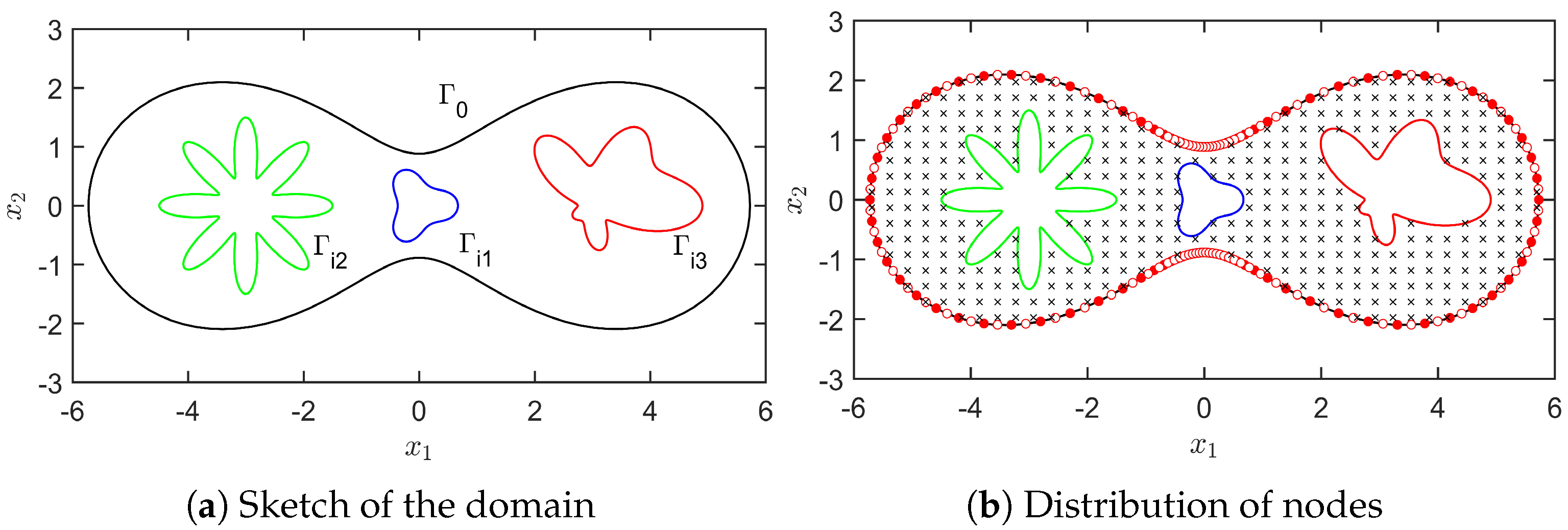
The boundary of the problem is defined as $\mathsf{\Gamma }={\mathsf{\Gamma }}_0+{\mathsf{\Gamma }}_{i1}+{\mathsf{\Gamma }}_{i2}+{\mathsf{\Gamma }}_{i3}$, where for $\theta \in [0,2\pi ]$ the following apply:

$$\begin{array}{cc}\hfill & {\mathsf{\Gamma }}_0=\left\{(x,y)\right|x={\rho }_0\left(\theta \right)cos\theta ,y={\rho }_0\left(\theta \right)sin\theta \},\hfill \\ \hfill & {\mathsf{\Gamma }}_{i1}=\left\{(x,y)\right|x={\rho }_{i1}\left(\theta \right)cos\theta ,y={\rho }_{i1}\left(\theta \right)sin\theta \},\hfill \\ \hfill & {\mathsf{\Gamma }}_{i2}=\left\{(x,y)\right|x=-3+{\rho }_{i2}\left(\theta \right)cos\theta ,y={\rho }_{i2}\left(\theta \right)sin\theta \},\hfill \\ \hfill & {\mathsf{\Gamma }}_{i3}=\left\{(x,y)\right|x=3+{\rho }_{i3}\left(\theta \right)cos\theta ,y={\rho }_{i3}\left(\theta \right)sin\theta \}\hfill \end{array}$$

with

$$\begin{array}{cc}\hfill & {\rho }_0\left(\theta \right)=4\sqrt{cos2\theta +\sqrt{1.1-{sin}^{2}2\theta }},\hfill \\ \hfill & {\rho }_{i1}\left(\theta \right)=0.5{(cos3\theta +\sqrt{2-{sin}^{2}3\theta })}^{1/3},\hfill \\ \hfill & {\rho }_{i2}\left(\theta \right)=0.5+{cos}^{2}4\theta ,\hfill \\ \hfill & {\rho }_{i3}\left(\theta \right)=0.7(e^{sin\theta }{sin}^{2}2\theta +e^{cos\theta }{cos}^{2}2\theta ).\hfill \end{array}$$

The goal is to recover the temperature and fluxes on the inner boundary ${\mathsf{\Gamma }}_2={\mathsf{\Gamma }}_{i1}+{\mathsf{\Gamma }}_{i2}+{\mathsf{\Gamma }}_{i3}$ using Cauchy data provided on the outer boundary ${\mathsf{\Gamma }}_1={\mathsf{\Gamma }}_0$.

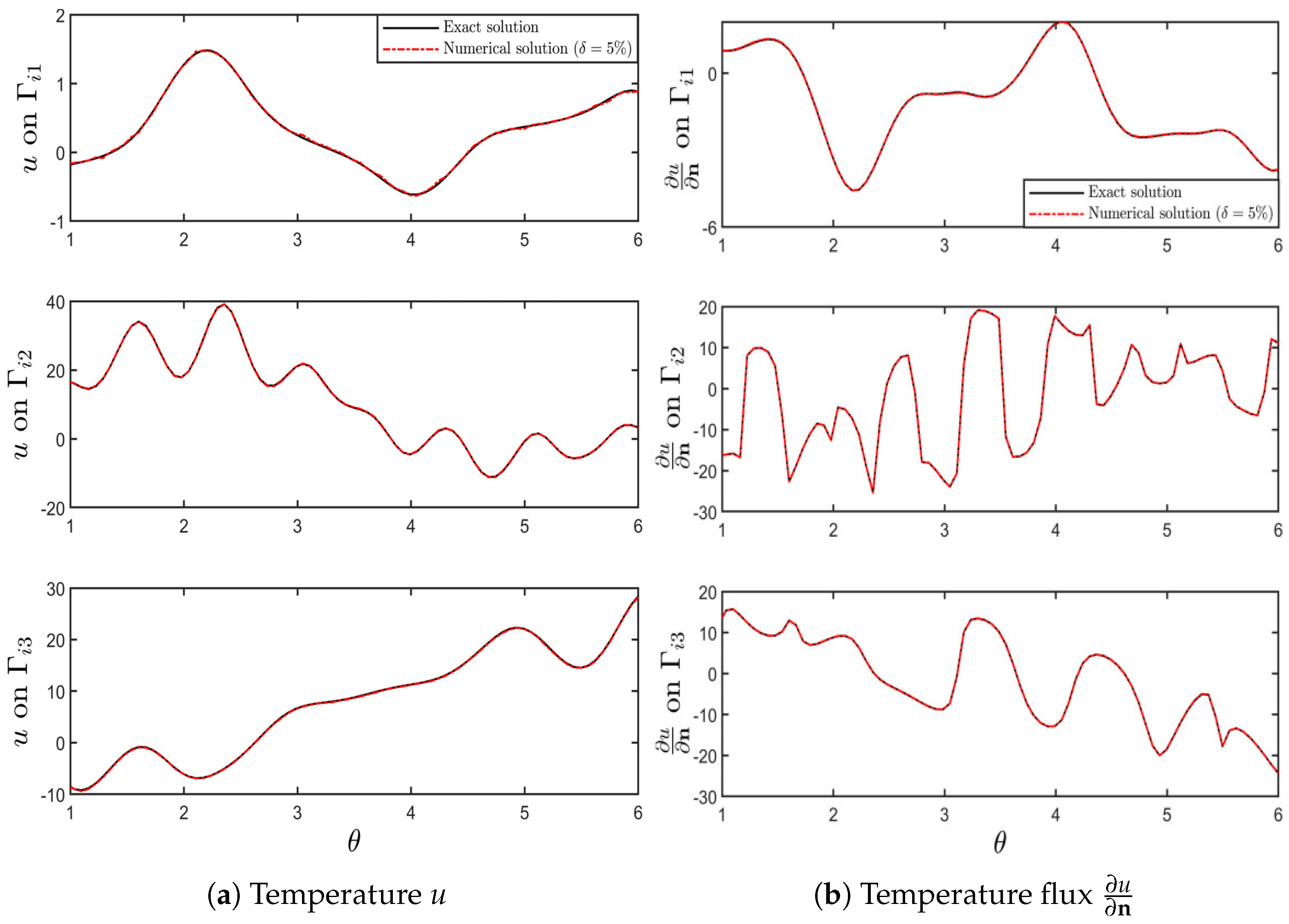
Figure 8 illustrates the problem domain and the distribution of configuration points, which consist of 200 boundary points and 362 internal collocation points. In this test, the optimal Cindex $m=3.999999999999966$ is determined using PSO.

Table 2. The RMSEs of the temperature field on unknown boundaries.

Noise Levels ($\mathit{\delta }$)	${\mathsf{\Gamma }}_{\mathit{i}1}$	${\mathsf{\Gamma }}_{\mathit{i}2}$	${\mathsf{\Gamma }}_{\mathit{i}3}$
0.01%	3.38 × ${10}^{-5}$	1.70 × ${10}^{-4}$	1.85 × ${10}^{-4}$
0.1%	4.42 × ${10}^{-4}$	1.79 × ${10}^{-3}$	2.80 × ${10}^{-3}$
1%	3.10 × ${10}^{-3}$	2.01 × ${10}^{-2}$	1.01 × ${10}^{-2}$

presents the RMSEs of the field temperature on the unknown boundaries under different degrees of random noise interference. As shown in Figure 9, the temperature and flux field solutions obtained using the ICRBF method exhibit excellent agreement with the exact solutions, even at a 5% error level. Table 2 and Figure 9 confirm the stability of the ICRBF. Additionally, Figure 10 demonstrates that the proposed ICRBF method can achieve accurate and stable solutions without being influenced by the shape parameter, provided there is no error interference.

Example 4.

To evaluate the effectiveness of the ICRBF method in high-dimensional scenarios, we apply it to two three-dimensional steady-state heat conduction problems. First, we examine steady-state heat conduction in a unit cube [7], where the left and right faces are treated as unknown boundaries (denoted as ${\mathsf{\Gamma }}_2$), meaning no boundary conditions are specified. The remaining boundaries, referred to as ${\mathsf{\Gamma }}_1$, are over-specified. The temperature and temperature flux on ${\mathsf{\Gamma }}_1$ are used to reconstruct the temperature and flux on the unknown boundary ${\mathsf{\Gamma }}_2$. The governing equation for steady-state heat conduction in this cube is as follows:

$$a(x,y,z)(u_{xx}+u_{yy}+u_{zz})+a_x{u}_x+a_y{u}_y+a_z{u}_z=f\left(x\right),$$

where the coefficient $a(x,y,z)=x^2+y^2+z^2$, and the exact solution is as follows:

$$u(x,y,z)=e^{x}cosy+z.$$

In this problem, an $8\times 8\times 8$ grid of nodes is set up within the domain, and a $7\times 7$ grid of nodes is placed on each face of boundary ${\mathsf{\Gamma }}_1$. The PSO algorithm optimizes the optimal Cindex $m=11.00329568691$. Figure 11 illustrates the field temperature on the left boundary of the cube under random noise interference at various levels. The solid and dotted lines represent the exact solution and the numerical solution obtained using the ICRBF as the kernel function, respectively. It is evident that the temperature recovered by the proposed method aligns more closely with the exact solution as the noise level decreases. Figure 12 displays contour plots of the relative error in temperature at the right boundary under noise perturbation.

Table 3. The AREs for the temperature and the number of interior points ME = n_i × n_i × n_i with 1% noise.

ni	5	6	7	8	9	10
ARE	5.55 × ${10}^{-3}$	3.21 × ${10}^{-3}$	2.82 × ${10}^{-3}$	2.81 × ${10}^{-3}$	3.20 × ${10}^{-3}$	3.37 × ${10}^{-3}$

lists the relative errors of the temperature, which varies slowly with an increasing number of configuration points in the domain, even after applying 1% noise. Figure 11 and Figure 12 and Table 3 demonstrate that the ICRBF-based Kansa method produces highly accurate solutions even in the presence of noise. Finally, Figure 13 depicts the RMSEs of temperature and heat flux at test points under different shape parameters on the unknown boundary, as well as the condition number of the numerical matrix. For the inverse problem of steady-state heat conduction with variable coefficients composed of trigonometric functions in analytical solutions, the traditional GA-RBF cannot obtain accurate numerical solutions, and the ICRBF can not only obtain more accurate numerical solutions but also obtain stable numerical solutions in terms of shape parameters.

Example 5.

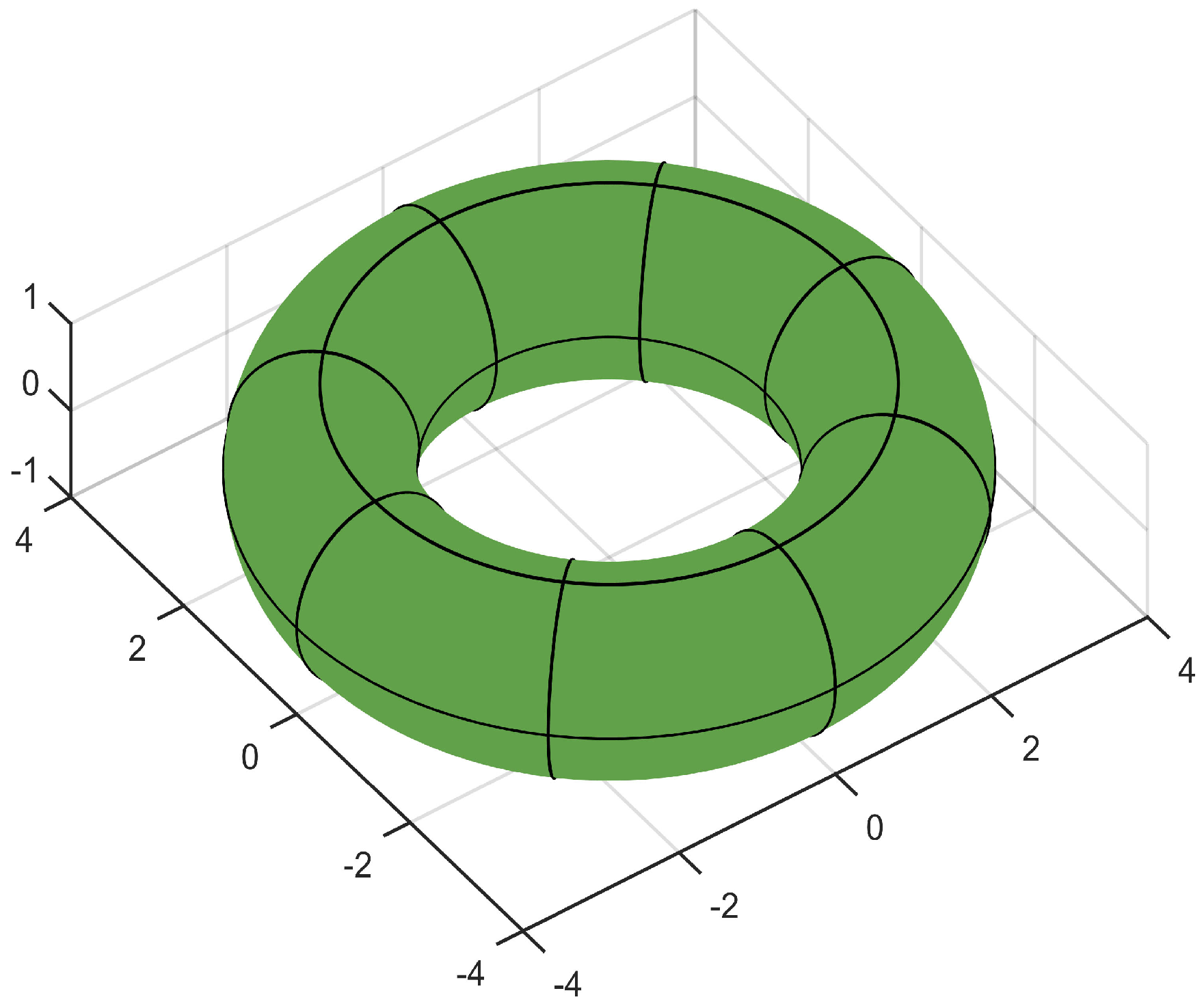
The second three-dimensional example examines the inverse problem of steady-state heat conduction in a ring torus region [38]. The solution domain is a ring torus with radii $R_1=3.0$ and $R_2=1.0$, as shown in Figure 14, defined as follows:

$$\mathsf{\Omega }=\{\mathbf{x}\in {\mathbb{R}}^3|{(\sqrt{x^2+y^2}-R_1)}^2+z^2<R_2^2\}.$$

The governing equation is as follows:

$$\begin{array}{cc}\hfill & y^5{\displaystyle \frac{{\partial }^{2}u}{\partial x^2}}-2xy{\displaystyle \frac{{\partial }^{2}u}{\partial x\partial y}}+(5-2x^3){\displaystyle \frac{{\partial }^{2}u}{\partial y^2}}\hfill \\ \hfill & +(2+z^2){\displaystyle \frac{{\partial }^{2}u}{\partial z^2}}+2x{\displaystyle \frac{\partial u}{\partial x}}+2y{\displaystyle \frac{\partial u}{\partial y}}-2u\hfill \\ \hfill & =6x{y}^5+2x{z}^2+2y^2+4x.\hfill \end{array}$$

The Cauchy boundary condition is derived from the analytical solution:

$$u=x^3+y^2+x{z}^2+5xy+3yz+3x+5.$$

The over-specified boundary ${\mathsf{\Gamma }}_1$ is defined as ${\mathsf{\Gamma }}_1=\{x=(R_1+R_{2}cos\phi )cos\theta ,y=(R_1+R_{2}cos\phi )sin\theta ,$$z=R_{2}sin\phi |0\le \phi \le \pi \}$.

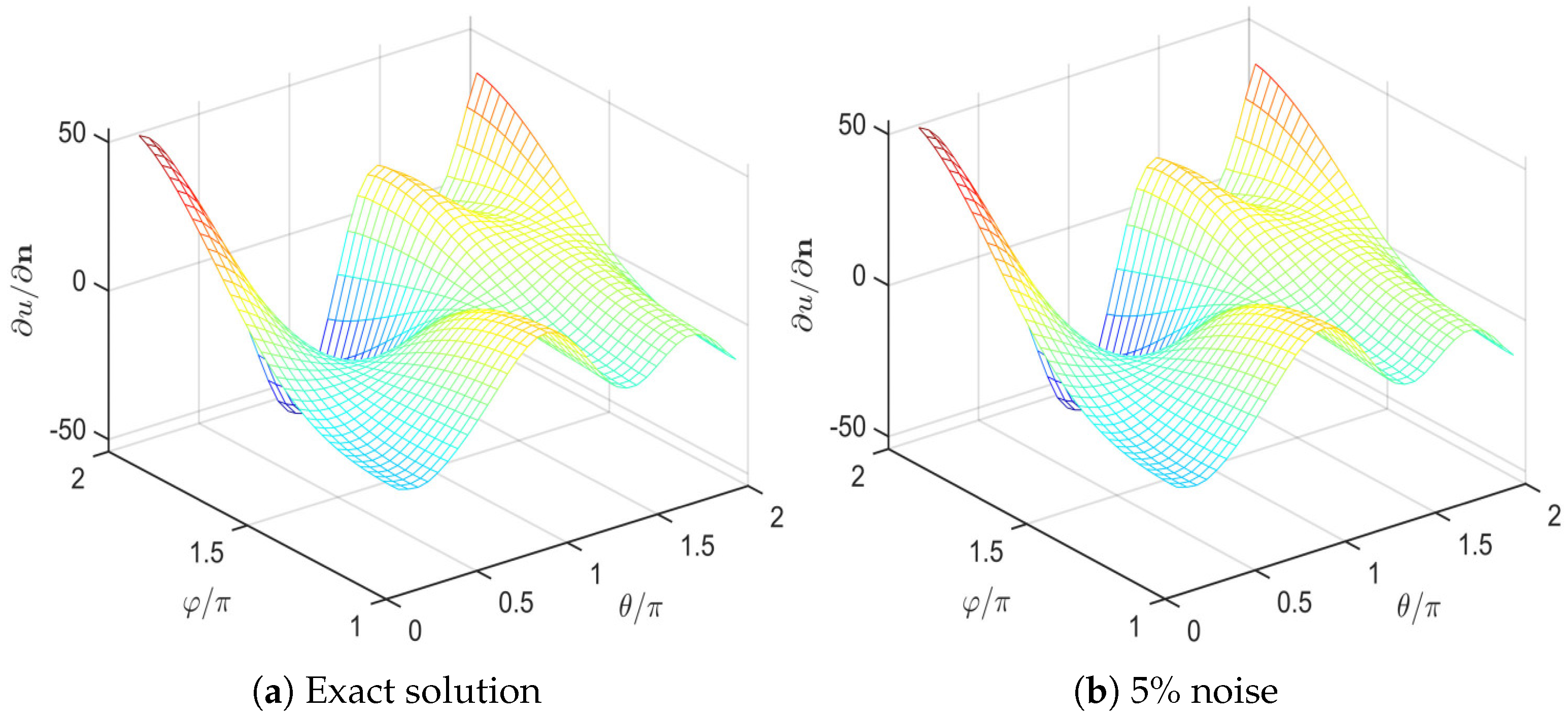
To solve this problem, we use 200 boundary points on the known boundary ${\mathsf{\Gamma }}_1$ and 128 internal configuration points. The internal points are distributed on a grid that divides the cuboid ${[-4,4]}^2\times [-1,1]$ into a $12\times 12\times 4$ grid, ensuring they lie within Ω. The 200 boundary nodes are generated by uniformly partitioning the $\theta \phi$-parameter plane $[0,2\pi ]\times [0,\pi ]$ into $20\times 10$ nodes. The optimal Cindex $m=6.000000000000031$ is determined using PSO. Figure 15 and Figure 16 compare the exact solution with the recovered analytical solution for the temperature and heat fluxes on the unknown boundary after applying a 5% random error noise perturbation. This confirms that even under high levels of noise interference, the ICRBF can obtain a numerical solution close to the exact solution. With the same number of boundary points and interior points, and the same distribution of the configuration points, we apply the method in [38] to filter out the integer-valued Cindex $m=6$, and we abbreviate the kernel function at this Cindex as $CG{A}_{m6}$. We compare the temperature and heat flux solutions recovered from the $CG{A}_{m6}$ with the ICRBF for the real-valued Cindex at different error levels, as shown in

Table 4. RMSEs of numerical solutions under different noise levels.

$\mathit{\delta }$	${\mathbf{CGA}}_{\mathit{m}6}$		ICRBF
	Temperature $\mathit{u}$	Heat Flux $\partial \mathit{u}/\partial \mathit{n}$	Temperature $\mathit{u}$	Heat Flux $\partial \mathit{u}/\partial \mathit{n}$
0	1.18 × ${10}^{-7}$	1.37 × ${10}^{-7}$	4.63 × ${10}^{-8}$	5.99 × ${10}^{-8}$
1%	4.04 × ${10}^{-2}$	3.69 × ${10}^{-2}$	4.03 × ${10}^{-3}$	4.82 × ${10}^{-3}$
3%	7.54 × ${10}^{-2}$	1.05 × ${10}^{-2}$	1.37 × ${10}^{-2}$	1.58 × ${10}^{-2}$
5%	1.60 × ${10}^{-1}$	1.66 × ${10}^{-1}$	2.24 × ${10}^{-2}$	2.61 × ${10}^{-2}$

. The ICRBF obtains more accurate numerical solutions for the same shape parameter $c=1000$ as well as noise interferences. Figure 17 shows the variation curves of the RMSEs for the reconstructed temperature solution u; the heat flux solution $\partial u/\partial \mathbf{n}$; and the condition number of the numerical matrix for the conventional GA-RBF, $CG{A}_{m6}$-RBF, and ICRBF as functions of the shape parameters. It can be seen that although $m=6.000000000000031$ is very close to 6, the numerical solutions obtained by the ICRBF for some shape parameters are a little more accurate and stable. These results demonstrate that the shape parameter has minimal impact on the accuracy and stability of the method in solving the three-dimensional inverse problem of steady-state heat conduction.

5. Conclusions

This study proposes a novel ICRBF method through the coupling of the GA and conical spline of the optimized Cindex. The primary innovation lies in employing PSO to extend the Cindex from integer to real-number domains, significantly enhancing parameter selection flexibility. For the first time, this approach is applied to solve variable-coefficient steady-state heat conduction Cauchy inverse problems. Compared with the existing methods for solving the Cauchy inverse of heat conduction problem, the ICRBF does not need to regularize the numerical matrix and can directly solve the inverse problem.

The numerical results indicate that when the coupling index is a real number, the ICRBF can still achieve an accurate numerical solution even in the presence of noise disturbances on the known boundary. Furthermore, the ICRBF broadens the range of values for the shape parameter; it remains capable of delivering precise numerical solutions and maintaining a reasonable condition number, even with large shape parameters.

In addition to addressing the steady-state heat conduction inverse problem discussed in this study, the ICRBF can be extended to tackle problems related to the Helmholtz equation, elasticity problems, and transient problems. Notably, when applied to high-dimensional problems, the ICRBF continues to yield satisfactory numerical solutions. The ICRBF has several advantages, including simplicity, meshless implementation, high computational accuracy, numerical stability, and applicability to high-dimensional and variable coefficient problems.

References

1. Colton, D.; Kress, R. Inverse Acoustic and Electromagnetic Scattering Theory; Springer: New York, NY, USA, 1998; pp. 195–206. [Google Scholar]
2. Balaban, A.; Grechikhin, V.; Yufanova, J. Inverse problems in the design of electromagnetic mechanisms of ground vehicle magnetic levitation systems. Transp. Res. Procedia 2022, 63, 1171–1179. [Google Scholar] [CrossRef]
3. Laves, M.H.; Tölle, M.; Schlaefer, A.; Engelhardt, S. Posterior temperature optimized Bayesian models for inverse problems in medical imaging. Med. Image Anal. 2022, 78, 102382. [Google Scholar] [CrossRef] [PubMed]
4. Ali, A.; Al-Mamun, A.; Pereira, F.; Rahunanthan, A. Multiscale sampling for the inverse modeling of partial differential equations. J. Comput. Phys. 2024, 497, 112609. [Google Scholar] [CrossRef]
5. Fu, Z.J.; Chen, W.; Zhang, C.Z. Boundary particle method for Cauchy inhomogeneous potential problems. Inverse Probl. Sci. Eng. 2012, 20, 189–207. [Google Scholar] [CrossRef]
6. Li, Y.X.; Hu, X.L. Artificial neural network approximations of Cauchy inverse problem for linear PDEs. Appl. Math. Comput. 2022, 414, 126678. [Google Scholar] [CrossRef]
7. Hu, W.; Fu, Z.J.; Tang, Z.C.; Gu, Y. A meshless collocation method for solving the inverse Cauchy problem associated with the variable-order fractional heat conduction model under functionally graded materials. Eng. Anal. Bound. Elem. 2022, 140, 132–144. [Google Scholar] [CrossRef]
8. Nguyen, A.T.; Tuan, N.H.; Yang, C. On Cauchy problem for fractional parabolic-elliptic Keller-Segel model. Adv. Nonlinear Anal. 2023, 12, 97–116. [Google Scholar] [CrossRef]
9. Aronson, D.G.; Besala, P. Uniqueness of solutions of the Cauchy problem for parabolic equations. J. Math. Anal. Appl. 1966, 13, 516–526. [Google Scholar] [CrossRef]
10. Chakib, A.; Nachaoui, A. Convergence analysis for finite element approximation to an inverse Cauchy problem. Inverse Probl. 2006, 22, 1191–1206. [Google Scholar] [CrossRef]
11. Cheng, A.H.D.; Cabral, J.J.S.P. Direct solution of ill-posed boundary value problems by radial basis function collocation method. Int. J. Numer. Methods Eng. 2005, 64, 45–64. [Google Scholar] [CrossRef]
12. Ly, I. An iterative method for solving Cauchy problems for the p-Laplace operator. Complex Var. Elliptic Equ. 2010, 55, 1079–1088. [Google Scholar] [CrossRef]
13. Wang, F.J.; Fan, C.M.; Hua, Q.S.; Gu, Y. Localized MFS for the inverse Cauchy problems of two-dimensional Laplace and biharmonic equations. Appl. Math. Comput. 2020, 364, 124658. [Google Scholar] [CrossRef]
14. Gong, R.F.; Wang, M.; Huang, Q.; Zhang, Y. A CCBM-based generalized GKB iterative regularization algorithm for inverse Cauchy problems. J. Comput. Appl. Math. 2023, 432, 115282. [Google Scholar] [CrossRef]
15. Hu, X.Z.; Mu, L.; Ye, X. A simple finite element method of the Cauchy problem for Poisson equation. Int. J. Numer. Anal. Model. 2017, 14, 591–603. [Google Scholar]
16. Bakushinsky, B.A.; Kokurin, Y.M.; Kokurin, M.M. On a class of finite difference methods for ill-posed Cauchy problems with noisy data. J. Inverse Ill-Posed Probl. 2011, 18, 959–977. [Google Scholar] [CrossRef]
17. Ellabib, A.; Nachaoui, A.; Ousaadane, A. Mathematical analysis and simulation of fixed point formulation of Cauchy problem in linear elasticity. Math. Comput. Simul. 2021, 187, 231–247. [Google Scholar] [CrossRef]
18. Li, W.; Liu, X.Y.; Yao, G.M. A local meshless collocation method for solving certain inverse problems. Eng. Anal. Bound. Elem. 2015, 57, 9–15. [Google Scholar] [CrossRef]
19. Safari, F. Solving multi-dimensional inverse heat problems via an accurate RBF-based meshless technique. Int. J. Heat Mass Transf. 2023, 209, 124100. [Google Scholar] [CrossRef]
20. Lamm, P.K. Future-sequential regularization methods for III-posed Volterra equations: Applications to the inverse heat conduction problem. J. Math. Anal. Appl. 1995, 195, 469–494. [Google Scholar] [CrossRef]
21. Dreglea, A.; Sidorov, N. Integral equations in identification of external force and heat source density dynamics. Bull. Acad. Științe Repub. Mold. Mat. 2018, 88, 68–77. [Google Scholar]
22. Dardé, J.; Hannukainen, A.; Hyvönen, N. An hdiv-based mixed quasi-reversibility method for solving elliptic Cauchy problems. SIAM J. Numer. Anal. 2013, 51, 2123–2148. [Google Scholar] [CrossRef]
23. Chen, C.S.; Amuzu, L.; Acheampong, K.; Zhu, H. Improved geometric modeling using the method of fundamental solutions. Eng. Anal. Bound. Elem. 2021, 130, 49–57. [Google Scholar] [CrossRef]
24. Fu, Z.J.; Chen, W.; Qin, Q.H. Boundary knot method for heat conduction in nonlinear functionally graded material. Eng. Anal. Bound. Elem. 2011, 35, 729–734. [Google Scholar] [CrossRef]
25. Zhang, Y.M.; Sun, F.L.; Qu, W.Z.; Gu, Y.; Young, D.L. A meshless average source boundary node method for steady-state heat conduction in general anisotropic media. Comput. Math. Appl. 2018, 75, 1739–1755. [Google Scholar] [CrossRef]
26. Kovářík, K.; Mužík, J.; Gago, F.; Sitányiová, D. Modified local singular boundary method for solution of two-dimensional diffusion equation. Eng. Anal. Bound. Elem. 2022, 143, 525–534. [Google Scholar] [CrossRef]
27. Fu, Z.J.; Yang, L.W.; Xi, Q.; Liu, C.S. A boundary collocation method for anomalous heat conduction analysis in functionally graded materials. Comput. Math. Appl. 2021, 88, 91–109. [Google Scholar] [CrossRef]
28. Borkowska, D.; Borkowski, M. A numerical analysis of the generalised collocation Trefftz method for some 2D Laplace problems. Eng. Anal. Bound. Elem. 2023, 152, 608–626. [Google Scholar] [CrossRef]
29. Li, J.C. A radial basis meshless method for solving inverse boundary value problems. Commun. Numer. Methods Eng. 2003, 20, 51–61. [Google Scholar] [CrossRef]
30. Liu, C.S.; Chen, W.; Fu, Z.J. A multiple-scale MQ-RBF for solving the inverse Cauchy problems in arbitrary plane domain. Eng. Anal. Bound. Elem. 2016, 68, 11–16. [Google Scholar] [CrossRef]
31. Chen, Y.T.; Li, C.; Yao, L.Q.; Cao, Y. A hybrid RBF collocation method and its application in the elastostatic symmetric problems. Symmetry 2022, 14, 1476. [Google Scholar] [CrossRef]
32. Mostajeran, F.; Hosseini, S.M. Radial basis function neural network (RBFNN) approximation of Cauchy inverse problems of the Laplace equation. Comput. Math. Appl. 2023, 141, 129–144. [Google Scholar] [CrossRef]
33. Cheng, A.H.-D. Multiquadric and its shape parameter-a numerical investigation of error estimate, condition number, and round-offerror by arbitrary precision computation. Eng. Anal. Bound. Elem. 2012, 36, 220–239. [Google Scholar] [CrossRef]
34. Chen, W.; Hong, Y.; Lin, J. The sample solution approach for determination of the optimal shape parameter in the multiquadric function of the Kansa method. Comput. Math. Appl. 2018, 75, 2942–2954. [Google Scholar] [CrossRef]
35. Wang, F.; Chen, W.; Zhang, C.; Hua, Q. Kansa method based on the Hausdorff fractal distance for Hausdorff derivative Poisson equations. Fractals 2018, 26, 1850084. [Google Scholar] [CrossRef]
36. Liu, C.-S.; Liu, D. Optimal shape parameter in the MQ-RBF by minimizing an energy gap functional. Appl. Math. Lett. 2018, 86, 157–165. [Google Scholar] [CrossRef]
37. Zhang, Y.M. An accurate and stable RBF method for solving partial differential equations. Appl. Math. Lett. 2019, 97, 93–98. [Google Scholar] [CrossRef]
38. Zhang, C.; Fu, Z.J.; Zhang, Y.M. A novel global RBF direct collocation method for solving partial differential equations with variable coefficients. Eng. Anal. Bound. Elem. 2024, 160, 14–27. [Google Scholar] [CrossRef]
39. Eberhart, R.C.; Kennedy, J. A new optimizer using particle swarm theory. In Proceedings of the 6th International Symposium on Micro Machine and Human Science, Nagoya, Japan, 4–6 October 1995; pp. 39–43. [Google Scholar]
40. Fasshauer, G.E.; Zhang, J.G. On choosing optimal shape parameters for RBF approximation. Numer. Algorithms 2007, 45, 345–368. [Google Scholar] [CrossRef]
41. Rippa, S. An algorithm for selecting a good value for the parameter c in radial basis function interpolation. Adv. Comput. Math. 1999, 11, 193–210. [Google Scholar] [CrossRef]
42. Onishi, K. Boundary inverse problems in seepage and viscous fluid flows. In Proceedings of the Computer Methods and Water Resources III, Chalkis, Greece, 26–28 September 1995; pp. 457–468. [Google Scholar]
43. Moazami, D.; Esmaeilbeigi, M. Enhanced stability and accuracy in solving nonlinear fredholm integral equations using hybrid radial kernels and particle swarm optimization. Comput. Appl. Math. 2025, 44, 78. [Google Scholar] [CrossRef]
Figure 1. Boundary conditions and distribution of nodes.
Mathematics 13 01423 g001
Figure 2. Comparison of ICRBF solutions and exact solutions on the unknown boundary.
Mathematics 13 01423 g002
Figure 3. The RMSEs of the numerical results and condition number versus the value of c ( δ = 0 ).
Mathematics 13 01423 g003
Figure 4. Boundary conditions and distribution of nodes.
Mathematics 13 01423 g004
Figure 5. Comparison of the ICRBF solutions and exact solutions on the unknown boundary ( δ sin ( π ( x + y ) ) ) .
Mathematics 13 01423 g005
Figure 6. Comparison of the ICRBF solutions and exact solutions on the unknown boundary ( δ r a n d ( ) ) .
Mathematics 13 01423 g006
Figure 7. The RMSEs of the numerical results and condition number versus the value of c ( δ = 0 ).
Mathematics 13 01423 g007
Figure 8. Problem domain and computational model description.
Mathematics 13 01423 g008
Figure 9. Numerical results for temperature u and temperature flux u n on the under-specified surface by using the suggested ICRBF at 5% noise level.
Mathematics 13 01423 g009
Figure 10. The RMSEs of the numerical results and condition number versus the value of c ( δ = 0 ).
Mathematics 13 01423 g010
Figure 11. The distribution of the temperature field at the left unknown boundary with various levels of data noise.
Mathematics 13 01423 g011aMathematics 13 01423 g011b
Figure 12. The distribution of the relative error of the temperature field at the right unknown boundary with various levels of data noise.
Mathematics 13 01423 g012
Figure 13. The RMSEs of the numerical results and condition number versus the value of c (δ = 0).
Mathematics 13 01423 g013
Figure 14. The problem sketch of the ring torus.
Mathematics 13 01423 g014
Figure 15. Surfaces of analytical solutions (a) and profiles of numerical solutions (b) for the temperature field with 5% noise.
Mathematics 13 01423 g015
Figure 16. Surfaces of analytical solutions (a) and profiles of numerical solutions (b) for the temperature flux with 5% noise.
Mathematics 13 01423 g016
Figure 17. The RMSEs of the numerical results and condition number versus the value of c ( δ = 0 ).
Mathematics 13 01423 g017