Exact Solution of Ambartsumian Delay Differential Equation and Comparison with Daftardar-Gejji and Jafari Approximate Method

Abstract

The Ambartsumian equation, a linear differential equation involving a proportional delay term, is used in the theory of surface brightness in the Milky Way. In this paper, the Laplace-transform was first applied to this equation, and then the decomposition method was implemented to establish a closed-form solution. The present closed-form solution is reported for the first time for the Ambartsumian equation. Numerically, the calculations have demonstrated a rapid rate of convergence of the obtained approximate solutions, which are displayed in several graphs. It has also been shown that only a few terms of the new approximate solution were sufficient to achieve extremely accurate numerical results. Furthermore, comparisons of the present results with the existing methods in the literature were introduced.

1. Introduction

In this paper, we consider the Ambartsumian equation [1,2], given by

$$y^{\prime }(t)=-y(t)+\frac{1}{q}y\left(\frac{t}{q}\right),q>1,$$

(1)

where $q$ is a constant for the given model and Equation (1) is subjected to the initial condition:

$$y(0)=\lambda ,$$

(2)

where $\lambda$ is also a constant. It is interesting to mention that Equation (1) (with $q>1$) was derived more than 25 years earlier by Ambartsumian [1] to describe the absorption of light by the interstellar matter. Its existence and uniqueness have been proved and discussed by Kato and McLeod [3]. It is of great importance to search for accurate solutions to Equations (1) and (2) due to their application in Astronomy. Very recently, Patade and Bhalekar [2] obtained a power series solution for this system by applying the Daftardar-Gejji and Jafari Method [4]. They proved the convergence for all $\left|q\right|>1$, however, their solution is not valid in the whole domain as will be shown in this paper. In order to overcome such difficulties, in this paper, a new exact solution was derived using the Laplace-transform and Adomian decomposition method (ADM).

The ADM was applied to solving algebraic/transcendental/matrix equations [5,6,7,8,9], nonlinear integral/differential equations and both of initial and boundary value problems (IVPs/BVPs), even for irregular boundary contours [10,11,12,13,14,15,16,17,18,19,20,21,22,23,24]. The solution for this method is an infinite series, which converges when choosing an appropriate canonical form. Hence, a few terms achieve good accuracy for the model under consideration. This paper considers the idea of obtaining the exact solution of a delay differential equation via the Laplace-transform and ADM. This methodit is not similar to work in Reference [12] or other published works, hence, the present techniques are new. In addition, theoretical analysis for the convergence of Adomian’s method to differential equations has been discussed earlier by Abbaoui and Cherruault [25]. We remark that a significant advantage of the ADM in solving differential equations is that it neither invokes the fixed-point theorem to prove convergence, nor is the Adomian solution algorithm developed under this premise. The speed of convergence and the general error estimation of the series solution using the standard ADM have been previously reported by Cherruault and Adomian [26]. Moreover, Rach [27] introduced an extensive bibliography of the theory, technique, and applications of the Adomian decomposition method.

The objective of this work was to reinvestigate the Ambartsumian delay equation by applying both of the Laplace-transform and the ADM. The obtained analytic closed-form solution can be viewed as a new type of solution for the current problem. It will also be numerically demonstrated that the sequence of the approximate solutions converge faster than the one in the literature [2]. Furthermore, comparisons of the present exact results with those approximately obtained in Reference [2] by using the Daftarday-Gejji and Jafari technique, and [28] by using the homotopy analysis transform method (HATM) will be introduced.

2. Application of the Laplace-Transform and Decomposition Method

Applying Laplace-transform on Equation (1), yields

$$sY(s)-\lambda =-Y(s)+Y(qs),$$

(3)

where $Y(s)$ is the Laplace-transform of $y(t)$ and $Y(qs)$ is the Laplace-transform of $\left(\frac{1}{q}y\left(\frac{t}{q}\right)\right)$. In order to apply the ADM, we rewrite Equation (3) in the following canonical form:

$$Y(s)=\frac{\lambda }{s+1}+\frac{Y(qs)}{s+1}.$$

(4)

Now, we search for a series solution of Equation (4), which leads to a closed-form. The ADM was applied here to achieve this task. It is well-known that the ADM assumes the solution $Y(s)$ as

$$Y(s)={\displaystyle \sum _{i=0}^{\infty }}{Y}_i(s).$$

(5)

On inserting Equation (5) into Equation (4), we then get

$${\displaystyle \sum _{i=0}^{\infty }}{Y}_i(s)=\frac{\lambda }{s+1}+\frac{1}{s+1}{\displaystyle \sum _{i=0}^{\infty }}{Y}_i(qs),$$

(6)

and hence, the following recurrence scheme is established [12,25,26,27]:

$$\begin{array}{l}{Y}_0(s)=\frac{\lambda }{s+1},\\ Y_i(s)=\frac{Y_{i-1}(qs)}{s+1},i\ge 1.\end{array}$$

(7)

The recurrence scheme in Equation (7) was implemented here to obtain a general form of the $Y_i(s)$-component ($i>1$). From Equation (7) at $i=1$, we have

$$\begin{array}{ll}{Y}_1(s)& =\frac{Y_0(qs)}{s+1},\\ & =\frac{\lambda }{(s+1)(qs+1)},\\ & =\frac{\lambda }{{\displaystyle \prod _{k=0}^1}\left(q^{k}s+1\right)}.\end{array}$$

(8)

At $i=2$, we obtain

$$\begin{array}{ll}{Y}_2(s)& =\frac{\lambda }{(s+1)(qs+1)(q^{2}s+1)},\\ & =\frac{\lambda }{{\displaystyle \prod _{k=0}^2}\left(q^{k}s+1\right)}.\end{array}$$

(9)

Similarly, $Y_3(s)$ and $Y_4(s)$ were obtained, respectively, as

$$\begin{array}{ll}{Y}_3(s)& =\frac{\lambda }{(s+1)(qs+1)(q^{2}s+1)(q^{3}s+1)},\\ & =\frac{\lambda }{{\displaystyle \prod _{k=0}^3}\left(q^{k}s+1\right)},\end{array}$$

(10)

and

$$\begin{array}{ll}{Y}_4(s)& =\frac{\lambda }{(s+1)(qs+1)(q^{2}s+1)(q^{3}s+1)(q^{4}s+1)},\\ & =\frac{\lambda }{{\displaystyle \prod _{k=0}^4}\left(q^{k}s+1\right)}.\end{array}$$

(11)

Therefore, the general term $Y_i(s)$ is given by

$$\begin{array}{ll}{Y}_i(s)& =\frac{\lambda }{(s+1)(qs+1)(q^{2}s+1)\dots \dots (q^{i}s+1)},\\ & =\frac{\lambda }{{\displaystyle \prod _{k=0}^i}\left(q^{k}s+1\right)}.\end{array}$$

(12)

Hence, the solution of the transformed Equation (5) is obtained by

$$Y(s)={\displaystyle \sum _{i=0}^{\infty }}\frac{\lambda }{{\displaystyle \prod _{k=0}^i}\left(q^{k}s+1\right)}.$$

(13)

On applying the inverse Laplace transform to Equation (13), we obtain

$$\begin{array}{ll}y(t)& =\lambda {\displaystyle \sum _{i=0}^{\infty }}{L}^{-1}\left[\frac{1}{{\displaystyle \prod _{k=0}^i}\left(q^{k}s+1\right)}\right],\\ & =\lambda {\displaystyle \sum _{i=0}^{\infty }}{L}^{-1}\left[\frac{P(s)}{Q_i(s)}\right],\end{array}$$

(14)

where the two polynomials $P(s)$ (a constant polynomial) and $Q_i(s)$ (a polynomial of degree $(i+1)$ in $s$) are defined by

$$P(s)=1,Q_i(s)={\displaystyle \prod _{k=0}^i}\left(q^{k}s+1\right).$$

(15)

Here, it is important to note that $Q_i(s)$ is a polynomial with distinct $(i+1)$ zeros. In order to calculate the inverse Laplace transform in Equation (14), we used the Heaviside’s expansion formula ([29], p. 46):

$$L^{-1}\left[\frac{P(s)}{Q_i(s)}\right]={\displaystyle \sum _{k=0}^i}\frac{P({\alpha }_k)}{Q_i^{\prime }({\alpha }_k)}\times e^{{\alpha }_{k}t},$$

(16)

where ${\alpha }_k=-q^{-k},(k=0,1,2,\dots i)$ are the distinct zeros of the algebraic equation $Q_i(s)=0$, hence, Equation (16) becomes

$$L^{-1}\left[\frac{P(s)}{Q_i(s)}\right]={\displaystyle \sum _{k=0}^i}\frac{e^{-q^{-k}t}}{Q_i^{\prime }(-q^{-k})}.$$

(17)

Therefore, the closed form solution for Equation (14) is finally written as

$$y(t)=\lambda {\displaystyle \sum _{i=0}^{\infty }}{\displaystyle \sum _{k=0}^i}\frac{e^{-q^{-k}t}}{Q_i^{\prime }(-q^{-k})}.$$

(18)

The $n$-term approximate solution is given by

$${\mathrm{\Phi }}_n(t)=\lambda {\displaystyle \sum _{i=0}^{n-1}}{\displaystyle \sum _{k=0}^i}\frac{e^{-q^{-k}t}}{Q_i^{\prime }(-q^{-k})}.$$

(19)

It can be easily checked that the $n$-term approximate solution for Equation (19) satisfies the initial condition ${\mathrm{\Phi }}_n(0)=\lambda ,\forall n\ge 1$. At $t=0$, Equation (19) becomes

$${\mathrm{\Phi }}_n(0)=\lambda {\displaystyle \sum _{i=0}^{n-1}}{\displaystyle \sum _{k=0}^i}\frac{1}{Q_i^{\prime }(-q^{-k})}.$$

(20)

For illustration, we took $n=2$ as an example and it will be shown that ${\mathrm{\Phi }}_2(0)=\lambda$. Implementing (20) at $n=2$ leads to

$${\mathrm{\Phi }}_2(0)=\lambda {\displaystyle \sum _{i=0}^1}{\displaystyle \sum _{k=0}^i}\frac{1}{Q_i^{\prime }(-q^{-k})},$$

(21)

$$=\lambda \left({\displaystyle \sum _{k=0}^0}\frac{1}{Q_0^{\prime }(-q^{-k})}+{\displaystyle \sum _{k=0}^1}\frac{1}{Q_1^{\prime }(-q^{-k})}\right),$$

(22)

$$=\lambda \left(\frac{1}{Q_0^{\prime }(-1)}+\frac{1}{Q_1^{\prime }(-1)}+\frac{1}{Q_1^{\prime }(-q^{-1})}\right).$$

(23)

The values of $Q_0^{\prime }(-1)$, $Q_1^{\prime }(-1)$, and $Q_1^{\prime }(-q^{-1})$ can be calculated from Equation (15) as follows:

$$Q_0(s)=s+1,Q_1(s)=q{s}^2+(q+1)s+1,$$

(24)

$$Q_0^{\prime }(s)=1,Q_1^{\prime }(s)=2qs+(q+1),$$

(25)

$$Q_0^{\prime }(-1)=1,Q_1^{\prime }(-1)=-q+1,$$

(26)

Subsitituting Equation (26) into Equation (23), we have

$${\mathrm{\Phi }}_2(0)=\lambda \left(1+\frac{1}{-q+1}+\frac{1}{q-1}\right),$$

(27)

$$=\lambda .$$

(28)

In this section, the Laplace transform and the ADM were applied to obtain the closed form solution for Equation (19) for the Ambartsumian equation. The obtained approximate solutions are investigated in the next section to stand on their domains of applicability and validity.

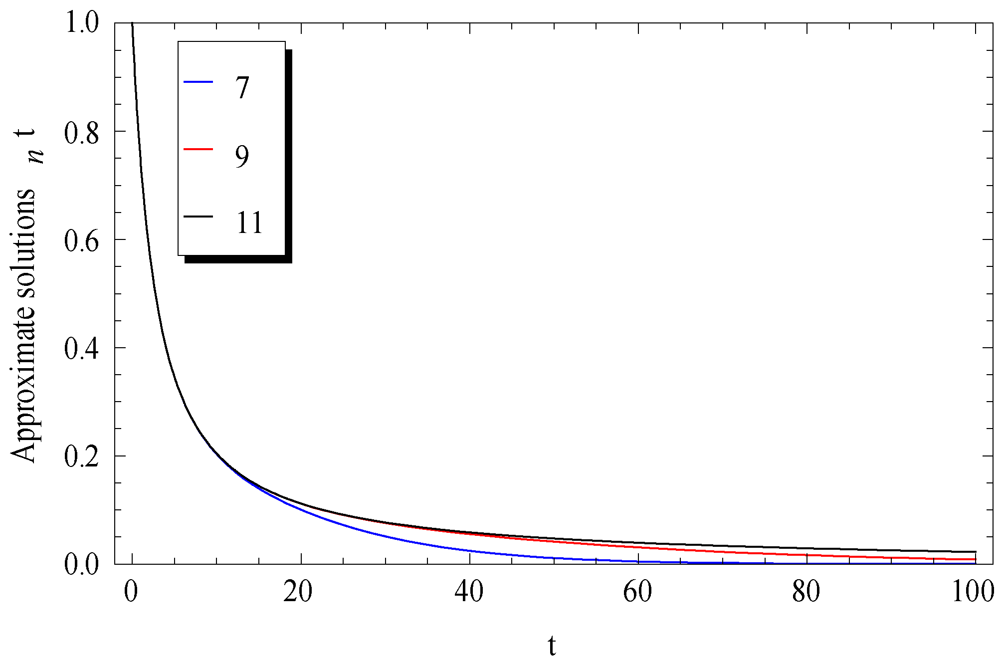
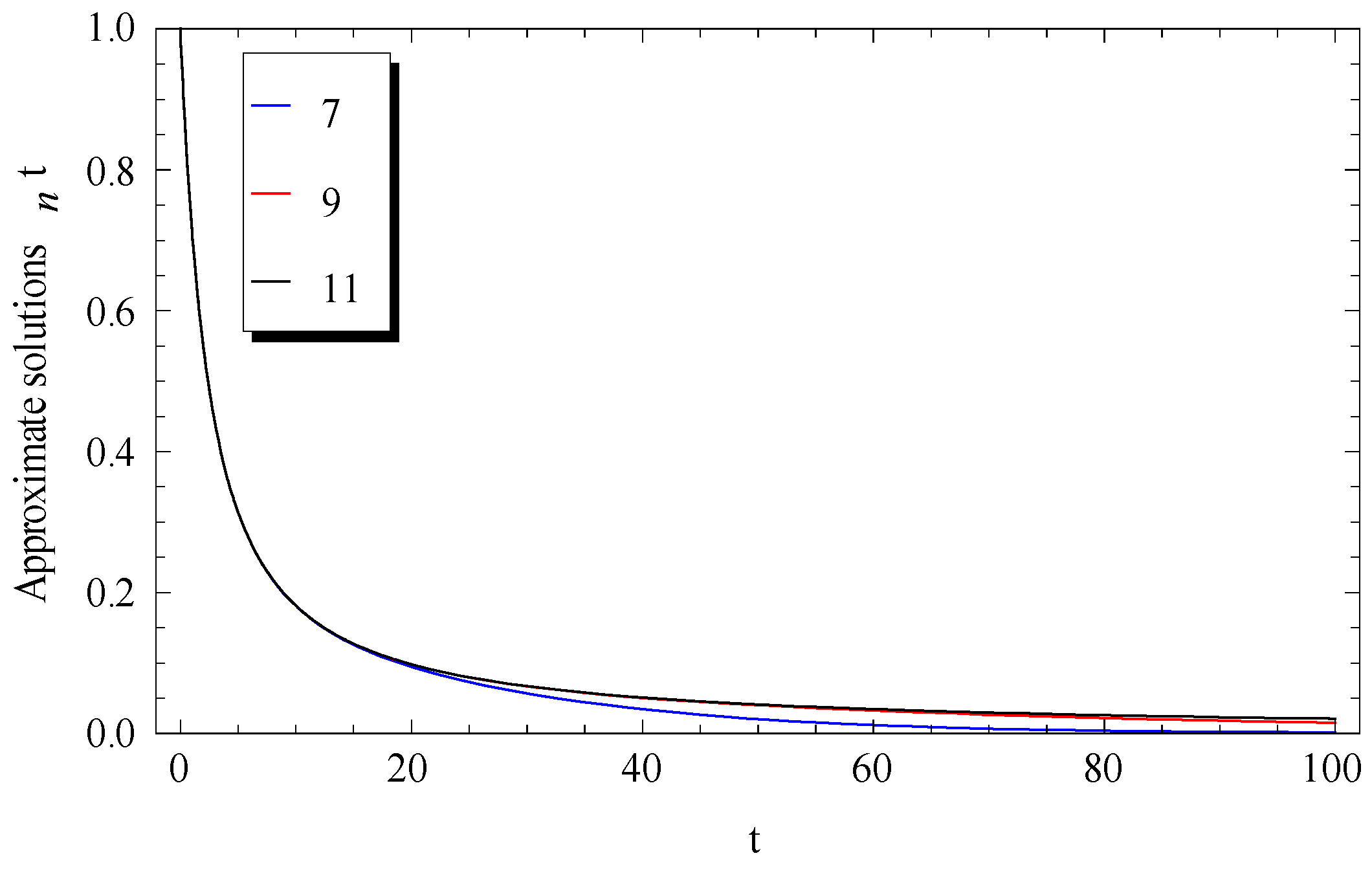
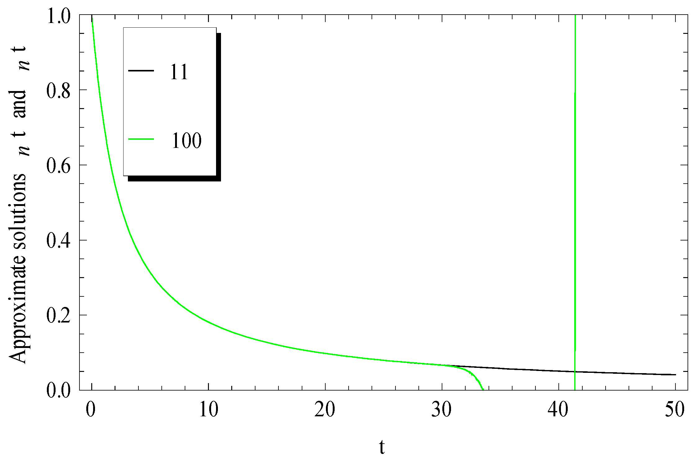
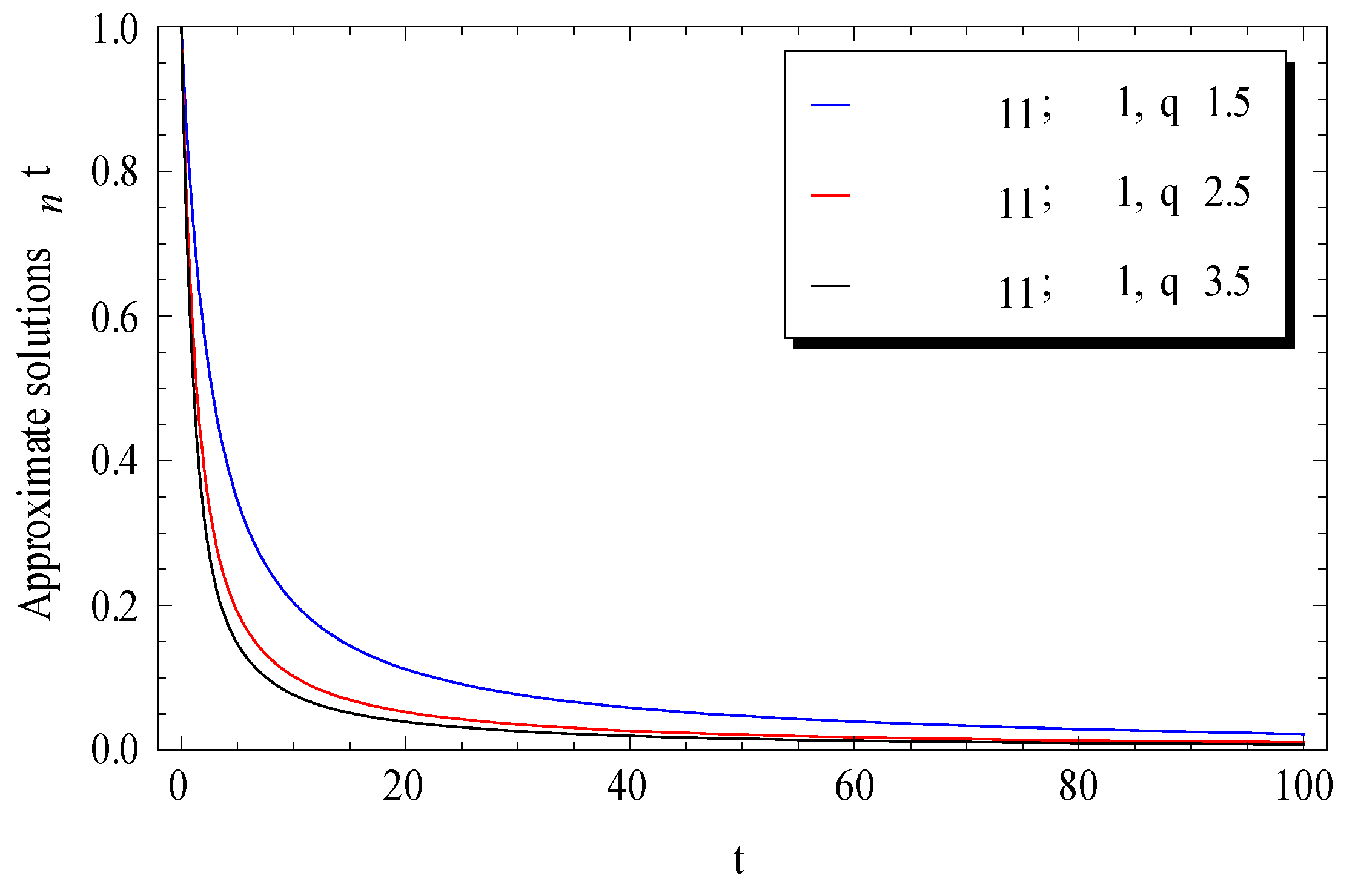
3. Comparisons and Numerical Validations

Usually, we begin by graphically demonstrating the convergence of the approximate solutions ${\mathrm{\Phi }}_n(t)$ in Equation (19). In Figure 1, Figure 2 and Figure 3, the approximate solutions ${\mathrm{\Phi }}_7(t)$, ${\mathrm{\Phi }}_9(t)$, and ${\mathrm{\Phi }}_{11}(t)$ were plotted at a fixed value of $\lambda =1$ for different values of $q$, where $q=1.5$ (Figure 1), $q=1.6$ (Figure 2), and $q=2$ (Figure 3). A rapid convergence was observed in these figures by using only a few terms of the approximate solutions. The main notice here is that the rate of convergence was increased for higher values of $q$, where at $q\ge 2$ the seven-term, nine-term, and eleven-term were nearly identical.

Hence, the eleven term approximate solution ${\mathrm{\Phi }}_{11}(t)$ of the present method was sufficient to provide a remarkably accurate solution. This will be also demonstrated later by discussing the absolute residual errors $\left|R{E}_7\right|$, $\left|R{E}_9\right|$, and $\left|R{E}_{11}\right|$. However, at the lower values of $q$ (i.e., in the domain $q\in (\mathrm{1,2})$), higher-order approximate solutions such as ${\mathrm{\Phi }}_n(t),n\ge 11$ were required to achieve high accuracy. In addition, the present approximate solutions ${\mathrm{\Phi }}_7(t)$, ${\mathrm{\Phi }}_9(t)$ and ${\mathrm{\Phi }}_{11}(t)$ were valid in the whole domain of the independent variable $t(\ge 0)$. In the literature [2], the $m$-term approximate solution was given by

$${\psi }_m(t)=\lambda \left[1+{\displaystyle \sum _{i=1}^m}\left({\displaystyle \prod _{k=1}^i}\left(q^{-k}-1\right)\right)\frac{t^i}{i!}\right],m\ge 1.$$

(29)

For purpose of comparisons with the results in the literature [2], ${\psi }_{100}$ (Equation (29) at $m=100$) was compared with the current ${\mathrm{\Phi }}_{11}(t)$ and displayed in Figure 4, Figure 5 and Figure 6 at several values of $q$.

The comparisons reveal that the present approach possesses some advantages over the previous power series one [2]. This was due to the fact that a few terms of our approximations were sufficient to achieve accurate numerical results, not only, but also in a wider range when compared with the 100-term of the previous power series solution for Equation (29).

The effects of the initial condition $\lambda$ and the delay parameter $q$ on the approximation ${\mathrm{\Phi }}_{11}(t)$ for the fluctuations of the surface brightness $y(t)$ are respectively depicted in Figure 7 and Figure 8.

It can be seen from Figure 7 that the surface brightness in the Milky Way was increased by increasing the given initial condition $\lambda$. However, a rapid decrease in surface brightness was remarked by increasing the delay parameter $q$. This latest notice revealed that the curve ${\mathrm{\Phi }}_{11}(t)$ tends faster to zero at higher values of $q$. For further validations of the current numerical results, the absolute residual error $\left|R{E}_n\right|$ defined by

$$\left|R{E}_n(t)\right|=\left|{\mathrm{\Phi }}_n^{\prime }(t)+{\mathrm{\Phi }}_n(t)-\frac{1}{q}{\mathrm{\Phi }}_n\left(\frac{t}{q}\right)\right|,n\ge 1.$$

(30)

is depicted versus $t$ in Figure 9 and Figure 10 at different values of $\lambda$ (when $q=2$) and at different values of $q$ (when $\lambda =1$), respectively.

The obtained results confirmed the accuracy of the proposed method. Moreover, the absolute residual error $\left|R{E}_{11}\right|$ approached zero even at higher values of the delay parameter $q$.

Table 1. Comparison of the present exact solution with the homotopy analysis transform method (HATM) and Daftarday-Gejji and Jafari solutions.

$\mathit{t}$	Daftarday-Gejji and Jafari Technique [2]	HATM [28]	Present: Exact
0.0	1	1	1
0.5	0.8727825992	0.8727825992	0.8729409265
1.0	0.7694328044	0.7694328044	0.7717847885
1.5	0.6788327993	0.6788327993	0.6899349261
2.0	0.5898647673	0.5898647673	0.6227083998

presents the comparison of the present exact results with those approximately obtained in Reference [2] by using Daftarday-Gejji and Jafari technique, and [28] by using the homotopy analysis transform method (HATM). We observed from Table 1 that the approximate approach in [2,28] may be close to the present exact results. This proves the several remarkable advantages of the current method over the existing methods in the literature when dealing with the Ambartsumian equation.

4. Conclusions

In this paper, an approach based on the Laplace-transform and the Adomian decomposition method (ADM) were applied on the Ambartsumian equation. This equation describes the fluctuations of surface brightness in the Milky Way. The obtained closed-form solution was reported for the first time. Numerically, it has been graphically shown that the approximate solutions in the literature were only valid in sub-domains while the present one was effective in the whole domain. Furthermore, the absolute remainder errors using a few terms of the present method tended to zero, especially, for higher values of the delay parameter q. Finally, the current approach deserves attention for higher-order linear delay differential equations. Although, the present approach was effective to exactly solve linear delay differential equations, it has limitations when it deals with non-linear delay differential equations.

References

1. Ambartsumian, V.A. On the fluctuation of the brightness of the milky way. Dokl. Akad. Nauk USSR 1994, 44, 223–226. [Google Scholar]
2. Patade, J.; Bhalekar, S. On Analytical Solution of Ambartsumian Equation. Natl. Acad. Sci. Lett. 2017. [Google Scholar] [CrossRef]
3. Kato, T.; McLeod, J.B. The functional-differential equation y’(x) = ay(λx) + by(x). Bull. Am. Math. Soc. 1971, 77, 891–935. [Google Scholar]
4. Daftardar-Gejji, V.; Bhalekar, S. Solving fractional diffusion-wave equations using the new iterative method. Fract. Calc. Appl. Anal. 2008, 11, 193–202. [Google Scholar]
5. Adomian, G.; Rach, R. On the solution of algebraic equations by the decomposition method. J. Math. Anal. Appl. 1985, 105, 141–166. [Google Scholar] [CrossRef]
6. Adomian, G.; Rach, R. Algebraic equations with exponential terms. J. Math. Anal. Appl. 1985, 112, 136–140. [Google Scholar] [CrossRef]
7. Adomian, G.; Rach, R. Algebraic computation and the decomposition method. Kybernetes 1986, 15, 33–37. [Google Scholar] [CrossRef]
8. Fatoorehchi, H.; Abolghasemi, H. Finding all real roots of a polynomial by matrix algebra and the Adomian decomposition method. J. Egypt. Math. Soc. 2014, 22, 524–528. [Google Scholar] [CrossRef]
9. Alshaery, A.; Ebaid, A. Accurate analytical periodic solution of the elliptical Kepler equation using the Adomian decomposition method. Acta Astronaut. 2017, 140, 27–33. [Google Scholar] [CrossRef]
10. Adomian, G. Solving Frontier Problems of Physics: The Decomposition Method; Kluwer Academic Publishers: Boston, MA, USA, 1994. [Google Scholar]
11. Wazwaz, A.M. Adomian decomposition method for a reliable treatment of the Bratu-type equations. Appl. Math. Comput. 2005, 166, 652–663. [Google Scholar] [CrossRef]
12. Wazwaz, A.M. The combined Laplace transform-Adomian decomposition method for handling nonlinear Volterra integro-differential equations. Appl. Math. Comput. 2010, 216, 1304–1309. [Google Scholar] [CrossRef]
13. Ebaid, A. Approximate analytical solution of a nonlinear boundary value problem and its application in fluid mechanics. Z. Naturforsch. A 2011, 66, 423–426. [Google Scholar] [CrossRef]
14. Duan, J.S.; Rach, R. A new modification of the Adomian decomposition method for solving boundary value problems for higher order nonlinear differential equations. Appl. Math. Comput. 2011, 218, 4090–4118. [Google Scholar] [CrossRef]
15. Ebaid, A. A new analytical and numerical treatment for singular two-point boundary value problems via the Adomian decomposition method. J. Comput. Appl. Math. 2011, 235, 1914–1924. [Google Scholar] [CrossRef]
16. Wazwaz, A.M.; Rach, R.; Duan, J.S. Adomian decomposition method for solving the Volterra integral form of the Lane-Emden equations with initial values and boundary conditions. Appl. Math. Comput. 2013, 219, 5004–5019. [Google Scholar] [CrossRef]
17. Ali, E.H.; Ebaid, A.; Rach, R. Advances in the Adomian decomposition method for solving two-point nonlinear boundary value problems with Neumann boundary conditions. Comput. Math. Appl. 2012, 63, 1056–1065. [Google Scholar] [CrossRef]
18. Sheikholeslami, M.; Ganji, D.D.; Ashorynejad, H.R. Investigation of squeezing unsteady nanofluid flow using ADM. Powder Technol. 2013, 239, 259–265. [Google Scholar] [CrossRef]
19. Chun, C.; Ebaid, A.; Lee, M.; Aly, E.H. An approach for solving singular two point boundary value problems: Analytical and numerical treatment. ANZIAM J. 2012, 53, 21–43. [Google Scholar] [CrossRef]
20. Kashkari, B.S.; Bakodah, H.O. New Modification of Laplace Decomposition Method for Seventh Order KdV Equation. Appl. Math. Inf. Sci. 2015, 9, 2507–2512. [Google Scholar]
21. Ebaid, A.; Aljoufi, M.D.; Wazwaz, A.-M. An advanced study on the solution of nanofluid flow problems via Adomian’s method. Appl. Math. Lett. 2015, 46, 117–122. [Google Scholar] [CrossRef]
22. Bhalekar, S.; Patade, J. An analytical solution of fishers equation using decomposition method. Am. J. Comput. Appl. Math. 2016, 6, 123–127. [Google Scholar]
23. Bakodah, H.O.; Al-Zaid, N.A.; Mirzazadeh, M.; Zhou, Q. Decomposition method for Solving Burgers’ Equation with Dirichlet and Neumann boundary conditions. Optik 2017, 130, 1339–1346. [Google Scholar] [CrossRef]
24. Bakodah, H.O.; Ebaid, A. The Adomian decomposition method for the slip flowand heat transfer of nanofluids over astretching/shrinking sheet. Rom. Rep. Phys. 2018, in press. [Google Scholar]
25. Abbaoui, K.; Cherruault, Y. Convergence of Adomian’s method applied to nonlinear equations. Math. Comput. Model. 1994, 20, 69–73. [Google Scholar] [CrossRef]
26. Cherruault, Y.; Adomian, G. Decompostion Methods: A new proof of convergence. Math. Comput. Model. 1993, 18, 103–106. [Google Scholar] [CrossRef]
27. Rach, R. A bibliography of the theory and applications of the Adomian decomposition method, 1961–2011. Kybernetes 2012, 41, 1087–1148. [Google Scholar] [CrossRef]
28. Kumar, D.; Singh, J.; Baleanu, D.; Rathore, S. Analysis of a fractional model of the Ambartsumian equation. Eur. Phys. J. Plus 2018, 133, 259. [Google Scholar] [CrossRef]
29. Spiegel, M.R. Laplac Transforms; McGraw-Hill Inc.: New York, NY, USA, 1965. [Google Scholar]
Figure 1. Convergence of the Adomian approximate solutions at λ = 1 and q = 1.5 .
Mathematics 06 00331 g001
Figure 2. Convergence of the Adomian approximate solutions at λ = 1 and q = 1.6 .
Mathematics 06 00331 g002
Figure 3. Convergence of the Adomian approximate solutions at λ = 1 and q = 2 .
Mathematics 06 00331 g003
Figure 4. Comparison between the Adomian approximate solutions and power series solution at λ = 1 and q = 1.5 .
Mathematics 06 00331 g004
Figure 5. Comparison between the Adomian approximate solutions and power series solution at λ = 1 and q = 1.6 .
Mathematics 06 00331 g005
Figure 6. Comparison between the Adomian approximate solutions and power series solution at λ = 1 and q = 2 .
Mathematics 06 00331 g006
Figure 7. Effect of initial condition λ on the Adomian approximate solutions at q = 2 .
Mathematics 06 00331 g007
Figure 8. Effect of q on the Adomian approximate solutions at λ = 1 .
Mathematics 06 00331 g008
Figure 9. Effect of initial condition λ on the absolute remainder error at q = 2 .
Mathematics 06 00331 g009
Figure 10. Effect of q on the absolute remainder error at λ = 1 .
Mathematics 06 00331 g010