On Wrapping of Quasi Lindley Distribution


1
Department of Mathematics, Al-Albayt University, Al-Mafraq 25113, Jordan
2
Department of Mathematics, Faculty of Science, Zarqa University, Zarqa 13132, Jordan
*
Author to whom correspondence should be addressed.
Mathematics 2019, 7(10), 930; https://doi.org/10.3390/math7100930
Submission received: 21 August 2019
/
Revised: 24 September 2019
/
Accepted: 26 September 2019
/
Published: 9 October 2019
Abstract
:In this paper, as an extension of Wrapping Lindley Distribution (WLD), we suggest a new circular distribution called the Wrapping Quasi Lindley Distribution (WQLD). We obtain the probability density function and derive the formula of a cumulative distribution function, characteristic function, trigonometric moments, and some related parameters for this WQLD. The maximum likelihood estimation method is used for the estimation of parameters.
1. Introduction
Directional data have many new and individual characteristics and tasks in modelling statistical analysis. It occurs in many miscellaneous fields, such as Biology, Geology, Physics, Meteorology, Psychology, Medicine, Image Processing, Political Science, Economics, and Astronomy Mardia and Jupp [1]. The wrapping of a linear distribution around the unit circle is one of the various ways in which to find a circular distribution. There are a lot of studies that have been done in this area. L’evy [2] presented wrapped distributions. Jammalamadaka and Kozubowski [3] studied circular distributions derived by wrapping the classical exponential and Laplace distributions on the real line around the circle. In 2007, Rao et al. [4] discussed wrapping of the lognormal, logistic, Weibull, and extreme-value distributions for the life testing models. Meanwhile, the wrapped weighted exponential distribution was introduced by Roy and Adnan [5]. Rao et al. [6] obtained the characteristics of a wrapped gamma distribution. Joshi and Jose [7] introduced the wrapped Lindley distribution, and they also studied the properties of the new distribution, such as characteristic function and trigonometric moments. Adnan and Roy [8] introduced the wrapped variance gamma distribution and applied it to wind direction. Lindley [9,10] suggested the Lindley distribution (LD) and he defined the probability density function (pdf) and cumulative distribution function (CDF) as follows:
while the wrapped Lindley distribution was introduced by Joshi and Jose (2018) [11]. They defined the PDF and the CDF of the wrapped LD, respectively, as follows:
Shanker and Mishra [12] derived the Quasi Lindley distribution (QLD). They introduced the QLD with two parameters, one for scale and one for shape . The (PDF) and (CDF) of (QLD), respectively, was defined as follows:
Ghitany et al. [13] established many properties of LD and proved that the LD was a better model than the exponential distribution in many ways by using a real data set. They utilized the method of maximum likelihood to provide evidence that the fit of the Lindley distribution was better. In this paper, as an extension of the Wrapping Lindley Distribution (WLD), we suggest a new circular distribution called the Wrapping Quasi Lindley Distribution (WQLD). We also obtain the probability density function and derive the formula of the cumulative distribution function, as in Section 2. In Section 3 we drive the characteristic function, which is trigonometric moments with some related parameters for this WQLD. In Section 4, the maximum likelihood estimation method is used for estimation of parameters.
2. Circular Distribution
A circular distribution is a probability distribution whose total probability is concentrated on the circumference of a unit circle (see [14]), where the points on the unit circle characterize a direction, each direction representing the values of its probabilities. The range of a circular random variable , stated in radians, may take or . There are discrete or continuous circular probability distributions which satisfy the property .
Definition 1
([14,15]). If θ is a random variable on the real with distribution function , then the random variable of the wrapped distribution satisfies the following properties:
- 1.
- and
- 2.
- .
for any integer k and is periodic.
Thus, we can define the Wrapped Quasi Lindley Distribution (WQLD) as follows:
Definition 2.
A random variable θ is said to have a Wrapped Quasi Lindley Distribution (WQLD) as follows:
It can also be simplified to:
The cumulative distribution function of WQLD can be derived as follows:
Remark 1.
We used the ratio test to check whether the series in both the PDF and CDF of WQLD converged as follows:
Figure 1 shows the circular representation of the PDF of WQLD for different values of , keeping the value for the parameter at 3.0.
The same circular representation for the PDF of WQLD with different values of , keeping the value for the parameter at 3.0 as in Figure 2.
Figure 3 shows the circular representation of the CDF of WQLD for different values of , keeping the value for the parameter at 3.0.
The same circular representation for the CDF of WQLD with different values of , keeping the value for the parameter at 3.0, as in Figure 4.
3. Characteristic Function of Wrapped Quasi Lindley Distribution
The characteristic function of for the distribution function is given by . The characteristic function for the Quasi Lindley Distribution given as follows:
Now, we can find the characteristic function of the circular model:
by
Rearranging the Equation (11), we have:
Assuming the previous integrals consist of two parts, the first part can be calculated as follows:
Now, combining both integrals I and J, we have the characteristic function of the WQLD:
We can simplify the characteristic function of the WQLD as follows:
By the trigonometric definition, we have , where and .
By some simplifications, we have
Similarly, we get and simplify the parameter , as follows:
Rearranging the entire integrals in Equation (16), we have:
4. Maximum Likehood Estimations
Here, the maximum likelihood estimators of the unknown parameters of the WQLD are derived. Let be a random sample of size n from WQLD. Then, the likelihood function is . We can define the ML as follows:
The log likelihood function is given by
Equating the partial derivative of the log-likelihood function with respect to and to zero, we get
5. Conclusions
In this paper, we introduced and studied a new kind of distribution, namely, the Wrapping Quasi Lindley Distribution (WQLD). The PDF and CDF of (WQLD) were derived and the shapes of the density function and distribution function for different values of the parameters were found by using Mathematica. An expression for the characteristic function resulted. The alternative form of the PDF of the (WQLD) was also obtained by using trigonometric moments. The parameters of (WQLD) were estimated by using the method of maximum likelihood.
Author Contributions
Investigation, A.M.H.A.-k.; Methodology, A.M.H.A.-k.; Project administration, A.M.H.A.-k.; Software, S.A.; Supervision, A.M.H.A.-k.; Writing–original draft, A.M.H.A.-k.; Writing–review and editing, S.A.
Funding
This research received no external funding.
Acknowledgments
The authors would like to acknowledge the financial support received from Al-Albayt University and Zarqa University.
Conflicts of Interest
The authors declare no conflict of interest.
References
- Mardia, K.V.; Jupp, P.E. Directional Statistics, 2nd ed.; Wiley: New York, NY, USA, 2000. [Google Scholar]
- Lévy, P.L. Addition des variables alétoires définies sur une circonférence. Bull. Soc. Math. Franc. 1939, 67, 1–41. [Google Scholar]
- Rao, S.J.; Kozubowski, T.J. New families of wrapped distributions for modeling skew circular data. Commun. Stat.-Theory Methods 2004, 33, 2059–2074. [Google Scholar]
- Rao, A.V.D.; Sarma, I.R.; Girija, S.V.S. On wrapped version of some life testing models. Commun. Stat.-Theory Methods 2007, 36, 2027–2035. [Google Scholar]
- Roy, S.; Adnan, M.A.S. Wrapped weighted exponential distributions. Stat. Probab. Lett. 2012, 82, 77–83. [Google Scholar] [CrossRef]
- Rao, A.V.D.; Girija, S.V.S.; Devaraaj, V.J. On characteristics of wrapped gamma distribution. IRACST Eng. Sci. Technol. Int. J. (ESTIJ) 2013, 3, 228–232. [Google Scholar]
- Joshi, S.; Jose, K.K.; Bhati, D. Estimation of a change point in the hazard rate of Lindley model under right censoring. Commun. Stat. Simul. Comput. 2017, 46, 3563–3574. [Google Scholar] [CrossRef]
- Adnan, M.A.S.; Roy, S. Wrapped variance gamma distribution with an application to wind direction. J. Environ. Stat. 2014, 6, 1–10. [Google Scholar]
- Lindley, D. Fiducial distributions and Bayes’ theorem. J. R. Stat. Soc. 1958, 20, 102–107. [Google Scholar] [CrossRef]
- Lindley, D. Introduction to Probability and Statistics from a Bayesian Viewpoint; Cambridge University Press: New York, NY, USA, 1981. [Google Scholar]
- Joshi, S.; Jose, K.K. Wrapped Lindley distribution. Commun. Stat. Theory Methods 2018, 47, 1013–1021. [Google Scholar] [CrossRef]
- Shanker, R.; Mishra, A. A quasi Lindley distribution. Afr. J. Math. Comput. Sci. Res. 2013, 6, 64–71. [Google Scholar]
- Ghitany, M.E.; Atieh, B.; Nadarajah, S. Lindley distribution and its application. Math. Comput. Simul. 2008, 87, 493–506. [Google Scholar] [CrossRef]
- Rao, S.J.; SenGupta, A. Topics in Circular Statistics; Series On Multivariate Analysis; World Scientific: New York, NY, USA, 2001; Volume 5. [Google Scholar] [CrossRef]
- Mardia, K.V. Statistics of Directional Data. J. R. Stat. Soc. 1975, 37, 349–393. [Google Scholar] [CrossRef]
Figure 1.
PDF of the WQLD distribution (Circular Representation), = 3.
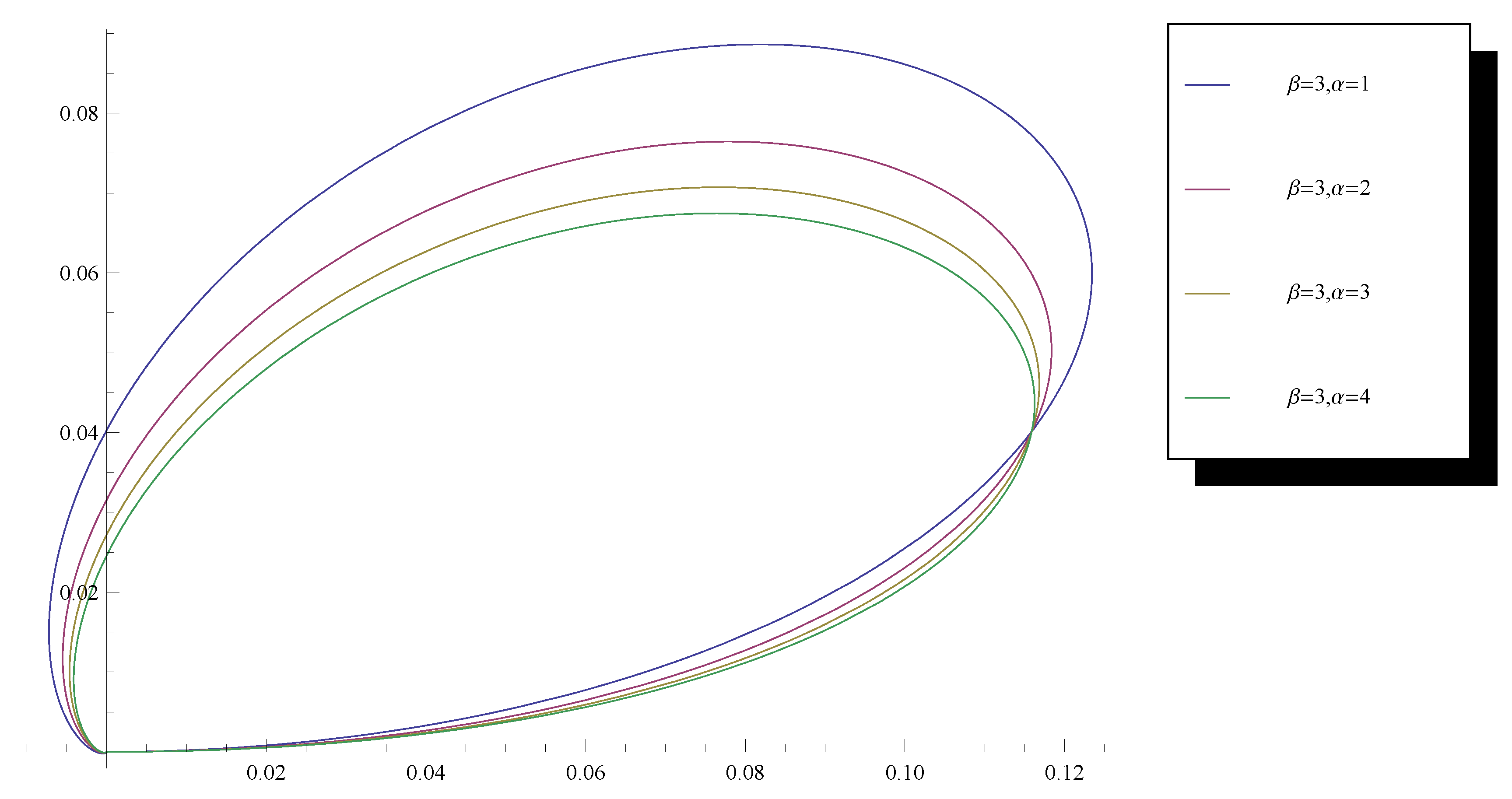
Figure 2.
PDF of the WQLD distribution (Circular Representation), = 3.
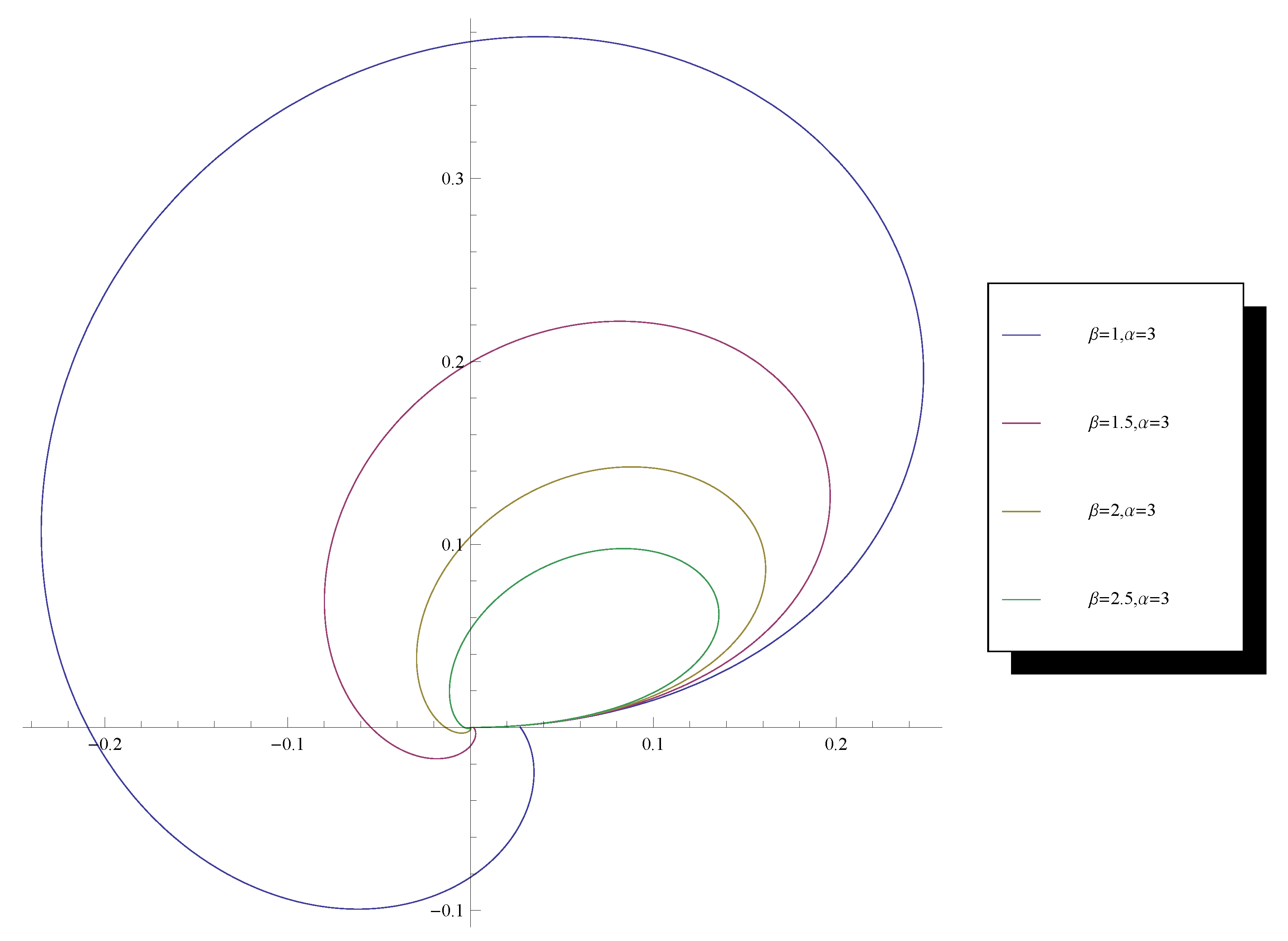
Figure 3.
CDF of the WQLD distribution (Circular Representation), = 3.

Figure 4.
CDF of the WQLD distribution (Circular Representation), = 3.

© 2019 by the authors. Licensee MDPI, Basel, Switzerland. This article is an open access article distributed under the terms and conditions of the Creative Commons Attribution (CC BY) license (http://creativecommons.org/licenses/by/4.0/).
Share and Cite
MDPI and ACS Style
Al-khazaleh, A.M.H.; Alkhazaleh, S. On Wrapping of Quasi Lindley Distribution. Mathematics 2019, 7, 930. https://doi.org/10.3390/math7100930
AMA Style
Al-khazaleh AMH, Alkhazaleh S. On Wrapping of Quasi Lindley Distribution. Mathematics. 2019; 7(10):930. https://doi.org/10.3390/math7100930
Chicago/Turabian StyleAl-khazaleh, Ahmad M. H., and Shawkat Alkhazaleh. 2019. "On Wrapping of Quasi Lindley Distribution" Mathematics 7, no. 10: 930. https://doi.org/10.3390/math7100930
Note that from the first issue of 2016, this journal uses article numbers instead of page numbers. See further details here.