Article

The Truncation Regularization Method for Identifying the Initial Value on Non-Homogeneous Time-Fractional Diffusion-Wave Equations

Department of Applied Mathematics, School of Science, Lanzhou University of Technology, Lanzhou, Gansu 730050, China
*
Author to whom correspondence should be addressed.
Mathematics 2019, 7(11), 1007; https://doi.org/10.3390/math7111007
Submission received: 26 September 2019 / Revised: 13 October 2019 / Accepted: 17 October 2019 / Published: 23 October 2019
(This article belongs to the Special Issue Numerical Analysis: Inverse Problems – Theory and Applications)

Abstract

:
In the essay, we consider an initial value question for a mixed initial-boundary value of time-fractional diffusion-wave equations. This matter is an ill-posed problem; the solution relies discontinuously on the measured information. The truncation regularization technique is used for restoring the initial value functions. The convergence estimations are given in a priori regularization parameter choice regulations and a posteriori regularization parameter choice regulations. Numerical examples are given to demonstrate this is effective and practicable.

1. Summary

Recently, abnormal diffusion has attracted intensive attention. In [1,2], we learn it has been widely used in semiconductors, nuclear magnetic resonance, quantum optics, molecular spectroscopy, porous media, polymer, turbulence, solid surface diffusion, economic, financial research, etc. The motion of normal diffusion particles is Brownian motion; its mean square and the displacement is linear with the time of movement, which is essentially a Markovian localized motion. In [3], for anomalous diffusion, it is a non-Markovian nonlocalized motion. Therefore, anomalous diffusion must take into account the long-range dependence (space) and historical dependence (time) of the motion process, so the fractional differential equation becomes an important tool for describing this process. Average migration in anomalous diffusion is non-linearly dependent on migration time. When 0 < α < 1 , the corresponding anomalous diffusion is called subdiffusion. This phenomenon exists in many systems. In [4], it exits in the transportation of charged particles in amorphous semiconductors. In [5], it exits in the porous seepage system. In [6], it exits in the vibration system in polymers. In [7], it exits in the nuclear magnetic resonance in disordered media. In [8], it exits in the transmission in fractal geometry. When 1 < α < 2 , the corresponding anomalous diffusion is called superdiffusion. This phenomenon exists in many respects. In [9], it exits in the swirl in a special region. In [10], it exits in the collective sliding diffusion on solid surface. In [11], it exits in the stratified velocity field. In [12], it exits Richardson turbulent diffusion. In [13], it exits in quantum optics. In [14], it exits in single molecule spectroscopy. In [15], it exits in the micelle system, transportation in heterogeneous rocks, etc. Based on abnormal superdiffusion of particles, in [16,17], the fractional diffusion-wave equation can accurately characterize the behavior of molecular dynamics of viscoelastic materials, mechanical, electromagnetic and biological reactions, etc. In [18], the fractional diffusion-wave equation can accurately characterize the propagation of mechanical scattering in viscoelastic media with power law creep properties. At present, there are a lot of research findings on the positive matter concerning the fractional-diffusion formula, i.e., the initial value question and initial-boundary value question. However, when solving practical problems by using the fractional diffusion equation, some boundary or initial conditions are unknown, some coefficients in the equation are unknown or the source term is unknown and some additional conditions need to be used to identify these unknown terms; this is the inverse problem of the fractional diffusion equation. For the sake of controlling pollution sources, the mathematical models concerning these problems can be reduced to the inverse problems of source term identification, initial condition reconstruction and diffusion coefficient identification of the fractional diffusion equation. Compared with the positive problems, the inverse problems are mostly ill-posed and need to be solved by the regularization method. At present, there are a lot of study achievements concerning the inverse problem for the fractional order reaction (sub-diffusion) diffusion equation, but the research for the inverse problem of the fractional order reaction (superdiffusion) diffusion equation is still in the preliminary stage. In [19], Yamamoto only gave the existence and uniqueness of solutions of the time fractional wave equation. In [20,21], Siskova considered the problem of identifying time source terms for time fractional inhomogeneous and non-linear wave equations, and this kind of problem is solved by means of the regularization method, but only the existence, uniqueness and a priori estimation formula of the solution are given, the posterior error estimation is not given. In [22], Wei proposed the inverse initial value problems for homogeneous time-fractional wave-equations, and Tikhonov was used to give the regularization; estimates of convergence rate among the regular solution and the analytical solution were given, but the error estimates were saturated. In [23], Yang et al. used the Landweber regularization method to identify the initial value for a time fractional nonhomogeneous wave equation with one measurement, but the nonhomogeneous term only depended on the spatial variable x.
Reference [22] represented a time-fractional diffusion-wave model with homogeneous Dirichlet bound conditions. In the following article, the mixed initial-boundary value problem of the time-fractional diffusion-wave nonhomogeneous equation is studied:
D t α u = u x x ( x , t ) + F ( x , t ) , 0 < x < π , 0 < t < T , u ( 0 , t ) = u ( π , t ) = 0 , 0 t T , u ( x , 0 ) = a ( x ) , 0 x π , u t ( x , 0 ) = b ( x ) , 0 x π ,
when the initial value a ( x ) and b ( x ) are known, we can solve u ( x , t ) by means of nonhomogeneous terms and boundary conditions; this is a typical direct problem. Now that the initial conditions of a ( x ) , b ( x ) are unknown, we remark that u ( x , T ) = g ( x ) , and we use a pair of measurement data ( F ( x , t ) , g ( x ) ) to invert the initial conditions of a ( x ) and b ( x ) . Here, D t α is the Caputo time-fractional derivatives with order α ( 1 < α < 2 ) , which is defined as [19]:
D t α u = α u t α : = 1 Γ ( 2 α ) 0 t u s s ( x , s ) ( t s ) α 1 d s , 1 < α < 2 ,
Γ ( x ) is the function of Gamma.
In Equation (1), the source term F ( x , t ) L ( ( 0 , T ] ; L 2 ( 0 , π ) ) and the final value g ( x ) L 2 ( 0 , π ) . The measurement data are all error-bound; assuming the measurement data functions with error are marked as F δ , g δ , they satisfy:
F δ F L ( ( 0 , T ] ; L 2 ( 0 , π ) ) δ , g δ g L 2 ( 0 , π ) δ ,
among them, δ > 0 is the error level.
The above inversion initial value problem can be decomposed into two inverse problems.
BP1: When b ( x ) is known, the unknown initial value function a ( x ) is inverted using the measured data of F δ , g δ .
BP2: When a ( x ) is known, the unknown initial value function b ( x ) is inverted using the measured data of F δ , g δ .
The truncated regularization method is used for resolving the questions BP1 and BP2. In each problem, the exact solution and conditional stability results of the problem are given. A priori error estimates and a posterior error estimates among the regular solution and the analytic solution are also presented. Finally, different numerical instances are displayed to illustrate the feasibility of the regularization mean.
The structure of this essay is as follows: The second part gives auxiliary mathematical conclusions; the third part illustrates that the problem is ill posed and gives the exact solution and conditional stability result; the fourth part gives error estimates among the regularization solutions and the analytic solution; the fifth part gives numerical consequences; and the sixth part is a summary of the article.

2. Some Auxiliary Results

In order to discuss the problem of Equation (1), this section introduces the Mittag–Leffler function and some of its properties.
Definition 1
([24,25]). For any constant α > 0 and β R , the Mittag–Leffler function is defined as:
E α , β ( z ) = k = 0 z k Γ ( α k + β ) , z C .
Lemma 1
([22]). For any λ > 0 , α > 0 and a positive constant m N , there are:
d m d t m E α , 1 ( λ t α ) = λ t α m E α , α m + 1 ( λ t α ) , t > 0 ,
d d t ( t E α , 2 ( λ t α ) ) = E α , 1 ( λ t α ) , t 0 .
Lemma 2
([23]). Let 0 < α < 2 , β R , assume μ satisfies π α 2 < μ < m i n { π , π α } , there is a constant C = C ( α , β , μ ) > 0 to make:
| E α , β ( z ) | C 1 + | z | , μ | a r g ( z ) | π .
Lemma 3
([24]). When 1 < α < 2 , β R , η > 0 , there is:
E α , β ( η ) = 1 Γ ( β α ) η + O ( 1 η 2 ) , η .

3. Exact Solution and Conditional Stability

In this section, we give the solution for Equation (1) and the properties of Mittag–Leffler functions.
Theorem 1.
Assume a , b L 2 ( 0 , π ) , F L ( ( 0 , T ] ; L 2 ( 0 , π ) ) , then the weak solutions of Equation (1) are:
u ( x , t ) = n = 1 { ( a , φ n ) E α , 1 ( n 2 t α ) + ( b , φ n ) t E α , 2 ( n 2 t α ) + 0 t E α , α ( n 2 ( t s ) α ) ( t s ) α 1 F n ( s ) d s } φ n ( x ) ,
where, u C ( [ 0 , T ] ; L 2 ( 0 , π ) ) C ( ( 0 , T ] ; H 2 ( 0 , π ) H 0 1 ( 0 , π ) ) , ( a , φ n ) represents the Fourier coefficients of a ( x ) , ( b , φ n ) represents the Fourier coefficients of b ( x ) , F n ( s ) = ( F ( x , t ) , φ n ( x ) ) , φ n ( x ) = 2 π s i n ( n x ) is a group of standard orthogonal bases under L 2 ( 0 , π ) , n = 1 , 2 , .
Define:
H p ( 0 , π ) = { ψ L 2 ( 0 , π ) ; n = 1 ( 1 + n 2 ) p | ( ψ , φ n ) | 2 < } ,
here ( · , · ) is the inner product in the sense of L 2 ( 0 , π ) , then the norm of H p ( 0 , π ) is:
ψ H p ( 0 , π ) = ( n = 1 ( 1 + n 2 ) p | ( ψ , φ n ) | 2 ) 1 2 .
Using the measurement data u ( x , T ) = g ( x ) , we acquire:
g ( x ) = u ( x , T ) = n = 1 { ( a , φ n ) E α , 1 ( n 2 T α ) + ( b , φ n ) T E α , 2 ( n 2 T α ) + 0 T E α , α ( n 2 ( T s ) α ) ( T s ) α 1 F n ( s ) d s } φ n ( x ) .
Let:
g 1 ( x ) = g ( x ) n = 1 [ ( b , φ n ) T E α , 2 ( n 2 T α ) + 0 T E α , α ( n 2 ( T s ) α ) ( T s ) α 1 F n ( s ) d s ] φ n ( x ) ,
g 2 ( x ) = g ( x ) n = 1 [ ( a , φ n ) E α , 1 ( n 2 T α ) + 0 T E α , α ( n 2 ( T s ) α ) ( T s ) α 1 F n ( s ) d s ] φ n ( x ) ,
then:
n = 1 ( a , φ n ) E α , 1 ( n 2 T α ) φ n ( x ) = g 1 ( x ) ,
n = 1 ( b , φ n ) T E α , 2 ( n 2 T α ) φ n ( x ) = g 2 ( x ) .
For the sake of solving this question, BP1 and BP2 transfer over to define the following integral equations:
K 1 ˜ a ( ξ ) : = ( 0 , π ) k 1 ˜ ( x , ξ ) a ( ξ ) d ξ = g 1 ( x ) , 0 x π ,
K 2 ˜ b ( ξ ) : = ( 0 , π ) k 2 ˜ ( x , ξ ) b ( ξ ) d ξ = g 2 ( x ) , 0 x π ,
combine Equations (13) and (14), then the kernel functions for the operators K 1 ˜ and K 2 ˜ , respectively, are:
k 1 ˜ ( x , ξ ) = n = 1 E α , 1 ( n 2 T α ) φ n ( x ) φ n ( ξ ) ,
k 2 ˜ ( x , ξ ) = n = 1 T E α , 2 ( n 2 T α ) φ n ( x ) φ n ( ξ ) .
Based on k 1 ˜ ( x , ξ ) = k 1 ˜ ( ξ , x ) and k 2 ˜ ( x , ξ ) = k 2 ˜ ( ξ , x ) , we know K 1 ˜ , K 2 ˜ are all self-adjoint operators. From [23], we know K 1 ˜ and K 2 ˜ are linear compact operators in L 2 ( 0 , π ) L 2 ( 0 , π ) , thus BP1 and BP2 are both ill-posed problems.
Let K 1 ˜ * be the adjoint operator of K 1 ˜ ; { φ n } n = 1 is a group of standard orthogonal bases on L 2 ( 0 , π ) , and we have:
K 1 ˜ * K 1 ˜ φ n ( ξ ) = E α , 1 2 ( n 2 T α ) φ n ( ξ ) ,
thus, σ n ( 1 ) = | E α , 1 ( n 2 T α ) | is the singular value of K 1 ˜ . Define:
Y n ( 1 ) ( x ) = φ n ( x ) , E α , 1 ( n 2 T α ) 0 , φ n ( x ) , E α , 1 ( n 2 T α ) < 0 .
We can see { Y n ( 1 ) } n = 1 are orthonormal on L 2 ( 0 , π ) ; then there exist:
K 1 ˜ φ n ( ξ ) = σ n ( 1 ) Y n ( 1 ) ( x ) = E α , 1 ( n 2 T α ) φ n ( x ) ,
K 1 ˜ * Y n ( 1 ) ( x ) = σ n ( 1 ) φ n ( ξ ) = E α , 1 ( n 2 T α ) Y n ( 1 ) ( ξ ) .
Thus, the singular system for the operator K 1 ˜ is ( σ n ( 1 ) ; φ n , Y n ( 1 ) ) .
The singular system for the operator K 2 ˜ is ( σ n ( 2 ) ; φ n , Y n ( 2 ) ) . In it σ n ( 2 ) = | T E α , 2 ( n 2 T α ) | :
Y n ( 2 ) ( x ) = φ n ( x ) , E α , 2 ( n 2 T α ) 0 , φ n ( x ) , E α , 2 ( n 2 T α ) < 0 ,
Lemma 4
([22]). When 1 < α < 2 , T > 0 is a given constant, there are finite points to make E α , 1 ( n 2 T α ) = 0 and E α , 2 ( n 2 T α ) = 0 , respectively. Note the point set to let E α , 1 ( n 2 T α ) = 0 is I 1 = { n 1 , n 2 , n 3 , , n N } , the point set to let E α , 2 ( n 2 T α ) = 0 is I 2 = { m 1 , m 2 , m 3 , , m M } .
Proof. 
According to Lemma 3, there exists L 0 > 0 to make:
E α , 1 ( n 2 T α ) 1 2 Γ ( 1 α ) n 2 T α < 0 , n 2 T α > L 0 ,
if 1 < α < 2 , then we have E α , 1 ( n 2 T α ) = 0 only under n 2 T α L 0 . Then for lim n + n 2 = + there exits finite points n to satisfy n 2 T α L 0 . The proof of E α , 2 ( n 2 T α ) is similar to the above process. □
Remark 1.
When I 1 = ϕ , I 2 = ϕ , the kernel functions for K 1 ˜ are as in Equation (17), the kernel function for K 2 ˜ is as in Equation (18). In this paper, this situation is regarded as a special case.
Next we talk about the general situation, which is: I 1 ϕ , I 2 ϕ . When I 1 ϕ , I 2 ϕ , the kernel function for K 1 ˜ and K 2 ˜ are, respectively, expressed as,
k 1 ˜ ( x , ξ ) = n = 1 , n I 1 E α , 1 ( n 2 T α ) φ n ( x ) φ n ( ξ ) ,
k 2 ˜ ( x , ξ ) = n = 1 , n I 2 T E α , 2 ( n 2 T α ) φ n ( x ) φ n ( ξ ) .
Then, the kernel space for the operator K 1 ˜ is, when I 1 ϕ :
N ( K 1 ˜ ) = s p a n { φ n ; n I 1 } .
when I 1 = ϕ :
N ( K 1 ˜ ) = { 0 } .
The kernel space for the operator K 2 ˜ is, when I 2 ϕ :
N ( K 2 ˜ ) = s p a n { φ n ; n I 2 } ,
when I 2 = ϕ :
N ( K 2 ˜ ) = { 0 } ,
The ranges for K 1 ˜ and K 2 ˜ are, respectively, written as:
R ( K 1 ˜ ) = { g 1 L 2 ( 0 , π ) | ( g 1 , φ n ) = 0 , n I 1 ; n = 1 , n I 1 ( ( g 1 , φ n ) E α , 1 ( n 2 T α ) ) 2 < + } ,
R ( K 2 ˜ ) = { g 2 L 2 ( 0 , π ) | ( g 2 , φ n ) = 0 , n I 2 ; n = 1 , n I 2 ( ( g 2 , φ n ) T E α , 2 ( n 2 T α ) ) 2 < + } .
Lemma 5
([22]). When 1 < α < 2 , there exist positive constants C ̲ and C ¯ which only rely on α, T and n 2 to make:
C ̲ n 2 | E α , 1 ( n 2 T α ) | C ¯ n 2 , n I 1 ,
C ̲ n 2 | E α , 2 ( n 2 T α ) | C ¯ n 2 , n I 2 .
Theorem 2.
When I 1 , g 1 R ( K 1 ˜ ) , the integral Equation (15) has infinite solutions, but in L 2 ( 0 , π ) it has only one optimal approximate solution:
a ( x ) = n = 1 , n I 1 ( g 1 , φ n ) E α , 1 ( n 2 T α ) φ n ( x ) ,
when I 1 = , g 1 R ( K 1 ˜ ) , the exact solution for BP1 is:
a ( x ) = n = 1 ( g 1 , φ n ) E α , 1 ( n 2 T α ) φ n ( x ) .
Proof. 
Making use of Equation (15), it is easy to get the above conclusion. □
Theorem 3.
When I 2 and g 2 R ( K 2 ˜ ) , the integral Equation (16) has infinite solutions, but in L 2 ( 0 , π ) it has only one optimal approximate solution:
b ( x ) = n = 1 , n I 2 ( g 2 , φ n ) T E α , 2 ( n 2 T α ) φ n ( x ) ,
when I 2 = , g 2 R ( K 2 ˜ ) , the exact solution for BP2 is:
b ( x ) = n = 1 ( g 2 , φ n ) T E α , 2 ( n 2 T α ) φ n ( x ) .
Proof. 
Making use of Equation (16), it is easy to get the above conclusion. □
Define an a priori boundary for any a ( x ) H p ( 0 , π ) N ( K 1 ˜ ) and we have:
a H p ( 0 , π ) E 1 , p > 0 , E 1 > 0 ,
and for any b ( x ) H p ( 0 , π ) N ( K 2 ˜ ) , we have:
b H p ( 0 , π ) E 2 , p > 0 , E 2 > 0 .
Theorem 4.
For any a ( x ) H p ( 0 , π ) N ( K 1 ˜ ) which satisfies Equation (25), we get:
a C 1 K 1 ˜ a p p + 2 E 1 2 p + 2 ,
in it, C 1 = C ̲ p p + 2 .
Proof. 
For any a ( x ) H p ( 0 , π ) N ( K 1 ˜ ) , there is:
a = n = 1 , n I 1 ( a , φ n ) φ n .
By K 1 ˜ a 2 = n = 1 , n I 1 E α , 1 2 ( n 2 T α ) ( a , φ n ) 2 , Lemma 5 and the inequality of H o ¨ lder, we obtain:
a 2 = n = 1 , n I 1 ( a , φ n ) 2 n = 1 , n I 1 ( | E α , 1 ( n 2 T α ) | ( a , φ n ) ) 4 p + 2 E α , 1 2 ( n 2 T α ) ( | E α , 1 ( n 2 T α ) | ( a , φ n ) ) 2 p p + 2 ( n = 1 , n I 1 ( a , φ n ) 2 | E α , 1 p ( n 2 T α ) | ) 2 p + 2 × ( n = 1 , n I 1 | E α , 1 ( n 2 T α ) | 2 ( a , φ n ) 2 ) p p + 2 ( n = 1 , n I 1 ( ( n 2 C ̲ ) p ( a , φ n ) 2 ) ) 2 p + 2 K 1 ˜ a 2 p p + 2 C ̲ 2 p p + 2 E 1 4 p + 2 K 1 ˜ a 2 p p + 2 .
So:
a C ̲ p p + 2 K 1 ˜ a p p + 2 E 1 2 p + 2 .
 □
Theorem 5.
For any b ( x ) H p ( 0 , π ) N ( K 2 ˜ ) that satisfies Equation (26), we get:
b ( T C ̲ ) p p + 2 K 2 ˜ b p p + 2 E 2 2 p + 2 .
Proof. 
The method of proof is consistent with Theorem 4. There is no further elaboration here. □

4. Regular Solutions and Error Estimations

Consulting [26,27,28], regular solutions of BP1 and BP2 are given by the truncated regularization method. Based on the singular systems of linear compact operators K ˜ 1 and K ˜ 2 :
a N 1 δ ( x ) = n = 1 , n I 1 N 1 ( g 1 δ , φ n ) E α , 1 ( n 2 T α ) φ n ( x ) ,
In this, N 1 is the regularization parameter,
g 1 δ = g δ n = 1 [ ( b , φ n ) T E α , 2 ( n 2 T α ) + 0 T E α , α ( n 2 ( T s ) α ) ( T s ) α 1 F n δ ( s ) d s ] φ n .
b N 2 δ ( x ) = n = 1 , n I 2 N 2 ( g 2 δ , φ n ) T E α , 2 ( n 2 T α ) φ n ( x ) ,
In this, N 2 is the regularization parameter:
g 2 δ = g δ n = 1 [ ( a , φ n ) E α , 1 ( n 2 T α ) + 0 T E α , α ( n 2 ( T s ) α ) ( T s ) α 1 F n δ ( s ) d s ] φ n .
Next, the convergence estimate among the optimal approximate solution a ( x ) and the regular solution a N 1 δ ( x ) is given under the a priori regularization parameter selection rule.
Lemma 6
([29]). Suppose F L ( ( 0 , T ] ; L 2 ( 0 , π ) ) , 0 < d < 4 , there is a constant M to make:
g ( x ) n = 1 0 T E α , α ( n 2 ( T s ) α ) ( T s ) α 1 F n ( s ) d s φ n ( x ) , 2 ( g 2 + M F L ( ( 0 , T ] ; L 2 ( 0 , π ) ) 2 ) ,
In this, F n ( s ) = ( F ( x , t ) , φ n ( x ) ) , the constant M = 1 c 2 n = 1 1 n 4 d and c is a positive constant which only relies on n.
Define an orthogonal projection operator Q 1 : L 2 ( 0 , π ) R ( K 1 ˜ ) ¯ , making use of Equations (3) and (31), we have:
Q 1 g 1 δ Q 1 g 1 g 1 δ g 1 = g 1 δ g 1 2 ( M + 1 ) δ .
Define an orthogonal projection operator Q 2 : L 2 ( 0 , π ) R ( K 2 ˜ ) ¯ ; making use of Equations (3) and (31), we have:
Q 2 g 2 δ Q 2 g 2 g 2 δ g 2 = g 2 δ g 2 2 ( M + 1 ) δ .
Theorem 6.
a ( x ) is as in Equation (21); the regularization solution a N 1 δ ( x ) is as in Equation 29); assuming a ( x ) satisfies Equation (25) and the measurement error hypothesis Equation (3) is held, then the regular parameter is:
N 1 = [ ( E 1 δ ) 1 p + 2 ] ,
In this, [ ( E 1 δ ) 1 p + 2 ] is the biggest integer and is no more than ( E 1 δ ) 1 p + 2 , the estimate between a ( x ) and a N 1 δ ( x ) is:
a N 1 δ a C 2 δ p p + 2 E 1 2 p + 2 ,
In this, C 2 = 1 + 2 ( M + 1 ) C ̲ .
Proof. 
By the trigonometric inequality, we have:
a N 1 δ a a N 1 δ a N 1 + a N 1 a .
First, we prove that the first term is derived from Lemmas 5 and 6:
a N 1 δ a N 1 2 = n = 1 , n I 1 N 1 ( g 1 n g 1 δ n E α , 1 ( n 2 T α ) ) φ n ( x ) 2 [ sup 1 n N 1 , n I 1 ( 1 E α , 1 ( n 2 T α ) ) ] 2 × n = 1 , n I 1 N 1 ( g 1 n g 1 δ n ) 2 [ sup 1 n N 1 , n I 1 ( 1 C ̲ n 2 ) ] 2 ( 2 ( M + 1 ) ) δ 2 2 ( M + 1 ) C ̲ 2 [ sup 1 n N 1 , n I 1 n 2 ] 2 δ 2 2 ( M + 1 ) C ̲ 2 N 1 4 δ 2 .
In this, g 1 n = ( g 1 , φ n ) , g 1 δ n = ( g 1 δ , φ n ) . Then:
a N 1 δ a N 1 2 ( M + 1 ) C ̲ N 1 2 δ .
According to Equation (25), we estimate the second term of trigonometric inequality:
a N 1 a 2 = n = N 1 + 1 , n I 1 ( g 1 n E α , 1 ( n 2 T α ) ) φ n ( x ) 2 = n = N 1 + 1 , n I 1 ( a n ) 2 = n = N 1 + 1 , n I 1 ( a n ( 1 + n 2 ) p 2 ( 1 + n 2 ) p 2 ) 2 [ sup n N 1 + 1 , n I 1 ( ( 1 + n 2 ) p 2 ) ] 2 E 1 2 N 1 2 p E 1 2 .
Thus:
a N 1 a N 1 p E 1 .
Then:
a N 1 δ a C 2 δ p p + 2 E 1 2 p + 2 ,
In this, C 2 = 1 + 2 ( M + 1 ) C ̲ .
Next, the rule of parameter selection for posterior error regularization is given by the Morozov principle. We define the following operator:
P 1 m g 1 δ = n = 1 , n I 1 m g 1 n δ φ n ( x ) ,
and select the regularization parameter to satisfy:
( Q 1 P 1 N 1 ) g 1 δ τ 1 δ ( Q 1 P 1 N 1 1 ) g 1 δ ,
In this, τ 1 > 2 ( M + 1 ) is a constant, Q 1 g 1 δ > τ 1 δ > 0 . □
Lemma 7.
Suppose ρ ( N 1 ) : = ( Q 1 P 1 N 1 ) g 1 δ ; it has the following properties:
(a) 
ρ ( N 1 ) is a successive function;
(b) 
lim N 1 0 ρ ( N 1 ) = Q 1 g 1 δ ;
(c) 
lim N 1 ρ ( N 1 ) = 0 ;
(d) 
ρ ( N 1 ) is a strictly decreasing function.
Lemma 8.
Suppose Equations (3) and (25) are held, then the regularization parameter N 1 is obtained by the posterior regularization parameter selection rule, and we have:
N 1 C ¯ 1 p + 2 ( E 1 ( τ 1 2 ( M + 1 ) ) δ ) 1 p + 2 .
Proof. 
On the one hand, according to Lemma 5 and Equations (15) and (35), we have:
( Q 1 P 1 N 1 1 ) g 1 2 = n = N 1 , n I 1 ( g 1 n ) φ n ( x ) 2 = n = N 1 , n I 1 ( a n E α , 1 ( n 2 T α ) ) 2 = n = N 1 , n I 1 ( a n E α , 1 ( n 2 T α ) ( 1 + n 2 ) p 2 ( 1 + n 2 ) p 2 ) 2 [ sup n N 1 , n I 1 ( ( 1 + n 2 ) p 2 ( E α , 1 ( n 2 T α ) ) ) ] 2 × n = N 1 , n I 1 ( a n ( 1 + n 2 ) p 2 ) 2 [ sup n N 1 , n I 1 ( ( 1 + n 2 ) p 2 ( C ¯ n 2 ) ) ] 2 E 1 2 C ¯ 2 1 N 1 2 p + 4 E 1 2 ,
then:
( Q 1 P 1 N 1 1 ) g 1 C ¯ N 1 ( p + 2 ) E 1 .
On the other hand, according to Lemma 6 and Equation (36), we have:
( Q 1 P 1 N 1 1 ) g 1 = ( P 1 N 1 1 Q 1 ) g 1 δ ( Q 1 P 1 N 1 1 ) ( g 1 g 1 δ ) ( P 1 N 1 1 Q 1 ) g 1 δ ( Q 1 P 1 N 1 1 ) ( g 1 g 1 δ ) τ 1 δ 2 ( M + 1 ) δ = ( τ 1 2 ( M + 1 ) ) δ ,
then:
( Q 1 P 1 N 1 1 ) g 1 ( τ 1 2 ( M + 1 ) ) δ .
Combine Equations (38) and (39); then:
N 1 C ¯ 1 p + 2 ( E 1 ( τ 1 2 ( M + 1 ) ) δ ) 1 p + 2 .
 □
Lemma 9.
Suppose a N 1 δ ( x ) is a regular solution of BP1 corresponding to measurement data with errors and a N 1 ( x ) is the regular solution corresponding to the measurement data without errors; then we have:
a N 1 δ a N 1 C 3 ( τ 1 2 ( M + 1 ) ) 2 p + 2 δ p p + 2 E 1 2 p + 2 ,
In this, C 3 = ( C 2 1 ) C ¯ 2 p + 2 .
Proof. 
Applying Equation (33) and Lemma 8, we get:
a N 1 δ a N 1 N 1 2 δ 2 ( M + 1 ) C ̲ ( C ¯ 1 p + 2 ( E 1 ( τ 1 2 ( M + 1 ) ) δ ) 1 p + 2 ) 2 δ 2 ( M + 1 ) C ̲ = 2 ( M + 1 ) C ̲ C ¯ 2 p + 2 ( τ 1 2 ( M + 1 ) ) 2 p + 2 δ p p + 2 E 1 2 p + 2 = ( C 2 1 ) C ¯ 2 p + 2 ( τ 1 2 ( M + 1 ) ) 2 p + 2 δ p p + 2 E 1 2 p + 2 = C 3 ( τ 1 2 ( M + 1 ) ) 2 p + 2 δ p p + 2 E 1 2 p + 2 .
 □
Lemma 10.
a ( x ) is as in Equation (21) and a N 1 ( x ) is the regular solution corresponding to the measurement data without errors; suppose Equation (3) and the a priori boundary Equation (25) are held; then we have:
a N 1 a C 1 ( τ 1 + 2 ( M + 1 ) ) p p + 2 δ p p + 2 E 1 2 p + 2 .
Proof. 
Making use of Lemmas 5 and 6, Equation (36) and the H o ¨ lder inequality, we obtain:
a N 1 a 2 = n = 1 , n I 1 N 1 ( g 1 n E α , 1 ( n 2 T α ) ) φ n ( x ) n = 1 , n I 1 ( g 1 n E α , 1 ( n 2 T α ) ) φ n ( x ) 2 = n = N 1 + 1 , n I 1 ( g 1 n E α , 1 ( n 2 T α ) ) 2 = n = N 1 + 1 , n I 1 ( g 1 n p p + 2 g 1 n 2 p + 2 E α , 1 ( n 2 T α ) ) 2 ( n = N 1 + 1 , n I 1 ( g 1 n 2 p p + 2 ) p + 2 p ) p p + 2 ( n = N 1 + 1 , n I 1 ( g 1 n 4 p + 2 E α , 1 2 ( n 2 T α ) ) p + 2 2 ) 2 p + 2 = ( n = N 1 + 1 , n I 1 ( g 1 n ) 2 ) p p + 2 ( n = N 1 + 1 , n I 1 ( g 1 n 2 1 E α , 1 p + 2 ( n 2 T α ) ) ) 2 p + 2 ( n = N 1 + 1 , n I 1 ( g 1 n g 1 n δ + g 1 n δ ) ) 2 p p + 2 ( n = N 1 + 1 , n I 1 ( a n 2 1 E α , 1 p ( n 2 T α ) ) ) 2 p + 2 ( 2 ( M + 1 ) δ + τ 1 δ ) 2 p p + 2 ( n = N 1 + 1 , n I 1 ( a n 2 ( 1 + n 2 ) p 1 E α , 1 p ( n 2 T α ) ( 1 + n 2 ) p ) ) 2 p + 2 ( 2 ( M + 1 ) δ + τ 1 δ ) 2 p p + 2 E 1 4 p + 2 ( sup n N 1 + 1 , n I 1 1 ( 1 + n 2 ) p E α , 1 p ( n 2 T α ) ) 2 p + 2 ( 2 ( M + 1 ) δ + τ 1 δ ) 2 p p + 2 E 1 4 p + 2 ( sup n N 1 + 1 , n I 1 1 ( 1 + n 2 ) p ( C ̲ n 2 ) p ) 2 p + 2 ( 2 ( M + 1 ) + τ 1 ) 2 p p + 2 ( 1 C ̲ ) 2 p p + 2 δ 2 p p + 2 E 1 4 p + 2 .
Then:
a N 1 a ( 1 C ̲ ) p p + 2 ( τ 1 + 2 ( M + 1 ) ) p p + 2 δ p p + 2 E 1 2 p + 2 .
 □
Theorem 7.
Suppose Equation (3) and the a priori boundary Equation (25) are held and the regularization parameter is given by Equation (36); then the a posteriori estimation between a ( x ) and a N 1 δ ( x ) is:
a N 1 δ a [ C 3 ( τ 1 2 ( M + 1 ) ) 2 p + 2 + C 1 ( τ 1 + 2 ( M + 1 ) ) p p + 2 ] δ p p + 2 E 1 2 p + 2 .
Proof. 
By aid of trigonometric inequality and Equations (40) and (41), we get:
a N 1 δ a = a N 1 δ a N 1 + a N 1 a a N 1 δ a N 1 + a N 1 a C 3 ( τ 1 2 ( M + 1 ) ) 2 p + 2 δ p p + 2 E 1 2 p + 2 + C 1 ( τ 1 + 2 ( M + 1 ) ) p p + 2 δ p p + 2 E 1 2 p + 2 = [ C 3 ( τ 1 2 ( M + 1 ) ) 2 p + 2 + C 1 ( τ 1 + 2 ( M + 1 ) ) p p + 2 ] δ p p + 2 E 1 2 p + 2 .
 □
The following theorems give a priori error estimates and a posteriori error estimates of problem BP2. The proof method is similar to problem BP1, so only the result is given and the proof process is not given.
Theorem 8.
b ( x ) is as in Equation (23) and b N 2 δ ( x ) is the regular solution corresponding to the measured data with errors; assuming Equations (3) and (26) are held, then the regularization parameter is:
N 2 = [ ( E 2 δ ) 1 p + 2 ]
In this, [ ( E 2 δ ) 1 p + 2 ] is the biggest integer and is no more than ( E 2 δ ) 1 p + 2 ; the estimate is:
b N 2 δ b C 4 δ p p + 2 E 2 2 p + 2 ,
In this, C 4 = 1 + 2 ( M + 1 ) C ̲ T .
A posteriori error estimates of b ( x ) are given by the Morozov principle. We define the following operator:
P 2 m g 2 δ = n = 1 , n I 2 m g 2 δ n φ n ( x ) ,
In this, g 2 δ n = ( g 2 δ , φ n ) ; select regularization parameters to satisfy:
( Q 2 P 2 N 2 ) g 2 δ τ 2 δ ( Q 2 P 2 N 2 1 ) g 2 δ ,
In this, τ 2 > 2 ( M + 1 ) is a constant. Similar to Lemma 4.3, suppose Q 2 g 2 δ > τ 2 δ .
Theorem 9.
b ( x ) is as in Equation (23) and b N 2 δ ( x ) is the regular solution corresponding to the measured data with errors; suppose Equations (3) and (26) are held, if the regularization parameter is given by Equation (45), the error estimate is:
b N 2 δ b [ C 5 ( τ 2 2 ( M + 1 ) ) 2 p + 2 + C 6 ( τ 2 + 2 ( M + 1 ) ) p p + 2 ] δ p p + 2 E 2 2 p + 2 ,
In this, C 5 = ( T C ¯ ) 2 p + 2 ( C 4 1 ) , C 6 = ( 1 T C ̲ ) p p + 2 .

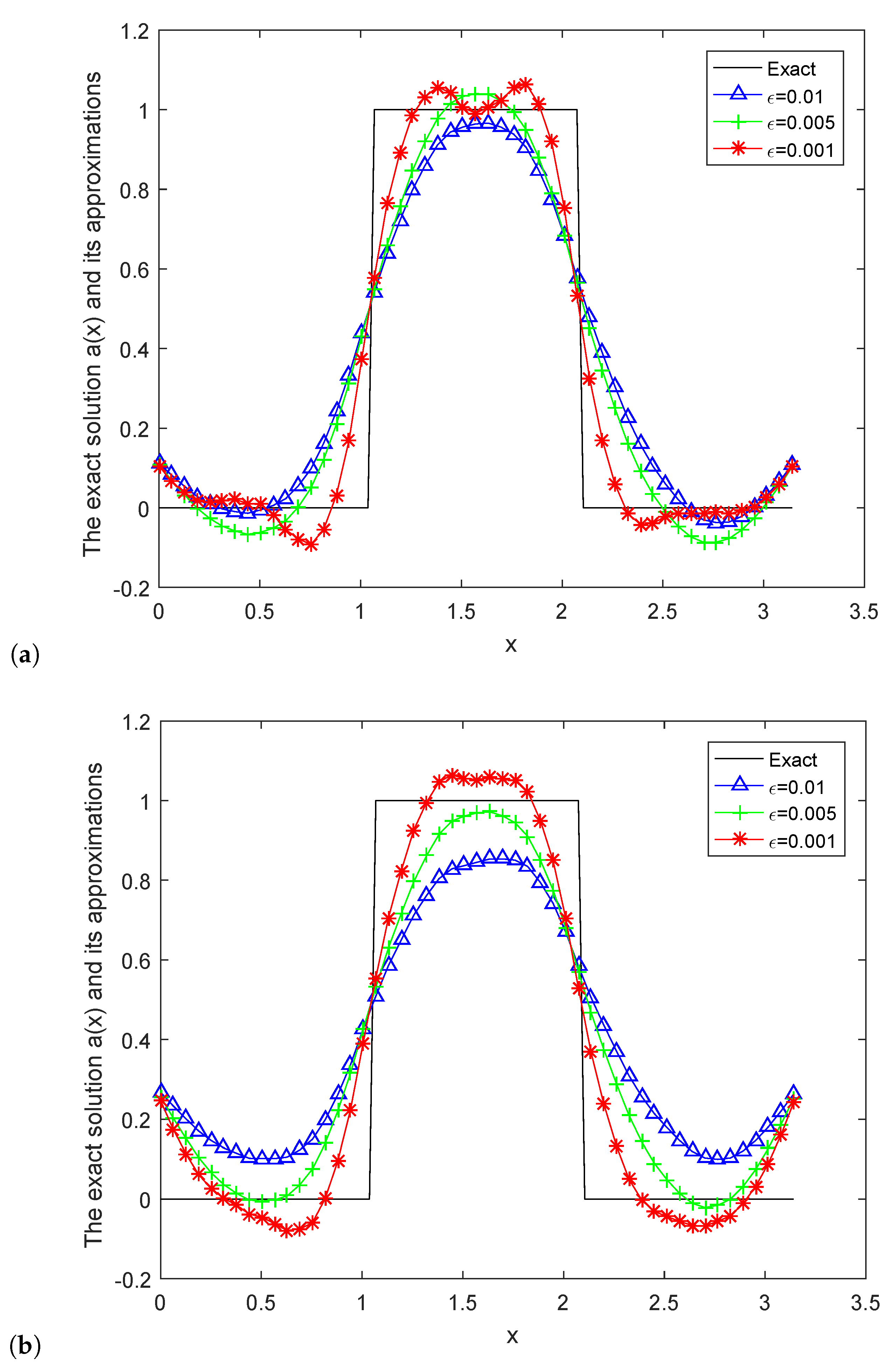
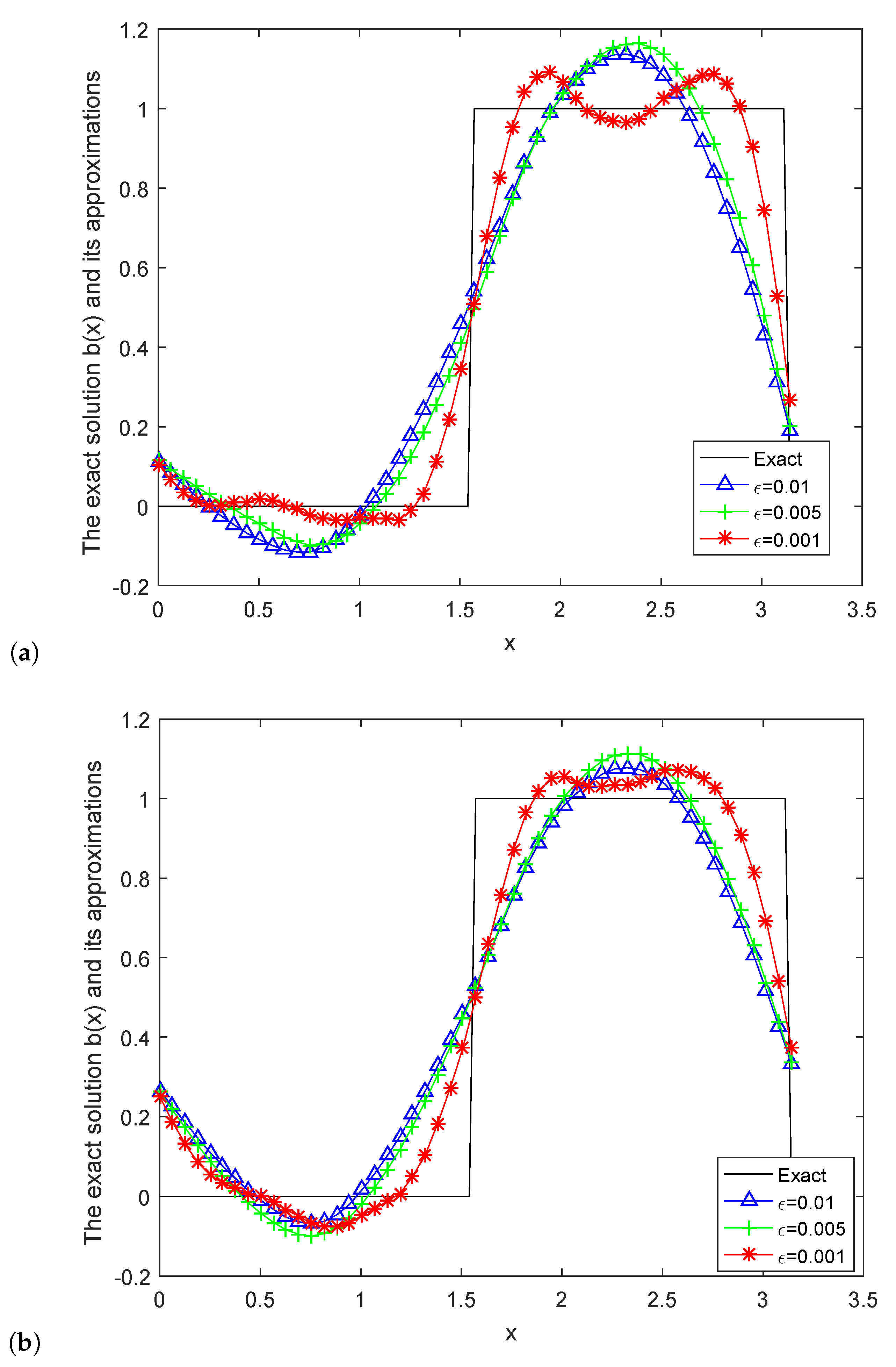
5. Numerical Implementation

In this section, different numeric instances are selected to illustrate the effectiveness of the truncated regularization technique for inversion of initial value functions concerning the time-fractional nonhomogeneous wave equation.
By resolving the direct question of Equation (1), we get the measurement information g ( x ) ,
D t α u = u x x ( x , t ) + F ( x , t ) , 0 < x < π , 0 < t < T , u ( 0 , t ) = u ( π , t ) = 0 , 0 t T , u ( x , 0 ) = a ( x ) , 0 x π , u t ( x , 0 ) = b ( x ) , 0 x π ,
The finite difference method is used to discretize the above equation; the step for time and space are Δ t = T N and Δ x = π M . Thus, we apply t n = n Δ t ( n = 0 , 1 , 2 , , N ) to represent the grid point in time domain [ 0 , T ] and we apply x i = i Δ x ( n = 0 , 1 , 2 , , M ) to represent the grid point in space domain [ 0 , π ] . The approximate value of each grid point u is denoted u i n u ( x i , t n ) . Referring to [30], we can write the discrete form of the time-fractional derivative:
D t α u i n = ( Δ t ) α Γ ( 3 α ) ( u i n u i n 1 ) ( Δ t ) α Γ ( 3 α ) j = 1 n 1 ( B n j 1 B n j ) ( u i j u i j 1 ) ( Δ t ) 1 α Γ ( 3 α ) B n 1 b ( x i ) ,
here B k = ( k + 1 ) 2 α k 2 α , k = 0 , 1 , 2 , . The final value g ( x ) is calculated by combining the measured non-homogeneous term F ( x , t ) . The R a n d n ( · ) function is used to add random perturbations to g ( x ) and F ( x , t ) :
g δ = g + ε ( 2 r a n d n ( s i z e ( g ) ) 1 ) , F δ = F + ε ( 2 r a n d n ( s i z e ( F ) ) 1 ) .
where, the absolute error among the analytic solution and the regularized solution are:
e a 1 = 1 ( M + 1 ) i = 1 M + 1 ( a i a i N 1 , δ ) 2 , e a 2 = 1 ( M + 1 ) i = 1 M + 1 ( b i b i N 2 , δ ) 2 .
Because the a priori bound is not well defined, only the numerical results under the rules of selecting a posteriori regularization parameters are given here. In the next instances, M = 100 , N = 50 , F ( x , t ) = ( 1 + x 2 ) e x p ( t ) and T = 1 ; for the sake of inverting the unknown function a ( x ) , we order b ( x ) = s i n ( 6 π x ) ; for the sake of inverting the unknown b ( x ) , we order a ( x ) = x s i n ( x ) .
Figure 1 shows the absolute error between the exact solution a ( x ) and the regularized solution under α = 1.2 and various ε for Instance 1. Figure 2 shows the exact solution a ( x ) and the regularized solution for Instance 1 with difference α . Figure 3 shows the exact solution a ( x ) and the regularized solution for Instance 2 with difference α Figure 4 shows the exact solution a ( x ) and the regularized solution for Instance 3 with difference α Figure 5 shows the exact solution b ( x ) and the regularized solution for Instance 4 with difference α Figure 6 shows the exact solution b ( x ) and the regularized solution for Instance 5 with difference α Figure 7 shows the exact solution b ( x ) and the regularized solution for Instance 6 with difference α .
Instance 1.
Let:
a ( x ) = x s i n ( x ) .
Table 1 shows the relative error between the exact solution and the regularization solution as α increases. From Table 1, we can see the relative error between the exact solution and the regularization solution increases as α increases.
Instance 2.
Let:
a ( x ) = 2 x ( 0 < x < π 2 ) + 2 ( π x ) ( π 2 x < π ) .
Instance 3.
Let:
a ( x ) = 0 ( 0 < x < π 3 ) + 1 ( π 3 x < 2 π 3 ) + 0 ( 2 π 3 x < π ) .
Instance 4.
Let:
b ( x ) = 2 s i n ( x ) .
Instance 5.
Let:
b ( x ) = 0 ( 0 < x π 4 ) + 4 ( x π 4 ) ( π 4 < x π 2 ) 4 ( x 3 π 4 ) ( π 2 < x 3 π 4 ) + 0 ( 3 π 4 < x π ) .
Instance 6.
Let:
b ( x ) = 0 ( 0 < x π 2 ) + 1 ( π 2 < x π ) .
As can be seen from the numerical examples above, the smaller the time order α and noise level ε , the better the numerical results will be. Examples 1 and 4 outperform Examples 2, 3, 5 and 6, because their functions are better chosen.

6. Conclusions

In this paper, we study the question of the inversion of initial information for the time-fractional nonhomogeneous diffusion-wave formula, and choose truncated regularization means to resolve this question. The exact solution, conditional stability and a priori and a posteriori error estimates are given; some suitable numerical instances are selected to show the validity of this method. Compared with other scholars’ work, the convergence estimates in this paper are not saturated, and the non-homogeneous terms are both related to time and space. At the same time, combined with graphs and tables, the numerical results illustrate that the smaller the order α and noise level ε , the better the numerical results will be.

Author Contributions

The main idea of this paper was proposed by F.Y. and Q.P. prepared the manuscript initially and performed all the steps of the proofs in this research. Conceptualization, X.-X.L. and D.-G.L. All authors read and approved the final manuscript.

Funding

The project is supported by the National Natural Science Foundation of China (No.11561045), the Doctor Fund of Lan Zhou University of Technology.

Conflicts of Interest

The authors declare that they have no conflict of interest.

References

  1. Metzler, R.; Klafter, J. The random walk’s guide to anomalous diffusion: A fractional dynamics approach. Phys. Rep. 2000, 339, 1–77. [Google Scholar] [CrossRef]
  2. Othman, M.I.A.; Marin, M. Effect of Thermal Loading due to Laser Pulse on Thermoelastic Porous Medium under G-N Theory. Results Phys. 2017, 7, 3863–3872. [Google Scholar] [CrossRef]
  3. Chang, F.X.; Chen, J.; Huang, W. Anomalous diffusion and fractional advection diffusion equation. Acta Physica Sinica Chin. Ed. 2005, 54, 1113–1117. [Google Scholar]
  4. Gu, Q.; Schiff, E.A.; Grebner, S.; Wang, F.; Schwarz, R. Non-Gaussian transport measurements and the Einstein relation in amorphous silicon. Phys. Rev. Lett. 1996, 76, 3196–3199. [Google Scholar] [CrossRef]
  5. Klammler, F.; Kimmich, R. Geometrical restrictions of incoherent transport of water by diffusion in protein of silica fineparticle systems and by flow in a sponge—A study of anomalous properties using an NMR field-gradient technique. Croat. Chem. Acta 1992, 65, 455–470. [Google Scholar]
  6. Weber, H.W.; Kimmich, R. Anomalous segment diffusion in polymers and NMR relaxation spectroscopy. Macromolecules 1993, 26, 2597–2606. [Google Scholar] [CrossRef]
  7. Klemm, A.; Muller, H.P.; Kimmich, R. NMR microscopy of pore-space backbones in rock, sponge, and sand in comparison with random percolation model objects. Phys. Rev. E 1997, 55, 4413–4422. [Google Scholar] [CrossRef]
  8. Porto, M.; Bunde, A.; Havlin, S.; Roman, H.E. Structural and dynamical properties of the percolation backbone in two and three dimensions. Phys. Rev. E 1997, 56, 1667–1675. [Google Scholar] [CrossRef] [Green Version]
  9. Weeks, E.R.; Swinney, H.L. Anomalous diffusion resulting from strongly asymmetric random walks. Phys. Rev. E 1998, 57, 4915–4920. [Google Scholar] [CrossRef] [Green Version]
  10. Luedtke, W.D.; Landman, U. Slip diffusion and Levy flights of an adsorbed gold nano-cluster. Phys. Rev. Lett. 1999, 82, 3835–3838. [Google Scholar] [CrossRef]
  11. McLean, W.; Mustapha, K. A second-order accurate numerical method for a fractional wave equation. Numer. Math. 2007, 105, 481–510. [Google Scholar] [CrossRef]
  12. Shlesinger, M.F.; West, B.J.; Klafter, J. Levy dynamics of enhanced diffusion: Application to turbulence. Phys. Rev. Lett. 1987, 58, 1100–1103. [Google Scholar] [CrossRef] [PubMed]
  13. Schaufler, S.; Schleich, W.P.; Yakovlev, V.P. Scaling and asymptotic laws in subrecoil laser cooling. Europhys. Lett. 1997, 39, 383–388. [Google Scholar] [CrossRef]
  14. Zumofen, G.; Klafter, J. Spectral random walk of a single molecule. Chem. Phys. Lett. 1994, 219, 303–309. [Google Scholar] [CrossRef]
  15. Bychuk, O.V.; O’Shaughnessy, B. Anomalous diffusion at liquid surfaces. Phys. Rev. Lett. 1995, 74, 1795–1798. [Google Scholar] [CrossRef]
  16. Nigmatullin, R.R. To the theoretical explanation of the “universal response”. Phys. Status Solidi 1984, 123, 739–745. [Google Scholar] [CrossRef]
  17. Nigmatullin, R.R. The realization of the generalized transfer equation in a medium with fractal geometry. Physica Status Solidi 1986, 133, 425–430. [Google Scholar] [CrossRef]
  18. Balescu, R. V-Langevin equations, continuous time random walks and fractional diffusion. Chaos Soliton. Fract. 2007, 34, 62–80. [Google Scholar] [CrossRef] [Green Version]
  19. Sakamoto, K.; Yamamoto, M. Initial value/boundary value problems for fractional diffusion-wave equations and applications to some inverse problems. J. Math. Anal. Appl. 2011, 382, 426–447. [Google Scholar] [CrossRef] [Green Version]
  20. Šišková, K.; Slodička, M. Identification of a source in a fractional wave equation from a boundary measurement. J. Math. Anal. Appl. 2019, 349, 172–186. [Google Scholar] [CrossRef]
  21. Šišková, K.; Slodička, M. Recognition of a time-dependent source in a time-fractional wave equation. Appl. Numer. Math. 2017, 121, 1–17. [Google Scholar] [CrossRef]
  22. Wei, T.; Zhang, Y. The backward problem for a time-fractional diffusion-wave equation in a bounded domain. Comput. Math. Appl. 2018, 75, 3632–3648. [Google Scholar] [CrossRef]
  23. Yang, F.; Zhang, Y.; Li, X.X. Landweber iterative method for identifying the initial value problem of the time-space fractional diffusion-wave equation. Numer. Algorithms 2019, 2019. [Google Scholar] [CrossRef]
  24. Yang, F.; Wang, N.; Li, X.X.; Huang, C.Y. A quasi-boundary regularization method for identifying the initial value of time-fractional diffusion equation on spherically symmetric domain. J. Inverse Ill Posed Probl. 2019. [Google Scholar] [CrossRef]
  25. Yang, F.; Sun, Y.R.; Li, X.X.; Huang, C.Y. The quasi-boundary value method for identifying the initial value of heat equation on a columnar symmetric domain. Numer. Algorithms 2019, 82, 623–639. [Google Scholar] [CrossRef]
  26. Yang, F.; Fan, P.; Li, X.X. Fourier Truncation Regularization Method for a Three-Dimensional Cauchy Problem of the Modified Helmholtz Equation with Perturbed Wave Number. Mathematics 2019, 7, 705. [Google Scholar] [CrossRef]
  27. Yang, F.; Fan, P.; Li, X.X.; Ma, X.Y. Fourier Truncation Regularization Method for a Time-Fractional Backward Diffusion Problem with a non-linear Source. Mathematics 2019, 7, 865. [Google Scholar] [CrossRef]
  28. Yang, F.; Zhang, P.; Li, X.X. The truncation method for the Cauchy problem of the inhomogeneous Helmholtz equation. Appl. Anal. 2019, 98, 991–1004. [Google Scholar] [CrossRef]
  29. Yang, F.; Ren, Y.P.; Li, X.X. The quasi-reversibility method for a final value problem of the time-fractional diffusion equation with inhomogeneous source. Math. Method. Appl. Sci. 2018, 41, 1774–1795. [Google Scholar] [CrossRef]
  30. Sun, Z. The Method of Order Reduction and Its Application to the Numerical Solutions of Partial Differential Equation; SECI Press: Beijing, China, 2009. [Google Scholar]
Figure 1. The absolute error between analytic solution a ( x ) and the regularized solution a N 1 δ ( x ) under α = 1.2 and various ε for Instance 1.
Mathematics 07 01007 g001
Figure 2. The analytic solution a ( x ) and the regularized solution a N 1 δ ( x ) for Instance 1: (a) α = 1.2 , (b) α = 1.5 .
Mathematics 07 01007 g002
Figure 3. The analytic solution a ( x ) and the regularized solution a N 1 δ ( x ) for Instance 2: (a) α = 1.2 , (b) α = 1.5 .
Mathematics 07 01007 g003
Figure 4. The analytic solution a ( x ) and the regularized solution a N 1 δ ( x ) for Instance 3: (a) α = 1.2 , (b) α = 1.5 .
Mathematics 07 01007 g004
Figure 5. The analytic solution b ( x ) and the regularized solution b N 2 δ ( x ) for Instance 4: (a) α = 1.2 , (b) α = 1.5 .
Mathematics 07 01007 g005
Figure 6. The analytic solution b ( x ) and the regularized solution b N 2 δ ( x ) for Instance 5: (a) α = 1.2 , (b) α = 1.5 .
Mathematics 07 01007 g006
Figure 7. The analytic solution b ( x ) and the regularized solution b N 2 δ ( x ) for Instance 6: (a) α = 1.2 , (b) α = 1.5 .
Mathematics 07 01007 g007
Table 1. Numerical results of Instance 1 for different α with ε = 0.01 .
α 1.11.31.51.71.9
e a 1 0.05990.09350.14060.52091.0032

