The Solution of Backward Heat Conduction Problem with Piecewise Linear Heat Transfer Coefficient

Abstract

In the fields of continuous casting and the roll stepped cooling, the heat transfer coefficient is piecewise linear. However, few papers discuss the solution of the backward heat conduction problem in this situation. Therefore, the aim of this paper is to solve the backward heat conduction problem, which has the piecewise linear heat transfer coefficient. Firstly, the ill-posed of this problem is discussed and the truncated regularized optimization scheme is introduced to solve this problem. Secondly, because the regularization parameter is the key factor for the regularization method, this paper presents an improved method for choosing the regularization parameter to reduce the iterative number and proves the fourth-order convergence of this method. Furthermore, the numerical simulation experiments show that, compared with other methods, the improved method of fourth-order convergence effectively reduces the iterative number. Finally, the truncated regularized optimization scheme is used to estimate the initial temperature, and the results of numerical simulation experiments illustrate that the inverse values match the exact values very well.

1. Introduction

There has been extensive research on the backward heat conduction problem. Wang et al. [1] solved the backward problem for a time-fractional diffusion equation with variable coefficients by the Tikhonov regularization. Liu et al. [2] proposed the homotopy-based iterative regularized scheme for noisy data. Karimi et al. [3] discussed the backward heat conduction problem with time-dependent thermal diffusivity factor and developed a new method based on the Meyer wavelet technique. Nguyen et al. [4,5] introduced a modified integral equation method to solve the non-linear backward heat equation in the rectangle domain, and applied a new regularization method to solve a homogeneous backward heat conduction problem. Chen et al. [6,7] developed a modified Lie-group shooting method and proposed a highly accurate backward-forward algorithm for multi-dimensional backward heat conduction problems. Liu and Qian [8] considered the non-linear backward problems and proved the existence and uniqueness of solutions of backward stochastic differential equations. Cheng et al. [9] established a modified Tikhonov regularization method for the radially symmetric backward heat conduction problem. Su [10] introduced a radial basis function (RBF)-finite difference (FD) method for the backward heat conduction problem. A number of studies [11,12,13,14,15,16] have proposed the stability and application of regularization method for the backward heat conduction problem. However, the above studies do not consider the heat transfer coefficient in the piecewise linear situation. In the fields of continuous casting and the roll stepped cooling, the heat transfer coefficient is piecewise linear. The mathematics model of the slab can be described by the following equation:

$$\begin{array}{ll}\frac{\partial u}{\partial t}=\frac{\partial }{\partial x}\left(k\left(x\right)\frac{\partial u}{\partial x}\right),& \left(x,t\right)\in \left(0,b\right)\times [0,T],\\ \{\begin{array}{ll}{u_x\left(x,t\right)|}_{x=0}=0,& t\in [0,T],\\ {u_x\left(x,t\right)+hu|}_{x=b}=0,& t\in [0,T],\\ u(x,0)=g(x),& x\in (0,b),\end{array}\end{array}$$

(1)

where

$$h=\{\begin{array}{ll}{h}_1,& \left[0,t_1\right],\\ h_2,& \left(t_1,t_2\right],\\ ⋮& \\ h_N,& \left(t_{N-1},T\right],\end{array}$$

(2)

where $h_i$ ($i=1,2,\dots ,N$) is the heat transfer coefficient in the ith cooling region, ${\mathrm{W}/(\mathrm{m}}^2·\mathrm{K})$; $u(x,t)$ is the temperature of the slab, $\mathrm{K}$; $k\left(x\right)$ is the diffusion coefficient, ${\mathrm{m}}^2/\mathrm{s}$; $b$ is the thickness of slab, $\mathrm{m}$; $N$ is the number of cooling regions in the secondary cooling zone (SCZ); $t\in [0,T]$ is the time, $s$; $t_i$ is the finish time in the ith cooling region, $s$; $T$ is the time at the outlet of the SCZ, $s$; $x$ is the thickness direction of the slab; $g(x)$ is the initial temperature, $\mathrm{K}$; during the solidification process of a continuous casting slab, it is easy to measure the temperature $u(x,T)$ at the outlet of the SCZ [17,18].

The solving of the problem from the initial temperature $u(x,0)$ to the whole temperature $u(x,t)$ is called the direct problem, and this problem can be solved by the difference method. However, the backward heat conduction problem (1) from the end temperature $u(x,T)$ to the whole temperature $u(x,t)$ is severely ill-posed because the solving process considers not only the measuring error but also the computational error. Therefore, for this ill-posed problem, recovering the temperature of slab from the measuring data is very difficult. In order to solve this problem, this paper introduces a truncated regularized optimization scheme. Furthermore, the regularization parameter plays an important role in the regularization method, thus, an improved method of fourth-order convergence is presented to reduce the iterative number.

This paper is organized as follows. Firstly, according to the characteristic of the problem (1), the ill-posedness of this problem is analyzed by the logarithmic convex method in Section 2. Moreover, the regularization solution is constructed in Section 3. Further, the improved method of fourth-order convergence is presented in Section 4. In Section 5, the convergence on regularization solution is introduced. Finally, some numerical results are given to illustrate the validity of our method in Section 6.

2. The Ill-Posedness of the Backward Heat Conduction Problem

The backward heat conduction problem (1), which has the piecewise linear heat transfer coefficient, is a new problem, so this paper gives the ill-posedness of this problem. In order to conveniently analyze the ill-posedness of this problem, we chose $N=3$ and the problem (1) can be divided into the following three sub-problems:

$$\{\begin{array}{cc}\frac{\partial u}{\partial t}=\frac{\partial }{\partial x}\left(k\left(x\right)\frac{\partial u}{\partial x}\right),\hfill & \left(x,t\right)\in \left(0,b\right)\times \left[0,t_1\right],\\ {u_x\left(x,t\right)|}_{x=0}=0,\hfill & t\in \left[0,t_1\right],\\ {u_x\left(x,t\right)+h_{1}u|}_{x=b}=0,\hfill & t\in \left[0,t_1\right],\\ u\left(x,0\right)=g\left(x\right),\hfill & x\in \left(0,b\right),\end{array}$$

(3)

$$\{\begin{array}{cc}\frac{\partial u}{\partial t}=\frac{\partial }{\partial x}\left(k\left(x\right)\frac{\partial u}{\partial x}\right),\hfill & \left(x,t\right)\in \left(0,b\right)\times \left(t_1,t_2\right],\\ {u_x\left(x,t\right)|}_{x=0}=0,\hfill & t\in \left(t_1,t_2\right],\\ {u_x\left(x,t\right)+h_{2}u|}_{x=b}=0,\hfill & t\in \left(t_1,t_2\right],\\ u\left(x,t_1\right)=f\left(x\right),\hfill & x\in \left(0,b\right),\end{array}$$

(4)

$$\{\begin{array}{cc}\frac{\partial u}{\partial t}=\frac{\partial }{\partial x}\left(k\left(x\right)\frac{\partial u}{\partial x}\right),\hfill & \left(x,t\right)\in \left(0,b\right)\times \left(t_2,T\right],\\ {u_x\left(x,t\right)|}_{x=0}=0,\hfill & t\in \left(t_2,T\right],\\ {u_x\left(x,t\right)+h_{3}u|}_{x=b}=0,\hfill & t\in \left(t_2,T\right],\\ u\left(x,t_2\right)=l\left(x\right),\hfill & x\in \left(0,b\right),\end{array}$$

(5)

where the temperature $f\left(x\right)$ is calculated by Equation (3), and $l\left(x\right)$ is calculated by Equation (4). In our problem, we only can obtain the measuring data $u^{\delta }\left(x,T\right)$ instead of $u(x,T)$, where $\delta$ is the error level.

Firstly, the initial temperature $l\left(x\right)$ in Equation (5) is calculated according to the measuring data $u^{\delta }(x,T)$. Denote by ${\left\{{\phi }_n(x)\right\}}_{n=1}^{\infty }$, ${\left\{{\lambda }_n\right\}}_{n=1}^{\infty }$ the eigenfunctions and eigenvalues of the problem:

$$\{\begin{array}{ll}\frac{\partial }{\partial x}\left(k(x)\frac{\partial \overline{\phi }}{\partial x}\right)+\lambda \overline{\phi }\left(x\right)=0,& x\in (0,b),\\ {{\overline{\phi }}_x|}_{x=0}=0,& t\in \left(t_2,T\right],\\ {\left({\overline{\phi }}_x+h_3\overline{\phi }\right)|}_{x=b}=0,& t\in \left(t_2,T\right].\end{array}$$

(6)

respectively, where ${\left\{{\phi }_n\right\}}_{n=1}^{\infty }$ is the unitary orthogonal. Therefore, the solution of problem (5) for $t\in \left(t_2,T\right]$ can be expressed as:

$$u\left(x,t\right)={\displaystyle \sum _{n=1}^{\infty }{c}_n{\phi }_n(x)\exp (-{\lambda }_{n}t)},t\in \left(t_2,T\right]$$

(7)

where $c_n={\displaystyle {\int }_0^{b}l\left(x\right){\phi }_n\left(x\right)dx}$. We define the operator $F$:$l\left(x\right)\to u\left(x,T\right)$ and we have

$$Fl\left(x\right)={\displaystyle {\int }_0^b{\displaystyle \sum _{n=1}^{\infty }{\phi }_n\left(x\right){\phi }_n\left(y\right)\exp (-{\lambda }_{n}T)l\left(y\right)dy}}$$

(8)

According to this equation, the equation $Fl\left(x\right)=u\left(x,T\right)$ can be converted as

$${\displaystyle {\int }_0^b{K}_1\left(x,y\right)l\left(y\right)dy}=u\left(x,T\right)$$

(9)

where $K_1\left(x,y\right)$ is the kernel function and it can be described by the following equation

$$K_1\left(x,y\right)={\displaystyle \sum _{n=1}^{\infty }{\varphi }_n\left(x\right){\varphi }_n\left(y\right)\exp (-{\lambda }_{n}T)}$$

(10)

On the other hand, the coefficient $c_n$ can be obtained by

$$c_n=\exp \left({\lambda }_{n}T\right){\displaystyle {\int }_0^b{u}^{\delta }(x,T){\phi }_n\left(x\right)dx}$$

(11)

So the solution of $l\left(x\right)$ is given by

$$l\left(x\right)=F^{-1}{u}^{\delta }\left(x,T\right)={\displaystyle \sum _{n=1}^{\infty }{c}_n{\phi }_n\left(x\right)}$$

(12)

Because the value $u^{\delta }\left(x,T\right)$ has the measuring error and the number of items $n$ is limited, the determination of $l\left(x\right)$ from Equation (12) is unstable. The approximate solution $l^{\overline{\delta }}\left(x\right)$ can be obtained by the regularization method, where $\overline{\delta }$ is the computational error.

Secondly, the initial temperature $f\left(x\right)$ in Equation (4) is calculated according to $l^{\overline{\delta }}\left(x\right)$. Denote by ${\left\{{\varphi }_n(x)\right\}}_{n=1}^{\infty }$, ${\left\{{\gamma }_n\right\}}_{n=1}^{\infty }$ the eigenfunctions and eigenvalues of the problem

$$\{\begin{array}{ll}\frac{\partial }{\partial x}\left(k(x)\frac{\partial \overline{\varphi }}{\partial x}\right)+\gamma \overline{\varphi }\left(x\right)=0,& x\in (0,b),\\ {{\overline{\varphi }}_x|}_{x=0}=0,& t\in \left(t_1,t_2\right],\\ {\left({\overline{\varphi }}_x+h_2\overline{\varphi }\right)|}_{x=b}=0,& t\in \left(t_1,t_2\right].\end{array}$$

(13)

respectively, where ${\left\{{\varphi }_n\right\}}_{n=1}^{\infty }$ is the unitary orthogonal. Similarly, the solution to problem (4) for $t\in \left(t_1,t_2\right]$ can be expressed in the following

$$u\left(x,t\right)={\displaystyle \sum _{n=1}^{\infty }{d}_n{\varphi }_n(x)\exp (-{\gamma }_{n}t)},t\in \left(t_1,t_2\right]$$

(14)

where $d_n={\displaystyle {\int }_0^{b}f\left(x\right){\varphi }_n\left(x\right)dx}$. We define the operator $G$:$f\left(x\right)\to l\left(x\right)$ and we have

$$Gf\left(x\right)={\displaystyle {\int }_0^b{\displaystyle \sum _{n=1}^{\infty }{\varphi }_n\left(x\right){\varphi }_n\left(y\right)\exp (-{\gamma }_{n}T)f\left(y\right)dy}}$$

(15)

According to Equation (15), the equation $Gf\left(x\right)=l\left(x\right)$ can be converted as

$${\displaystyle {\int }_0^b{K}_2\left(x,y\right)f\left(y\right)dy}=l\left(x\right)$$

(16)

where $K_2\left(x,y\right)$ is the kernel function and it can be described by the following equation

$$K_2\left(x,y\right)={\displaystyle \sum _{n=1}^{\infty }{\phi }_n\left(x\right){\phi }_n\left(y\right)\exp (-{\gamma }_{n}T)}$$

(17)

On the other hand, the coefficient $d_n$ can be obtained by

$$d_n=\exp \left({\gamma }_{n}T\right){\displaystyle {\int }_0^{b}l\left(x\right){\varphi }_n\left(x\right)dx}$$

(18)

So the solution of $f\left(x\right)$ can be given by

$$f\left(x\right)=G^{-1}l\left(x\right)={\displaystyle \sum _{n=1}^{\infty }{d}_n{\varphi }_n\left(x\right)}$$

(19)

Because the value $l^{\overline{\delta }}\left(x\right)$ has the computational error, the determination of $f\left(x\right)$ from Equation (19) is unstable. The approximate solution $f^{\overline{\delta }}\left(x\right)$ can be obtained by the regularization method.

Finally, the initial temperature $g\left(x\right)$ in Equation (3) is calculated according to the temperature $f^{\overline{\delta }}\left(x\right)$. Denote by ${\left\{{\theta }_n\left(x\right)\right\}}_{n=1}^{\infty }$, ${\left\{{\beta }_n\right\}}_{n=1}^{\infty }$ the eigenfunctions and eigenvalues of the problem

$$\{\begin{array}{ll}\frac{\partial }{\partial x}\left(k(x)\frac{\partial \overline{\theta }}{\partial x}\right)+\gamma \overline{\theta }\left(x\right)=0& x\in (0,b)\\ {{\overline{\theta }}_x|}_{x=0}=0& t\in \left[0,t_1\right]\\ {\left({\overline{\theta }}_x+h_1\overline{\theta }\right)|}_{x=b}=0& t\in \left[0,t_1\right]\end{array}$$

(20)

respectively, where ${\left\{{\theta }_n\right\}}_{n=1}^{\infty }$ is the unitary orthogonal. Similarly, the solution of problem (3) for $t\in \left[0,t_1\right]$ can be expressed in the following

$$u\left(x,t\right)={\displaystyle \sum _{n=1}^{\infty }{e}_n{\theta }_n(x)\exp (-{\beta }_{n}t)},t\in \left[0,t_1\right]$$

(21)

where $e_n={\displaystyle {\int }_0^{b}g\left(x\right){\theta }_n\left(x\right)dx}$. We define the operator $H$:$g\left(x\right)\to f\left(x\right)$ and we have

$$Hg\left(x\right)={\displaystyle {\int }_0^b{\displaystyle \sum _{n=1}^{\infty }{\theta }_n\left(x\right){\theta }_n\left(y\right)\exp (-{\beta }_{n}T)g\left(y\right)dy}}.$$

(22)

According to Equation (22), the equation $Hg\left(x\right)=f\left(x\right)$ can be converted as

$${\displaystyle {\int }_0^b{K}_3\left(x,y\right)g\left(y\right)dy}=f\left(x\right),$$

(23)

where $K_3\left(x,y\right)$ is the kernel function and it can be described by the following equation

$$K_3\left(x,y\right)={\displaystyle \sum _{n=1}^{\infty }{\theta }_n\left(x\right){\theta }_n\left(y\right)\exp (-{\beta }_{n}T)}.$$

(24)

On the other hand, the coefficient $e_n$ can be obtained by

$$e_n=\exp \left({\gamma }_{n}T\right){\displaystyle {\int }_0^{b}f\left(x\right){\theta }_n\left(x\right)dx}.$$

(25)

So the solution of $g\left(x\right)$ is given by

$$g\left(x\right)=H^{-1}f\left(x\right)={\displaystyle \sum _{n=1}^{\infty }{e}_n{\theta }_n\left(x\right)}.$$

(26)

In practice, the inverse solution of $g\left(x\right)$ is affected not only by the noisy data and the finite terms $n$, but also by the solution of $l^{\overline{\delta }}\left(x\right)$ and $f^{\overline{\delta }}\left(x\right)$, so the problem (1) is a severely ill-posed problem.

Lemma 1.

Define

$$A=2k\left(b\right)\left[h_1{u}^2\left(b,t_1\right)+{\displaystyle {\int }_0^b{u}_x^2(x,t_1)dx}\right],$$

(27)

$$B=2k\left(b\right)\left[h_2{u}^2(b,t_2)+{\displaystyle {\int }_0^b{u}_x^2(x,t_2)dx}\right],$$

(28)

$$C=2k\left(b\right)\left[h_3{u}^2(b,T)+{\displaystyle {\int }_0^b{u}_x^2(x,T)dx}\right],$$

(29)

then it satisfies that

$${\Vert g(x)\Vert }^2\ge {\Vert u(\cdot ,T)\Vert }^2\exp \left(t_1\frac{A}{{\Vert u\left(\cdot ,t_1\right)\Vert }^2}+\left(t_2-t_1\right)\frac{B}{{\Vert u(\cdot ,t_2)\Vert }^2}+\left(T-t_2\right)\frac{C}{{\Vert u(\cdot ,T)\Vert }^2}\right).$$

(30)

Proof. 

By defining $\overline{t}=T-t$, $V(x,\overline{t})=u(x,T-\overline{t})$, ${\overline{t}}_1=T-t_1$ and ${\overline{t}}_2=T-t_2$, the problem (1) can be converted into determining $V(x,T)=u(x,0)=g(x)$ from:

$$\begin{array}{ll}\frac{\partial V}{\partial \overline{t}}=-\frac{\partial }{\partial x}k(x)\frac{\partial V}{\partial x},& \left(x,\overline{t}\right)\in \left(0,b\right)\times [0,T],\\ \{\begin{array}{ll}{V_x(x,\overline{t})|}_{x=0}=0,& \overline{t}\in \left[0,T\right],\\ {\left(V_x(x,\overline{t})+h_{3}V\right)|}_{x=b}=0,& \overline{t}\in \left[0,{\overline{t}}_2\right),\\ {\left(V_x(x,\overline{t})+h_{2}V\right)|}_{x=b}=0,& \overline{t}\in \left[{\overline{t}}_2,{\overline{t}}_1\right),\\ {\left(V_x(x,\overline{t})+h_{1}V\right)|}_{x=b}=0,& \overline{t}\in \left[{\overline{t}}_1,T\right],\\ V(x,T)=g(x),& x\in \left(0,b\right).\end{array}\end{array}$$

(31)

Firstly, we denote ${\psi }_1(\overline{t})={\Vert V(\cdot ,\overline{t})\Vert }_{L_{(0,b)\times [0,{\overline{t}}_1]}^2}^2={\displaystyle {\int }_0^b{V}^2(x,\overline{t})dx}$ and we have

$${\psi }_1\prime (\overline{t})=2\left[h_{3}k\left(b\right)V^2\left(b,\overline{t}\right)+{\displaystyle {\int }_0^{b}k\left(x\right){\left(V_x(x,\overline{t})\right)}^{2}dx}\right]$$

(32)

where $0\le \overline{t}\le {\overline{t}}_2$. According to Cauchy inequality and we can obtain

$$\frac{d^2}{d{t}^2}\ln {\psi }_1(\overline{t})=\frac{{\psi }_1″(\overline{t}){\psi }_1(\overline{t})-{\left({\psi }_1\prime (\overline{t})\right)}^2}{{\left({\psi }_1(\overline{t})\right)}^2}=\frac{4\left[{\displaystyle {\int }_0^b{V}^2(x,\overline{t})dx}{\displaystyle {\int }_0^b{V}_{\overline{t}}^2(x,\overline{t})dx}-{\left({\displaystyle {\int }_0^{b}V(x,\overline{t})V_{\overline{t}}(x,\overline{t})dx}\right)}^2\right]}{{\left({\psi }_1(\overline{t})\right)}^2}\ge 0.$$

(33)

This equation illustrates that $\ln {\psi }_1(\overline{t})$ is a convex function, so we have

$$\frac{\ln {\psi }_1(\overline{t})-\ln {\psi }_1(0)}{\overline{t}}\ge {\left[\ln {\psi }_1(\overline{t})\right]}_{\overline{t}=0}^{\prime },$$

(34)

$$\frac{\ln {\psi }_1(\overline{t})-\ln {\psi }_1(0)}{\overline{t}}\ge \frac{{\psi }_1\prime (0)}{{\psi }_1(0)}.$$

(35)

Thus, the following inequality can be obtained

$${\psi }_1(\overline{t})\ge {\psi }_1(0)\exp \left(\overline{t}\frac{{\psi }_1\prime (0)}{{\psi }_1(0)}\right)$$

(36)

We denote $\overline{t}={\overline{t}}_2$, the following inequality can be obtained

$${\psi }_1({\overline{t}}_2)={\Vert V(\cdot ,{\overline{t}}_2)\Vert }^2={\Vert u(\cdot ,T-{\overline{t}}_2)\Vert }^2={\Vert u(\cdot ,t_2)\Vert }^2\ge {\psi }_1(0)\exp \left(\left(T-t_2\right)\frac{{\psi }_1\prime (0)}{{\psi }_1(0)}\right),$$

(37)

then

$${\Vert u(\cdot ,t_2)\Vert }^2\ge {\Vert u(\cdot ,T)\Vert }^2\exp \left(\left(T-t_2\right)\frac{{\psi }_1\prime (0)}{{\Vert u(\cdot ,T)\Vert }^2}\right),$$

(38)

where ${\psi }_1\prime (0)=2k\left(b\right)\left[h_3{V}^2(b,T)+{\displaystyle {\int }_0^b{V}_x^2(x,T)dx}\right]$, so we have

$${\Vert u(\cdot ,t_2)\Vert }^2\ge {\Vert u(\cdot ,T)\Vert }^2\exp \left[\left(T-t_2\right)\frac{2k\left(b\right)\left[h_3{u}^2(b,T)+{\displaystyle {\int }_0^b{u}_x^2(x,T)dx}\right]}{{\Vert u(\cdot ,T)\Vert }^2}\right].$$

(39)

Secondly, we denote ${\psi }_2(\overline{t})={\Vert V(\cdot ,\overline{t})\Vert }_{\left(0,b\right)\times [{\overline{t}}_2,{\overline{t}}_1]}^2={\displaystyle {\int }_0^b{V}^2(x,\overline{t})dx}$ and we have

$${\psi }_2\prime (\overline{t})=2\left[h_{2}k\left(b\right)V^2\left(b,\overline{t}\right)+{\displaystyle {\int }_0^{b}k\left(x\right){\left(V_x(x,\overline{t})\right)}^{2}dx}\right],$$

(40)

where ${\overline{t}}_2\le \overline{t}\le {\overline{t}}_1$. According to Cauchy inequality, the following equation can be obtained

$$\frac{d^2}{d{t}^2}\ln {\psi }_2(\overline{t})=\frac{{\psi }_2″(\overline{t}){\psi }_2(\overline{t})-{\left({\psi }_2\prime (\overline{t})\right)}^2}{{\left({\psi }_2(\overline{t})\right)}^2}=\frac{4\left[{\displaystyle {\int }_0^b{V}^2(x,\overline{t})dx}{\displaystyle {\int }_0^b{V}_{\overline{t}}^2(x,\overline{t})dx}-{\left({\displaystyle {\int }_0^{b}V(x,\overline{t})V_{\overline{t}}(x,\overline{t})dx}\right)}^2\right]}{{\left({\psi }_2(\overline{t})\right)}^2}\ge 0,$$

(41)

which illustrates that the $\ln {\psi }_2(\overline{t})$ is a convex function and we have

$$\frac{\ln {\psi }_2(\overline{t})-\ln {\psi }_2({\overline{t}}_2)}{\overline{t}}\ge {\left[\ln {\psi }_2(\overline{t})\right]}_{\overline{t}={\overline{t}}_2}^{\prime },$$

(42)

then

$$\frac{\ln {\psi }_2(\overline{t})-\ln {\psi }_2({\overline{t}}_2)}{\overline{t}-{\overline{t}}_2}\ge \frac{{\psi }_2\prime ({\overline{t}}_2)}{{\psi }_2({\overline{t}}_2)},$$

(43)

$${\psi }_2({\overline{t}}_2)\ge {\psi }_2({\overline{t}}_2)\exp \left((\overline{t}-{\overline{t}}_2)\frac{{\psi }_2\prime ({\overline{t}}_2)}{{\psi }_2({\overline{t}}_2)}\right).$$

(44)

We denote $\overline{t}={\overline{t}}_1$ and the following inequalities can be obtained

$${\psi }_2({\overline{t}}_1)={\Vert V(\cdot ,{\overline{t}}_1)\Vert }^2={\Vert u(\cdot ,T-{\overline{t}}_1)\Vert }^2={\Vert u(\cdot ,t_1)\Vert }^2\ge {\psi }_2({\overline{t}}_2)\exp \left(\left({\overline{t}}_1-{\overline{t}}_2\right)\frac{{\psi }_2\text{'}({\overline{t}}_2)}{{\psi }_2({\overline{t}}_2)}\right)$$

(45)

$${\Vert u(\cdot ,t_1)\Vert }^2\ge {\Vert u(\cdot ,t_2)\Vert }^2\exp \left(\left(t_2-t_1\right)\frac{{\psi }_2\text{'}({\overline{t}}_2)}{{\Vert u(\cdot ,t_2)\Vert }^2}\right)$$

(46)

where ${\psi }_2\prime ({\overline{t}}_2)=2k(b)\left[h_2{V}^2(b,{\overline{t}}_2)+{\displaystyle {\int }_0^b{V}_x^2(x,{\overline{t}}_2)dx}\right]=2k(b)\left[h_2{u}^2(b,t_2)+{\displaystyle {\int }_0^b{u}_x^2(x,t_2)dx}\right].$ So we have

$${\Vert u(\cdot ,t_1)\Vert }^2\ge {\Vert u(\cdot ,t_2)\Vert }^2\exp \left[\left(t_2-t_1\right)\frac{2k\left(b\right)\left[h_2{u}^2(b,t_2)+{\displaystyle {\int }_0^b{u}_x^2(x,t_2)dx}\right]}{{\Vert u(\cdot ,t_2)\Vert }^2}\right]$$

(47)

Thirdly, we define ${\psi }_3(\overline{t})={\Vert V(\cdot ,\overline{t})\Vert }_{L_{(0,b)\times [{\overline{t}}_1,T]}^2}^2={\displaystyle {\int }_0^b{V}^2(x,\overline{t})dx}$ and we have

$${\psi }_3\prime (\overline{t})=2\left[h_{1}k\left(b\right)V^2\left(b,\overline{t}\right)+{\displaystyle {\int }_0^{b}k\left(x\right){\left(V_x(x,\overline{t})\right)}^{2}dx}\right],$$

(48)

where ${\overline{t}}_1\le \overline{t}\le T$. According to Cauchy inequality, the following equation can be obtained

$$\frac{d^2}{d{t}^2}\ln {\psi }_3(\overline{t})=\frac{{\psi }_3″(\overline{t}){\psi }_3(\overline{t})-{\left({\psi }_3\prime (\overline{t})\right)}^2}{{\left({\psi }_3(\overline{t})\right)}^2}=\frac{4\left[{\displaystyle {\int }_0^b{V}^2(x,\overline{t})dx}{\displaystyle {\int }_0^b{V}_{\overline{t}}^2(x,\overline{t})dx}-{\left({\displaystyle {\int }_0^{b}V(x,\overline{t})V_{\overline{t}}(x,\overline{t})dx}\right)}^2\right]}{{\left({\psi }_3(\overline{t})\right)}^2}\ge 0.$$

(49)

This equation illustrates that $\ln {\psi }_3(\overline{t})$ is a convex function, so we have

$$\frac{\ln {\psi }_3(\overline{t})-\ln {\psi }_3({\overline{t}}_2)}{\overline{t_2}}\ge {\left[\ln {\psi }_3(\overline{t})\right]}_{{\overline{t}}_2={\overline{t}}_1}^{\text{'}},$$

(50)

$$\frac{\ln {\psi }_3(\overline{t})-\ln {\psi }_3({\overline{t}}_1)}{\overline{t}-{\overline{t}}_1}\ge \frac{{\psi }_3\prime ({\overline{t}}_1)}{{\psi }_3({\overline{t}}_1)},$$

(51)

and

$${\psi }_3(\overline{t})\ge {\psi }_3({\overline{t}}_1)\exp \left(\left(\overline{t}-{\overline{t}}_1\right)\frac{{\psi }_3\prime ({\overline{t}}_1)}{{\psi }_3({\overline{t}}_1)}\right)$$

(52)

We denote $\overline{t}=T$ and the following inequalities can be obtained

$${\psi }_3(T)={\Vert V(\cdot ,T)\Vert }^2={\Vert u(\cdot ,0)\Vert }^2\ge {\psi }_3({\overline{t}}_1)\exp \left(\left(T-{\overline{t}}_1\right)\frac{{\psi }_3^{\prime }({\overline{t}}_1)}{{\psi }_3({\overline{t}}_1)}\right),$$

(53)

$${\Vert u(\cdot ,0)\Vert }^2={\Vert g(x)\Vert }^2\ge {\Vert u(\cdot ,t_1)\Vert }^2\exp \left(t_1\frac{{\psi }_3\prime ({\overline{t}}_1)}{{\Vert u(\cdot ,t_1)\Vert }^2}\right),$$

(54)

where ${\psi }_3\prime ({\overline{t}}_1)=2k\left(b\right)\left[h_1{V}^2(b,{\overline{t}}_1)+{\displaystyle {\int }_0^b{V}_x^2(x,{\overline{t}}_1)dx}\right]=2k\left(b\right)\left[h_1{u}^2(b,{\overline{t}}_1)+{\displaystyle {\int }_0^b{u}_x^2(x,{\overline{t}}_1)dx}\right].$. So we have

$${\Vert g(x)\Vert }^2\ge {\Vert u(\cdot ,t_1)\Vert }^2\exp \left(t_1\frac{2k(b)[h_1{u}^2(b,t_1)+{\displaystyle {\int }_0^b{u}_x^2(x,t_1)dx}]}{{\Vert u(\cdot ,t_1)\Vert }^2}\right).$$

(55)

According to Equations (27)–(29), the inequalities (39), (47) and (55) can be written as:

$${\Vert g(x)\Vert }^2\ge {\Vert u(\cdot ,t_1)\Vert }^2\exp \left(t_1\frac{A}{{\Vert u(\cdot ,t_1)\Vert }^2}\right),$$

(56)

$${\Vert u(\cdot ,t_1)\Vert }^2\ge {\Vert u(\cdot ,t_2)\Vert }^2\exp \left[\left(t_2-t_1\right)\frac{B}{{\Vert u(\cdot ,t_2)\Vert }^2}\right],$$

(57)

$${\Vert u(\cdot ,t_2)\Vert }^2\ge {\Vert u(\cdot ,T)\Vert }^2\exp \left[\left(T-t_2\right)\frac{C}{{\Vert u(\cdot ,T)\Vert }^2}\right].$$

(58)

We multiply inequalities (56), (57) and (58), and the following inequality is obtained:

$${\Vert g(x)\Vert }^2\ge {\Vert u\left(\cdot ,T\right)\Vert }^2\exp \left(t_1\frac{A}{{\Vert u\left(\cdot ,t_1\right)\Vert }^2}\right)\exp \left[\left(t_2-t_1\right)\frac{B}{{\Vert u(\cdot ,t_2)\Vert }^2}\right]\exp \left[\left(T-t_2\right)\frac{C}{{\Vert u(\cdot ,T)\Vert }^2}\right].$$

(59)

□

It is can be seen from (59) that $\Vert g(\cdot )\Vert$ may be very large even if one of $\Vert u(\cdot ,t_1)\Vert$, $\Vert u(\cdot ,t_2)\Vert$ or $\Vert u(\cdot ,T)\Vert$ is small. Therefore, the regularization method should be used to determine the approximate initial temperature $g(x)$ from the noisy data $u^{\delta }(\cdot ,T)$ and the appropriate regularization parameters should be selected for the different time span.

3. The Construction of Truncation Regularized Solution

This section gives the construction of the truncated regularized solution. Firstly, $l\left(x\right)$ is recovered from $u^{\delta }\left(x,T\right)$, and the approximate value of $c_m$ is determined by the following equation:

$${\displaystyle \sum _{m=1}^M{c}_m^{\delta }\exp \left(-{\lambda }_{m}T\right){\phi }_m\left(x\right)}=u^{\delta }\left(x,T\right),$$

(60)

where $M$ is the number of truncated term.

We define the operator $\overline{K}:l\left(x\right)\to u(x,T)$, which has the following expression

$$\left(\overline{K}{c}_M^{\delta }\right)\left(x\right)={\displaystyle \sum _{m=1}^M{c}_m^{\delta }\exp \left(-{\lambda }_{m}T\right){\phi }_m(x)}.$$

(61)

The regularized solution is denoted by $c_M^{\delta ,\delta }$, and the following equation can be obtained

$$\left({\alpha }_1(\delta )I+{\overline{K}}^{*}\overline{K}\right)c_M^{\delta ,\delta }={\overline{K}}^{*}{u}^{\delta }(x,T),$$

(62)

where ${\alpha }_1\left(\delta \right)$ is the regularization parameter for $t\in \left[t_2,T\right]$ and ${\overline{K}}^{*}$ is the adjoint operator. Therefore, the regularized solution of problem (1) for $t\in \left[t_2,T\right]$ is

$$u_M^{\delta ,\delta }(x,t)={\displaystyle \sum _{m=1}^M{c}_m^{\delta ,\delta }\exp \left(-{\lambda }_{m}t\right){\phi }_m(x)},t\in \left[t_2,T\right].$$

(63)

Similarly, we define the operators $\overline{H}:f\left(x\right)\to l\left(x\right)$ and $\overline{G}:g\left(x\right)\to f\left(x\right)$, and the following equations can be obtained

$$\left({\alpha }_2({\delta }_1)I+{\overline{H}}^{*}\overline{H}\right)d_M^{{\delta }_1,{\delta }_1}={\overline{H}}^{*}{l}^{{\delta }_1}\left(x\right),$$

(64)

$$u_M^{{\delta }_1,{\delta }_1}(x,t)={\displaystyle \sum _{m=1}^M{d}_m^{{\delta }_1,{\delta }_1}\exp \left(-{\gamma }_{m}t\right){\varphi }_m(x)}t\in \left[t_1,t_2\right],$$

(65)

$$\left({\alpha }_3({\delta }_2)I+{\overline{A}}^{*}\overline{A}\right)c_M^{{\delta }_2,{\delta }_2}={\overline{A}}^{*}{f}^{{\delta }_2}(x),$$

(66)

$$u_M^{{\delta }_2,{\delta }_2}(x,t)={\displaystyle \sum _{m=1}^M{e}_m^{{\delta }_2,{\delta }_2}\exp \left(-{\beta }_{m}t\right){\theta }_m(x,t)}t\in \left[0,t_1\right],$$

(67)

where ${\alpha }_2\left({\delta }_1\right)$ and ${\alpha }_3\left({\delta }_2\right)$ are regularization parameters for $t\in \left[t_1,t_2\right]$ and $t\in \left[0,t_1\right]$ respectively; ${\delta }_1$ and ${\delta }_2$ are the error levels respectively; $H^{*}$ and $A^{*}$ are the adjoint operators respectively.

4. The Improved Method of Fourth-Order Convergence for Choosing the Regularization Parameter

Recently, some papers [19,20,21,22,23] discussed the selection of the regularization parameter. Hou et al. [19] proposed two strategies of selecting the regularization parameter for the l₁-regularized damage detection problem. Park et al. [20] described an extension of the comparison of solutions estimator (COSE) method for determining the regularization parameter in general form. Reddy [21] introduced a class of parameter choice rules to choose the regularization parameter in the stationary iterated weighted Tikhonov (SIWT) regularization scheme. Neggal et al. [22] considered a variant of projected Tikhonov regularization method for solving Fredholm integral equations of the first kind and used a cubic convergent method for choosing a reasonable regularization parameter. Zou and Wang [23] put forward three methods for selecting the regularization parameter. In order to reduce the iterative number, this paper presents an improved method of fourth-order convergence, the detail process of which is given in the following.

The temperature $u^{\delta }(\cdot ,T)$ contains the measuring error and it satisfies

$$\Vert u^{\delta }(\cdot ,T)-u(\cdot ,T)\Vert \le \delta .$$

(68)

On the basis of the Tikhonov functional [22], we have

$$F\left(g,\alpha \right)={\Vert Kg-u^{\delta }\Vert }_{L^2\left(a,b\right)\times \left[0,T\right]}^2+\alpha {\Vert g\Vert }_{L^2\left(a,b\right)\times \left[0,T\right]}^2.$$

(69)

The unique minimum value $g_{\alpha }^{\delta }$ of $F\left(g,\alpha \right)$ satisfies the following equation

$$\alpha g_{\alpha }^{\delta }+K{K}^{*}{g}_{\alpha }^{\delta }=K^{*}{u}^{\delta }.$$

(70)

The following equation can be obtained by Morozov discrepancy principle [22],

$$G(a)=\Vert K{g}_{\alpha }^{\delta }-u^{\delta }\Vert -\delta =0,$$

(71)

where the measuring data $u^{\delta }(\cdot ,T)$ is clearly larger than the error level $\delta$. The regularization parameter $\alpha$ can be obtained by minimizing the Equation (4.4), in which ${\alpha }^{*}$ is a unique solution. The following equation can be obtained in [23]

$$G\prime \left(\alpha \right)=-2\left(\frac{d{g}_{\alpha }^{\delta }}{d\alpha },g_{\alpha }^{\delta }\right),$$

(72)

where $g_{\alpha }^{\delta }$ and $\frac{d{g}_{\alpha }^{\delta }}{d\alpha }$ satisfy

$$\left(\alpha I+K^2\right)g_{\alpha }^{\delta }=K{u}^{\delta },$$

(73)

$$\left(\alpha I+K^2\right)\frac{d{g}_{\alpha }^{\delta }}{d\alpha }=-g_{\alpha }^{\delta }.$$

(74)

The two-step Newton iterative method [24] combined equation is shown in the following:

$$\{\begin{array}{l}{\alpha }_{n+1}^{*}={\alpha }_n-\frac{G({\alpha }_n)}{G\prime ({\alpha }_n)},\\ {\alpha }_{n+1}={\alpha }_{n+1}^{*}-\frac{G({\alpha }_{n+1}^{*})}{G\prime ({\alpha }_{n+1}^{*})}.\end{array}$$

(75)

By Equation (75), the following equation can be obtained:

$${\alpha }_{n+1}={\alpha }_n-\frac{G({\alpha }_n)}{G\prime ({\alpha }_n)}-\frac{G({\alpha }_{n+1}^{*})}{G\prime ({\alpha }_{n+1}^{*})}.$$

(76)

From [24], we have

$${\alpha }_{n+1}={\alpha }_n-\frac{G({\alpha }_n)}{G\prime ({\alpha }_n)}-\left[1+2\frac{G({\alpha }_{n+1}^{*})}{G({\alpha }_n)}+\frac{G^2({\alpha }_{n+1}^{*})}{G^2({\alpha }_n)}\right]\frac{G({\alpha }_{n+1}^{*})}{G\prime ({\alpha }_n)}.$$

(77)

According to Equations (76) and (77), we have

$$G\prime ({\alpha }_{n+1}^{*})=\frac{G\prime ({\alpha }_n)G^2({\alpha }_n)}{G^2({\alpha }_n)+2G({\alpha }_n)G({\alpha }_{n+1}^{*})+G^2({\alpha }_{n+1}^{*})}.$$

(78)

So we have the following equation

$${\alpha }_{n+1}={\alpha }_n-\frac{G({\alpha }_n)}{G\prime ({\alpha }_n)}-2\frac{G({\alpha }_{n+1}^{*})}{G\prime ({\alpha }_n)}+\frac{G({\alpha }_{n+1}^{*})G\prime ({\alpha }_{n+1}^{*})}{{\left|G\prime ({\alpha }_n)\right|}^2}.$$

(79)

By using (78) into (79), we can obtain

$${\alpha }_{n+1}={\alpha }_n-\frac{G({\alpha }_n)}{G\prime ({\alpha }_n)}-2\frac{G({\alpha }_n^{*})}{G\prime ({\alpha }_n)}+\frac{G({\alpha }_n^{*})G\prime (\alpha )G^2(\alpha )}{(G^2(\alpha )+2G(\alpha )G({\alpha }_n^{*})+G^2({\alpha }_n^{*})){\left|G\prime ({\alpha }_n)\right|}^2}.$$

(80)

Equation (80) is a new iterative form. In the next section, the convergence analysis of this equation is introduced.

Theorem 1.

The Equation (80) is forth-order convergence.

Proof. 

Assume that $\xi$ is the root of equation $G(\alpha )=0$, and take $G(\alpha )$ Taylor expansion at $\xi$:

$$G({\alpha }_n)=G\prime (\xi )[e_n+C_2{e}_n^2+C_3{e}_n^3+C_4{e}_n^4+O(e_n^5)],$$

(81)

where $e_n={\alpha }_n-\xi$ and $C_j=G^{(j)}(\xi )/j!G\prime (\xi )$, $j=2,3,\dots$. Then

$$G\prime ({\alpha }_n)=G\prime (\xi )[1+2C_2{e}_n+3C_3{e}_n^2+4C_4{e}_n^3+O(e_n^4)].$$

(82)

According to the Equations (81) and (82), the following equations can be obtained:

$$G({\alpha }_{n+1}^{*})=G\prime (\xi )[C_2{e}_n^2+2(C_3-C_2^2)e_n^3+O(e_n^4)],$$

(83)

$$G({\alpha }_n)\cdot G\prime ({\alpha }_n)=G\prime {(\xi )}^2\left[e_n+3C_2{e}_n^2+(4C_3+2C_2^2)e_n^3+O(e_n^4)\right].$$

(84)

Based on Equations (81) and (83), we have

$$G({\alpha }_n)+G({\alpha }_{n+1}^{*})=G\prime (\xi )\left[e_n+2C_2{e}_n^2+\left(3C_3-2C_2^2\right)e_n^3+O(e_n^4)\right].$$

(85)

So we can obtain

$$\frac{G({\alpha }_n)\cdot G\prime ({\alpha }_n)}{G({\alpha }_n)+G({\alpha }_{n+1}^{*})}=G\prime (\xi )\cdot \left[1+C_2{e}_n+\left(C_3+2C_2^3\right)e_n^2+O(e_n^3)\right],$$

(86)

$$\frac{G({\alpha }_n)}{G({\alpha }_n)+G({\alpha }_{n+1}^{*})}=1-C_2{e}_n+\left(4C_2^3-2C_3\right)e_n^2+O(e_n^3).$$

(87)

According to the Equations (86) and (87), we have

$$G\prime ({\alpha }_{n+1}^{*})=\frac{G({\alpha }_n)G\prime ({\alpha }_n)}{G({\alpha }_n)+G({\alpha }_{n+1}^{*})}\cdot \frac{G({\alpha }_n)}{G({\alpha }_n)+G({\alpha }_{n+1}^{*})}=G\prime (\xi )\left[1+5C_2^2{e}_n^2+\left(2C_2^3-3C_2{C}_3\right)e_n^3+O(e_n^4)\right].$$

(88)

By using (82) and (88), the following equation can be obtained

$$\frac{G\prime ({\alpha }_{n+1}^{*})}{G\prime \left({\alpha }_n\right)}=1-2C_2{e}_n+3\left(3C_2^2-C_3\right)e_n^2+O(e_n^3).$$

(89)

According to Equations (82), (83) and (88), we have the following equation

$$\frac{G({\alpha }_{n+1}^{*})}{G\prime \left({\alpha }_n\right)}\cdot \frac{G\prime ({\alpha }_{n+1}^{*})}{G\prime \left({\alpha }_n\right)}=C_2{e}_n^2+\left(2C_3-6C_2^2\right)e_n^3+\left(17C_2^3-7C_2{C}_3\right)e_n^4+O(e_n^5).$$

(90)

On the basis of Equations (81), (82), (89) and (90), we have

$${\alpha }_{n+1}={\alpha }_n-e_n-\left(7C_2{C}_3-17C_2^3\right)e_n^4+O(e_n^5).$$

(91)

Thus

$$e_{n+1}=\left(17C_2^3-7C_2{C}_3\right)e_n^4+O(e_n^5).$$

(92)

Then $\underset{k\to \infty }{\lim }\frac{e_{k+1}}{e_k^4}=C$, where $C=\left(17C_2^3-7C_2{C}_3\right)$ is a constant. Hence, the new method defined by Equation (80) is of fourth-order convergence. □

5. The Convergence Rate Analysis of Regularization Solution

In this section, the result of conditional stability for the backward heat problem (1) is established. For the constant $E>0$, a set is introduced

$$P(E):=\left\{g\left(x\right)\in {L^2}_{(0,b)\times \left[0,T\right]},{\Vert g\left(x\right)\Vert }_{L^2(0,b)\times \left[0,T\right]}\le E\right\}.$$

(93)

Theorem 2.

For the initial value $g(x)\in P\left(E\right)$, the solution of problem (1) at $t\in \left(0,T\right)$ meets:

$${\Vert u\left(\cdot ,t\right)\Vert }_{L^2(0,b)\times \left[0,T\right]}\le E^{1-\frac{t}{T}}{\Vert u\left(\cdot ,T\right)\Vert }_{L^2(0,b)\times \left[0,T\right]}^{\frac{t}{T}}.$$

(94)

Proof. 

For $g(x)\in P\left(E\right)$ and $t\in \left(0,t_1\right)$, we have the following equation

$$\Vert u\left(\cdot ,t\right)\Vert \le E^{1-\frac{t}{t_1}}{\Vert u\left(\cdot ,t_1\right)\Vert }^{\frac{t}{t_1}},$$

hence

$${\Vert u\left(\cdot ,t_1\right)\Vert }_{L^2}\le E.$$

(95)

So we have $\Vert u(x,t_1)\Vert \in P\left(E\right)$, then the following equation can be obtained

$${\Vert u\left(\cdot ,t\right)\Vert }_{L^2}\le E^{1-\frac{t}{t_2}}{\Vert u\left(\cdot ,t_2\right)\Vert }_{L^2}^{\frac{t}{t_2}},t\in \left(t_1,t_2\right).$$

(96)

Similarly, we have $\Vert u(x,t_2)\Vert \in P\left(E\right)$, and the Equation (97) is given in the following

$${\Vert u\left(\cdot ,t\right)\Vert }_{L^2}\le E^{1-\frac{t}{T}}{\Vert u\left(\cdot ,T\right)\Vert }_{L^2}^{\frac{t}{T}}t\in \left(t_2,T\right).$$

(97)

Thus, it is easy to see that ${\Vert u\left(\cdot ,t\right)\Vert }_{L^2}\le E^{1-\frac{t}{T}}{\Vert u\left(\cdot ,T\right)\Vert }_{L^2}^{\frac{t}{T}}$ for $t\in \left(0,T\right)$. □

Theorem 3.

Assume that $g^{\delta ,{\delta }^2}$ is the regularized solution of the problem (1), where $\alpha ={\delta }^2$ and $g(x)\in P(E)$. If the problem (1) is solved with the initial value of $g^{\delta ,{\delta }^2}$ to construct $u^{\delta }(x,t)$ for $t\in \left[0,t_1\right]$, then

$${\Vert u^{\delta }(\cdot ,t)-u(\cdot ,t)\Vert }_{L^2}\le 2(E+1)(E+2){\delta }^{\frac{t_0}{T}}.$$

(98)

The proof of Theorem 3 is similar with the proof of the Theorem 4.3 in [25]; here this proof is not introduced.

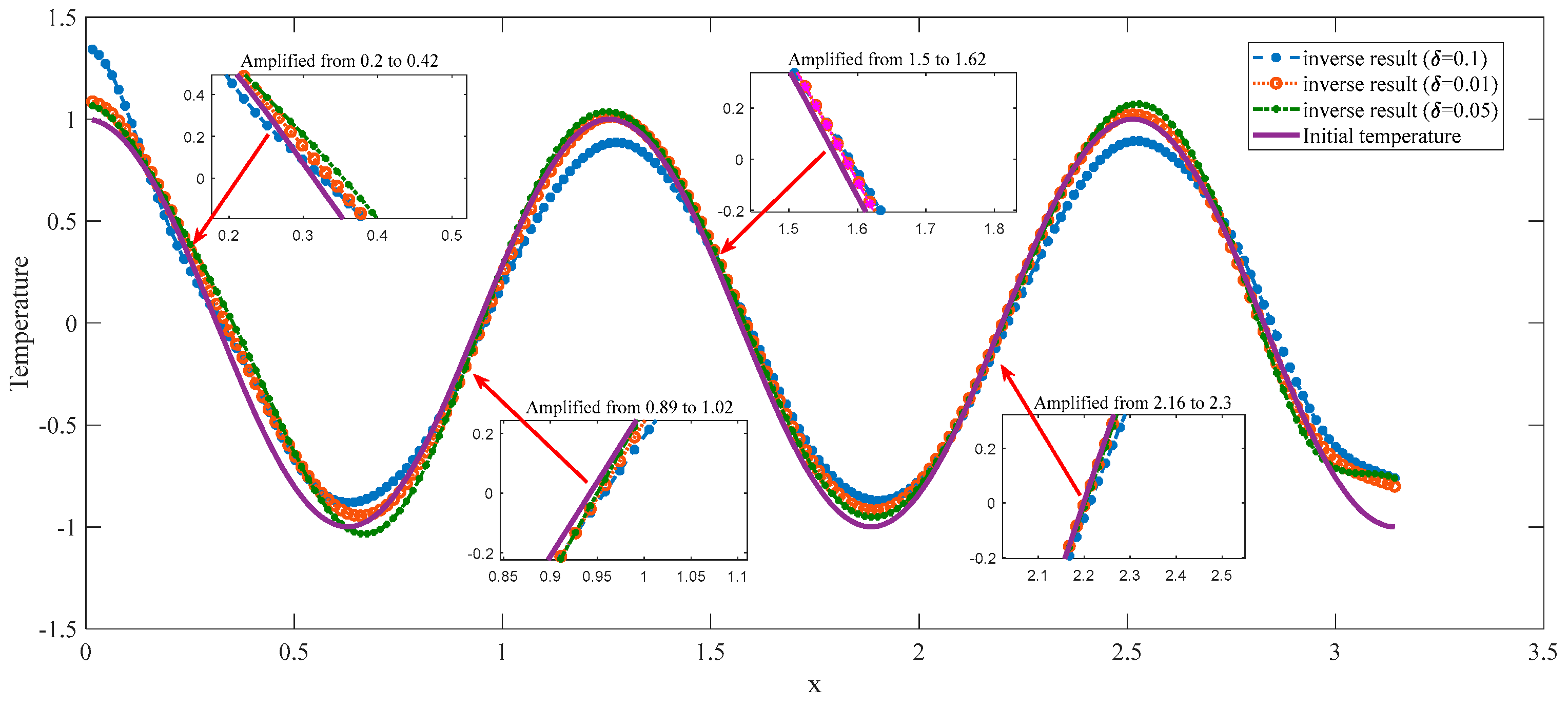
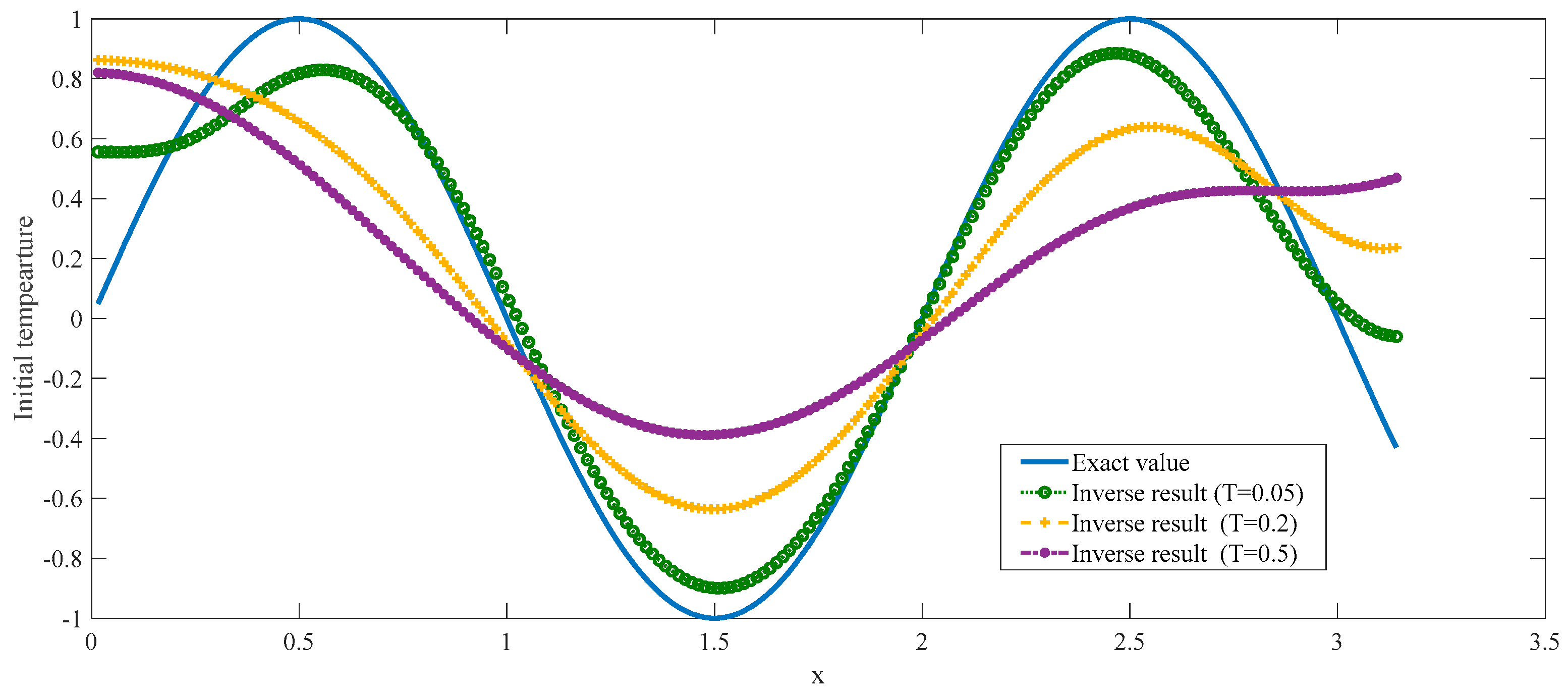
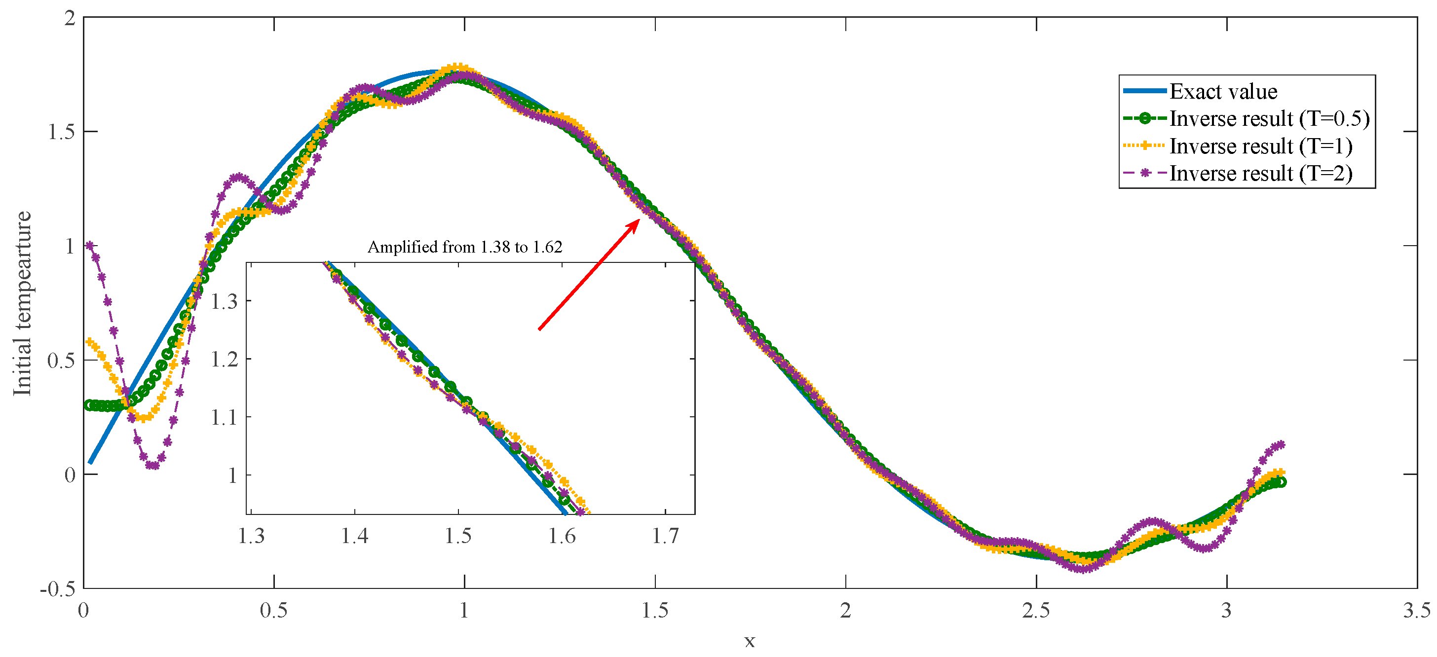
6. The Simulation Experiment

In this section, the numerical simulation experiments of recovering the initial temperature by the truncated regularized optimization scheme are introduced. The key of the regularization method is the selection of the regularization parameter. The main steps of choosing the regularization parameter are shown in the following:

• Step 1: Choose the initial value ${\alpha }_0>0$, error level $\delta >0$, stopping criterion $\epsilon >0$, the maximum number $N_{\max }$ and $k=0$;
• Step 2: Solve the Equations (73) and (74) with respect to $g_{\alpha }^{\delta }$ and $d{g}_{\alpha }^{\delta }/d\alpha$ for $\alpha ={\alpha }_k$;
• Step 3: Compute $G({\alpha }_k)$, $G\prime \left({\alpha }_k\right)$ by Equations (71) and (72) respectively;
• Step 4: Obtain ${\alpha }_{k+1}$ by Equation (80); if $\Vert {\alpha }_{k+1}-{\alpha }_k\Vert \le \epsilon$ or iterative number $k$ reaches the maximum number $N_{\max }$, stop; else go back to step 2.

In this simulation experiment, Example 1 is used to confirm the effectiveness of the improved method of fourth-order convergence. Example 2, Example 3 and Example 4 are used to verify the validity of the truncated regularized optimization scheme.

Example 1.

Consider the following model

$$\{\begin{array}{ll}{u}_t=u_{xx}& (x,t)\in (0,\pi )\times (0,T],\\ {u_x(x,t)|}_{x=0}=0& t\in [0,T],\\ {u_x(x,t)+u|}_{x=\pi }=0& t\in [0,T],\\ u(x,0)=g(x)& x\in (0,\pi ),\end{array}$$

(99)

this is the backward heat conduction problem, which means that the temperature $u(x,T)$ is known to solve $g(x)$. Here $g(x)=\frac{1}{2}\cos x$ and its exact solution is

$$u(x,t)=\frac{1}{2}{e}^{-t}\cos x$$

(100)

Then

$$Kg(x)={\displaystyle {\int }_0^{\pi }f(x,y)g(y)dy},$$

(101)

$$K^{2}g(x)={\displaystyle {\int }_0^{\pi }{\displaystyle {\int }_0^{\pi }f(x,y)f(y,z)g(z)dzdy}}$$

(102)

where $f(x,y)$ is the Kernel function, and its approximate expression is:

$$f(x,y)=\frac{1}{\pi }\left(1+2{\displaystyle \sum _{n=1}^{\infty }\cos nx\cos ny\exp (-n^{2}T)}\right).$$

(103)

The infinite series is approximated by its first 10-items, and the interval $[0,\pi ]$ is divided into $m$ equal parts. We define $x_i=i\cdot \pi /m$, $i=0,1,\dots ,m$, and the integral is calculated by trapezoid formula. According to Equations (101)–(103), the approximate form of Equation (70) is:

$$\alpha g(x)+\frac{{\pi }^2}{{\mathrm{m}}^2}{\displaystyle \sum _{j=0}^m{\overline{b}}_{j}f(x,x_j)}\left[{\displaystyle \sum _{i=0}^m{\overline{b}}_{i}f(x_j,x_i)}g(x_i)\right]=\frac{\pi }{m}{\displaystyle \sum _{i=0}^m{\overline{b}}_{i}f(x,x_i)}{u}^{\delta }(x_i,T),$$

(104)

where ${\overline{b}}_0={\overline{b}}_m=1/2$, ${\overline{b}}_i=1$ for $i=1,2,\dots ,m-1$, and $u^{\delta }(x,T)$ is the measuring data of $u(x,T)$. According to the Equation (6.6), the numerical solution of $g(x)$ can be obtained.

The initial values (${\alpha }_0=0.01$, $\epsilon ={10}^{-8}$, $N_{\max }=50$, $m=100$, $T=0.005$) are chosen in this simulation experiment and the error levels ($\delta =0.001$, $0.005$, $0.01$, $0.015$) are taken to generate the measuring data by

$$u^{\delta }=u+\delta \sin (2x-1).$$

(105)

The regularization parameters are estimated by the improved method of fourth-order convergence, and the results are shown in

Table 1. The comparison of the improved method with other methods (${\alpha }_0=0.01$, $\delta =0.001$).

Algorithm	Iterative Number	${\mathit{\alpha }}^{*}$	$\Vert \mathit{A}\mathit{g}-{\mathit{u}}_{\mathit{\delta }}\Vert /\Vert {\mathit{u}}_{\mathit{\delta }}\Vert$
Newton method [19]	14	2.5396 × 10−4	2.812 × 10−4
Cubic convergent method [22]	12	2.5396 × 10−4	2.812 × 10−4
Chebyshev method [23]	13	2.5396 × 10−4	2.812 × 10−4
Halley method [23]	12	2.5396 × 10−4	2.812 × 10−4
Super-Halley method [23]	11	2.5396 × 10−4	2.812 × 10−4
The improved method	10	2.5396 × 10−4	2.812 × 10−4

and

Table 2. The comparison of the improved method with other methods (${\alpha }_0=0.01$, $\delta =0.005$).

Algorithm	Iterative Number	${\mathit{\alpha }}^{*}$	$\Vert \mathit{A}\mathit{g}-{\mathit{u}}_{\mathit{\delta }}\Vert /\Vert {\mathit{u}}_{\mathit{\delta }}\Vert$
Newton method [19]	12	1.2618 × 10−3	1.4 × 10−3
Cubic convergent method [22]	11	1.2618 × 10−3	1.4 × 10−3
Chebyshev method [23]	11	1.2618 × 10−3	1.4 × 10−3
Halley method [23]	11	1.2618 × 10−3	1.4 × 10−3
Super-Halley method [23]	11	1.2618 × 10−3	1.4 × 10−3
The improved method	9	1.2618 × 10−3	1.4 × 10−3

, respectively. Compared with other methods [19,22,23], the improved method of fourth-order convergence obviously reduces the iterative number under the same accuracy.

Example 2.

Considering the following heat transfer model

$$\{\begin{array}{ll}{u}_t=u_{xx},& (x,t)\in (0,\pi )\times [0,T],\\ {u_x(x,t)|}_{x=0}=0,& t\in [0,T],\\ {u_x(x,t)+h_{1}u|}_{x=\pi }=0,& t\in [0,t_1),\\ {u_x(x,t)+h_{2}u|}_{x=\pi }=0,& t\in [t_1,t_2),\\ {u_x(x,t)+h_{3}u|}_{x=\pi }=0,& t\in [t_2,T],\\ u(x,0)=g(x),& x\in (0,\pi ),\end{array}$$

(106)

where $h_1=1$, $h_2=1/2$, $h_3=1/3$, $t_1=0.002$, $t_2=0.006$, $T=0.01$ and $g(x)=\cos (5x)$.

According to Equation (104), the numerical solution of $g(x)$ can be obtained. The regularization parameter ${\alpha }_i$ ($i=1,2,3$) is obtained by the improved method. Here, we chose the initial values (${\alpha }_0=0.01$, $\epsilon ={10}^{-7}$, $N_{\max }=100$, $m=200$). The measuring data is generated by Equation (105) at time $T=0.01$, in which the error levels are $\delta =0.01$, $\delta =0.05$ and $\delta =0.1$ respectively.

The inverse results recovered by the truncated regularized optimization scheme are shown in Figure 1. In this example, the initial value $g(x)$ is recovered from the measuring data $u^{\delta }(x,T)$ and the inverse results match with the exact values very well.

Example 3.

Consider the problem of Example 2 with the initial value

$$g(x)=u(x,0)=\sin (\pi x)$$

(107)

Similar to Example 2, this example chose the error level $\delta =0.1$ and tests the inverse results for different final times ($T=0.05$, $T=0.2$ and $T=0.5$). The measuring data is generated by Equation (105) at times $T=0.05$, $T=0.2$ and $T=0.5$ respectively. The regularization parameters are decided by the improved method. The inverse results obtained by the Equation (104) are shown in Figure 2.

This example compares the inverse results with the exact values under different final times $T$. From Figure 2, it can be seen that the inverse results become worse with the increase of final time, the reason for which is that the diffusion coefficient $k\left(x\right)=1$ is large. The large diffusion coefficient can lead to rapid changes in the temperature. Furthermore, the diffusion coefficient $k\left(x\right)$ is usually chosen less than 10⁻³ in practice.

Example 4.

Consider the problem of Example 2 with the following initial value

$$g(x)=u(x,0)=\sin (x)+\sin (2x)x\in \left[0,\pi \right].$$

(108)

In this example, we chose the diffusion coefficient $k\left(x\right)=0.01$ and the final times ($T=0.5$, $T=1$ and $T=2$). The measuring data is generated by Equation (105) at time $T=0.5$, $T=1$ and $T=2$ respectively. The inverse results recovered by the truncated regularized optimization scheme are shown in Figure 3 ($\delta =0.01$). The regularization parameters are chosen by the improved method. It can be seen that the inverse results fit the exact values very well under the different final times.

The above three examples show that the inverse method can effectively recover the initial temperature. On the basis of the temperature $g(x)$, the recovering of the whole temperature $u(x,t)$ for $t\in \left(0,T\right)$ can be implemented.

7. Conclusions

This paper considers the backward heat conduction problem, which has a piecewise linear heat transfer coefficient. Firstly, this paper introduces the severely ill-posedness of the backward heat conduction problem (1) and points out that the solution of problem (1) is affected not only by the measuring error but also by the computational error. Secondly, a truncated regularized optimization scheme is developed to solve the problem (1) and the convergence rate of the regularized solution is analyzed. The results of simulation experiments (Example 2, Example 3 and Example 4) show that the inverse values match with the exact values very well. Thirdly, in order to reduce the iterative number, this paper presents an improved method of choosing the regularization parameter, and the fourth-order convergence of this method is proved. Compared with other methods, the results of Example 1 illustrate that the improved method of fourth-order convergence effectively reduces the iterative number.

References

1. Wang, J.G.; Wei, T.; Zhou, Y.B. Tikhonov Regularization Method for a Backward Problem for the Time-Fractional Diffusion Equation. Appl. Math. Model. 2013, 37, 8518–8532. [Google Scholar] [CrossRef]
2. Liu, J.J.; Wang, B.X. Solving the Backward Heat Conduction Problem by Homotopy Analysis Method. Appl. Numer. Math. 2018, 128, 84–97. [Google Scholar] [CrossRef]
3. Milad, K.; Fridoun, M.; Mojtaba, H. On Regularization and Error Estimates for the Backward Heat Conduction Problem with Time-Dependent Thermal Diffusivity Factor. Commun. Nonlinear Sci. 2018, 63, 21–37. [Google Scholar]
4. Tuan, N.H.; Khoa, V.A.; Truong, M.T.N.; Hung, T.T.; Minh, M.N. Application of the Cut-off Projection to Solve a Backward Heat Conduction Problem in a Two-slab Composite System. Inverse Probl. Sci. 2019, 27, 460–483. [Google Scholar] [CrossRef]
5. Tuan, N.H.; Huynh, L.N.; Ngoc, T.B.; Zhou, Y. On a Backward Problem for Nonlinear Fractional Diffusion Equations. Appl. Math. Lett. 2019, 92, 76–84. [Google Scholar] [CrossRef]
6. Chen, Y.W. A Modified Lie-group Shooting Method for Multi-dimensional Backward Heat Conduction Problems under Long Time Span. Int. J. Heat Mass Tran. 2018, 127, 948–960. [Google Scholar] [CrossRef]
7. Chen, Y.W. A Highly Accurate Backward-forward Algorithm for Multi-dimensional Backward Heat Conduction Problems in Fictitious Time Domains. Int. J. Heat Mass Tran. 2018, 120, 499–514. [Google Scholar] [CrossRef]
8. Liu, X.; Qian, Z.M. Backward Problems for Stochastic Differential Equations on the Sierpinski Gasket. Stoch. Proc. Appl. 2018, 10, 3387–3418. [Google Scholar] [CrossRef]
9. Cheng, W.; Ma, Y.J.; Fu, C.L. A Regularization Method for Solving the Radially Symmetric Backward Heat Conduction Problem. Appl. Math. Lett. 2014, 30, 38–43. [Google Scholar] [CrossRef]
10. Su, L.D. A Radial Basis Function (RBF)-Finite Difference (FD) Method for the Backward Heat Conduction Problem. Appl. Math. Comput. 2019, 354, 232–247. [Google Scholar] [CrossRef]
11. Vasil’ev, V.I.; Kardashevskii, A.M. Numerical Solution of the Retrospective Inverse Problem of Heat Conduction with the Help of the Poisson Integral. J. Appl. Ind. Math. 2018, 12, 577–586. [Google Scholar] [CrossRef]
12. Beck, J.V.; Woodbury, K.A. Inverse Heat Conduction Problem: Sensitivity Coefficient Insights, Filter Coefficients, and Intrinsic Verification. Int. J. Heat Mass Tran. 2016, 97, 578–588. [Google Scholar] [CrossRef]
13. Maleki, H.; Safaei, M.R.; Alrashed, A.A.; Kasaeian, A. Flow and Heat Transfer in Non-Newtonian Nanofluids over Porous Surfaces. J. Therm. Anal. Calorim. 2019, 135, 1655–1666. [Google Scholar] [CrossRef]
14. Shahriyar, G.H.; Faramarz, T.; Masood, S. Analytical Solution of Steady State Heat Conduction Equations in Irregular Domains with Various BCs by Use of Schwarz-Christoffel Conformal Mapping. Thermal Sci. Eng. Progress 2019, 11, 8–18. [Google Scholar]
15. Cheng, Y.K.; Chih, Y.L.; Wei, Y.; Chein, S.L.; Chia, M.F. A Novel Space–Time Meshless Method for Solving the Backward Heat Conduction Problem. Int. J. Heat Mass Tran. 2019, 130, 109–122. [Google Scholar]
16. Chen, D.H.; Hofmann, B.; Zou, J. Regularization and Convergence for Ill-posed Backward Evolution Equations in Banach Spaces. J. Differ. Equat. 2018, 265, 3533–3566. [Google Scholar] [CrossRef]
17. Yu, Y.; Luo, X.C.; Liu, Q. Model Predictive Control of a Dynamic Nonlinear PDE System with Application to Continuous Casting. J. Process Contr. 2018, 65, 41–55. [Google Scholar] [CrossRef]
18. Wang, Y.; Luo, X.; Zhang, F.; Wang, S. GPU-based Model Predictive Control for Continuous Casting Spray Cooling Control System Using Particle Swarm Optimization. Control Eng. Pract. 2019, 84, 349–364. [Google Scholar] [CrossRef]
19. Hou, R.R. Selection of Regularization Parameter for L1-regularized Damage Detection. J. Sound Vib. 2018, 423, 141–160. [Google Scholar] [CrossRef]
20. Park, Y.; Reichel, L.; Rodriguez, G.; Yu, X. Parameter Determination for Tikhonov Regularization Problems in General Form. J. Comput. Appl. Math. 2018, 343, 12–25. [Google Scholar] [CrossRef]
21. Reddy, G.D. A Class of Parameter Choice Rules for Stationary Iterated Weighted Tikhonov Regularization Scheme. Appl. Math. Comput. 2019, 347, 464–476. [Google Scholar] [CrossRef]
22. Neggal, B.; Boussetila, N.; Rebbani, F. Projected Tikhonov Regularization Method for Fredholm Integral Equations of The First Kind. J. Inequal. Appl. 2016, 195, 1–21. [Google Scholar]
23. Zou, Y.K.; Wang, L.J.; Zhang, R. Cubically Convergent Methods for Selecting the Regularization Parameters in Linear Inverse Problems. J. Math. Anal. Appl. 2009, 356, 355–362. [Google Scholar] [CrossRef]
24. Chun, C.B. Some Fourth-order Iterative Method for Solving Nonlinear Equations. Appl. Math. Comput. 2008, 195, 454–459. [Google Scholar] [CrossRef]
25. Li, H.; Liu, J.J. Solution of Backward Heat Problem by Morozov Discrepancy Principle and Conditional Stability. Numer. Math. J. Chin. Univ. 2005, 14, 180–192. [Google Scholar]
Figure 1. Recovery of u ( x , 0 ) from the measuring data u δ ( x , T ) with different δ .
Mathematics 07 00388 g001
Figure 2. Recovery of u ( x , 0 ) from exact u ( x , T ) with different T .
Mathematics 07 00388 g002
Figure 3. Recovery of u ( x , 0 ) from exact u ( x , T ) with different T .
Mathematics 07 00388 g003