Computing μ-Values for Real and Mixed μ Problems

Abstract

In various modern linear control systems, a common practice is to make use of control in the feedback loops which act as an important tool for linear feedback systems. Stability and instability analysis of a linear feedback system give the measure of perturbed system to be singular and non-singular. The main objective of this article is to discuss numerical computation of the $\mu$-values bounds by using low ranked ordinary differential equations based technique. Numerical computations illustrate the behavior of the method and the spectrum of operators are then numerically analyzed.

1. Introduction

In system theory, $\mu$-value known as structured singular value (SSV) is a well-defined tool, first introduced by Doyle [1]. It is used to analyze the robustness of linear feedback systems when they are subject to uncertainties, particularly structured uncertainties. The $\mu$-value tool has vast applications in control engineering, for instance, for the analysis of controller of an unstable system, the MIMO margins by using $\mu$ and for the space shuttle robustness analysis [2]. For more applications, we refer [3,4] and the references therein.

The numerical approximation of SSV appears as NP-hard problem [5,6]. The computation of the upper bounds of $\mu$-values is a hard problem; in fact, the NP-hard is in nature when only real uncertainties appear [7].

The power method [3,8] is used to approximate the lower bounds of $\mu$-values when only pure complex uncertainties are under consideration. This is a seemingly robust numerical method due to the fact that it depends solely on matrix-vector products. The power method is easy to apply only when mixed real perturbations and complex perturbations are taken into account [9,10,11]. This method resembles a mixture of power techniques used for the computation of eigenvalues and singular values of the constant matrices. This method also prove that $\mu$-values act as an equilibrium point of the power technique. The power method fails to numerically compute the lower bounds of $\mu$-values only when pure real uncertainties are under discussion. We refer to [12,13,14,15,16,17,18,19,20] and references therein for a comprehensive study of the numerical algorithms to compute numerically the bounds of $\mu$-values from below.

An approximation of bounds of $\mu$-values involve fundamental difficulties when one considers pure real uncertainties because the real $\mu$-values might be discontinuous function of the given problem data [21,22]. Thus the available algorithms [13,14,15,19] to deal such problems have a computational cost which has exponential growth in nature. The idea of regularization to such a problem helps to reduce computational cost by making use of the mixed real/complex power iteration.

In this article, we use an iterative method [23] in order to numerically compute the $\mu$-values bounds from below for a set of constant matrices generated randomly. The idea is based on a two level algorithm described in a great detail in [23]. The inner algorithm provides basis to develop a gradient system of ordinary differential equations (ODEs) and eventually solves this system by making use of extremizers of structured spectral-value sets. On the other hand, The outer algorithm helps to adjust the small positive parameter which acts as valid perturbation $ϵ>0$, when making use of fast Newton’s iteration.

This paper is organized as follows: In Section 2 we provide the basic definitions of pseudo-spectra and structured singular values. In Section 3 we give the reformulation of the definition of structured singular values. Section 4 of this article contains the computation of pseudo-spectra, where in Section 5 we explain how the computation of structured singular values can be addressed by making use of an inner-outer algorithm. In the outer algorithm, we determine a small perturbation level $ϵ$ while in inner algorithm we determines a local extremizer of the structured spectral value set. Section 6 refers to numerical experiments to compare the lower bounds of SSV obtained with algorithm [23] to those obtained with MATLAB function mussv. Section 7 summarizes our conclusions.

2. Preliminaries

Definition 1.

The uncertainties in terms of mixed real and complex scalar blocks are denoted by ${\mathbb{B}}_{rc}$ and defined by

$${\mathbb{B}}_{rc}:=\{Diag({\delta }_1{I}_1,{\delta }_2{I}_2,\dots ,{\delta }_s{I}_s;{\delta }_{s+1}{I}_{s+1},{\delta }_{s+2}{I}_{s+2},\dots ,{\delta }_{s+n}{I}_{s+n}):{\delta }_i\in \mathbb{R}\forall i=1:s,{\delta }_{s+j}\in \mathbb{C}\forall j=1:n\}.$$

(1)

Definition 2.

The set of block diagonal matrices in terms of pure real scalar blocks is denoted by ${\mathbb{B}}_r$ and defined by

$${\mathbb{B}}_r:=\{Diag({\delta }_1{I}_1,{\delta }_2{I}_2,\dots ,{\delta }_s{I}_s):{\delta }_i\in \mathbb{R}\forall i=1:s\}.$$

(2)

Definition 3.

The set of uncertainties in terms of pure full complex blocks are denoted by ${\mathbb{B}}_f$, defined as

$${\mathbb{B}}_f:=\{Diag({\Delta }_1,{\Delta }_2,\dots ,{\Delta }_F):{\Delta }_j\in {\mathbb{C}}^{m_j,m_j}\forall j=1:F\}.$$

(3)

Definition 4.

The uncertainties in terms of blocks consist of r repeated real scalar blocks and F square full complex blocks are denoted by ${\mathbb{B}}_R$ and defined as follows

$${\mathbb{B}}_R:=\{Diag({\delta }_1{I}_{r_1},{\delta }_2{I}_{r_2},\dots ,{\delta }_s{I}_{r_S},{\Delta }_1,{\Delta }_2,\dots ,{\Delta }_F):{\delta }_i\in \mathbb{R},{\Delta }_j\in {\mathbb{C}}^{m_j,m_j}\}.$$

(4)

Definition 5.

The block diagonal operators entirely consist of S repeated complex scalar blocks and F square full complex blocks are denoted by ${\widehat{\mathbb{B}}}_R$ and defined as

$${\widehat{\mathbb{B}}}_R:=\{\mathrm{Diag}({\delta }_1{I}_1,{\delta }_2{I}_2,\dots ,{\delta }_S{I}_S,{\Delta }_1,{\Delta }_2,\dots ,{\Delta }_F):{\delta }_i\in \mathbb{C},{\Delta }_j\in {\mathbb{C}}^{m_j,m_j}\}.$$

(5)

Definition 6.

The spectrum of a square complex valued matrix $M\in {\mathbb{C}}^{n,n}$ is represented by $\mathsf{\Lambda }(M)$ and mathematically defined as

$$\mathsf{\Lambda }(M)=\{\lambda \in \mathbb{C}:det\left(\lambda I-M\right)=0\}.$$

(6)

Definition 7.

The pseudo-spectrum of a n-dimensional complex valued operator is represented by ${\mathsf{\Lambda }}_{ϵ}(M)$ and defined as:

$${\mathsf{\Lambda }}_{ϵ}(M)=\left\{\lambda \in \mathbb{C}:\parallel {\left(\lambda I-M\right)}^{-1}\parallel \ge \frac{1}{ϵ}\right\}.$$

(7)

Definition 8.

The μ-value of $M\in {\mathbb{C}}^{n\times n}$ underlying block diagonal operator $\mathbb{B}$ is mathematically denoted by ${\mu }_{{\mathbb{B}}_R}(M)$ and defined as follows

$$\begin{array}{cc}\hfill {\mu }_{{\mathbb{B}}_R}(M)& :=\left\{\begin{array}{ccc}0,\hfill & if\hfill & |I-M\Delta |\ne 0,\forall \Delta \in {\mathbb{B}}_R,\hfill \\ {\displaystyle \frac{1}{min\{||\Delta |{|}_2:|I-M\Delta |=0,\Delta \in {\mathbb{B}}_R\}}},\hfill & \hfill & otherwise.\hfill \end{array}\right.\hfill \end{array}$$

(8)

3. Reformulation of $\mathbf{\mu }$-Values

In this section we give the reformulation of μ-values based on structured spectral value sets [24]. The reformulation of μ-values allows us to construct an optimization problem in order to maximize the spectrum of the perturbed system.

Definition 9.

The ϵ-spectral valued set of an n-dimensional complex operator underlying a small positive real parameter $ϵ>0$ is mathematically denoted by ${\Delta }_{ϵ}^{{\mathbb{B}}_R}(M)$ and defined as:

$${\mathsf{\Lambda }}_{ϵ}^{{\mathbb{B}}_R}(M):=\{\lambda \in \mathsf{\Lambda }(ϵM\Delta ),\Delta \in {\mathbb{B}}_R{,\left|\right|\Delta \left|\right|}_2\le 1\},$$

(9)

where the quantity $\mathsf{\Lambda }(ϵM\Delta )$ represent the spectrum of an operator $(ϵM\Delta )$ while ${\left|\right|\Delta \left|\right|}_2$ represents the greatest singular value of an operator $\Delta \in {\mathbb{B}}_R$.

Definition 10.

For a given n-dimensional complex operator M and an underlying perturbation in the form of $\mathbb{B}$, the spectral value set is represented by ${\mathsf{\Sigma }}_{ϵ}^{{\mathbb{B}}_R}(M)$ and is defined as the following

$${\mathsf{\Sigma }}_{ϵ}^{{\mathbb{B}}_R}(M):=\{\eta =1-\lambda :\lambda \in {\mathsf{\Lambda }}_{ϵ}^{{\mathbb{B}}_R}(M)\}.$$

(10)

Definitions 9 and 10 make it possible to formulate again μ-value as a maximization problem.

Definition 11.

For $M\in {\mathbb{C}}^{n\times n}$ and a set of pure complex uncertainties ${\widehat{\mathbb{B}}}_R$, μ-value is defined as the following

$$\begin{array}{c}\hfill {\mu }_{{\widehat{\mathbb{B}}}_R}(M)={\displaystyle \frac{1}{arg\{max|\lambda |=1,\lambda \in {\mathsf{\Lambda }}_{ϵ}^{{\mathbb{B}}_R}(M)\}}},\end{array}$$

(11)

with ${\widehat{\mathbb{B}}}_R=\{\mathit{Diag}({\delta }_1{I}_{c_1},{\delta }_2{I}_{c_2},\dots ,{\delta }_S{I}_{c_S},{\Delta }_1,{\Delta }_2,\dots ,{\Delta }_F):{\delta }_i\in \mathbb{C},{\Delta }_j\in {\mathbb{C}}^{m_j,m_j}\}$.

4. Pseudospectra of Square Matrices

In this section, the pseudospectra for matrices are under consideration. For this purpose we make use of the software package EigTool [25]. EigTool is routinely used to plot the unstructured pseudospectra of the matrices under consideration. Figure 1 and Figure 2 show the graphical representation of the pseudospectrum of 6-dimensional and 4-dimensional real valued matrices.

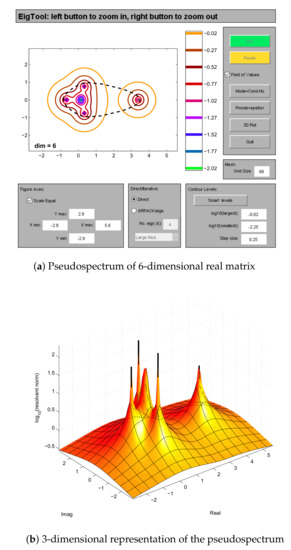
Figure 1. MATLAB interface for computing pseudospectrum.

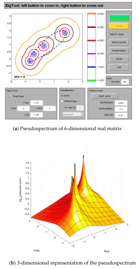
Figure 2. MATLAB interface for computing pseudospectrum.

We consider a six dimensional real valued matrix M as

$$M=\left[\begin{array}{cccccc}0.8147& 0.2785& 0.9572& 0.7922& 0.6787& 0.7060\\ 0.9058& 0.5469& 0.4854& 0.9595& 0.7577& 0.0318\\ 0.1270& 0.9575& 0.8003& 0.6557& 0.7431& 0.2769\\ 0.9134& 0.9649& 0.1419& 0.0357& 0.3922& 0.0462\\ 0.6324& 0.1576& 0.4218& 0.8491& 0.6555& 0.0971\\ 0.0975& 0.9706& 0.9157& 0.9340& 0.1712& 0.8235\end{array}\right].$$

Next, we consider a four dimensional complex valued matrix M as

$$M=\left[\begin{array}{cccc}0.2374+0.9338i& 0.1048+0.4876i& 0.6035+0.0372i& 0.7581+0.6099i\\ 0.5309+0.1875i& 0.1123+0.7690i& 0.9644+0.6733i& 0.4326+0.0594i\\ 0.0915+0.2662i& 0.7844+0.3960i& 0.4325+0.4296i& 0.6555+0.3158i\\ 0.4053+0.7978i& 0.2916+0.2729i& 0.6948+0.4517i& 0.1098+0.7727i\end{array}\right].$$

and compute pseudo-spectra with EigTool.

5. Proposed Methodology

In this section, the main objective is to discuss the optimization problem as mentioned in Definition 11, we make use of a numerical approach which is based on low-ranked ordinary differential equations. The numerical method is composed of a two-level algorithm, the inner algorithm and an outer algorithm. In this Section, we first discuss the inner-algorithm which shows how to give a theoretical construction to the system of ordinary differential equations. Secondly, we discuss how to deal with such systems mathematically. Next, we discuss the outer algorithm, which helps to modify the small positive real parameter $ϵ>0$. The outer algorithm is based on Newton’s iteration for approximating the roots of non-linear equations. The outer-algorithm computes an exact derivative of an extremizer say, $\Delta (ϵ)$ for $\Delta \in \mathbb{B}$ and $ϵ>0$. Complete details of the numerical method under consideration are given in [23,24]. Finally, we discuss the computation of an extremizer. For this purpose, we approximate the derivative of an eigenvalue matrix $\mathsf{\Lambda }(p)$ of a smooth matrix family say $A(p)$ for some fixed parameter p.

5.1. Inner-Algorithm

5.1.1. The Basic Theory

Consider some smooth matrix family $A(p)\in {\mathbb{C}}^{n,n}$ for a small parameter p. Let $\mathsf{\Lambda }(p)\in {\mathbb{C}}^{n,n}$ and $X(p)\in {\mathbb{C}}^{n,n}$ be the eigenvalue and eigenvector matrices corresponding to $A(p)$. In matrix form

$$A(p)X(p)=X(p)\mathsf{\Lambda }(p).$$

(12)

In Equation (12), computation of eigenvector matrix $X(p)$ is not unique unless all of the eigenvectors remain fixed. For distinct eigenvalues all of the eigenvectors are computed up to a constant multiplier.

The theory of computing $X(p)$ is extended if eigenvalue derivatives are repeated while the second order derivatives of eigenvalues remain distinct. This theory is further generalized to complex-valued and Hermitian matrix.

Here and hereafter the symbol $(\prime )$ denotes the derivative while we write $A=A(p)$, that is, we omit the dependency on p. By differentiating Equation (12) we get,

$$A^{{}^{\prime }}X+A{X}^{{}^{\prime }}=X^{{}^{\prime }}\mathsf{\Lambda }+X{\mathsf{\Lambda }}^{{}^{\prime }},$$

or

$$A^{{}^{\prime }}X-X{\mathsf{\Lambda }}^{{}^{\prime }}=-A{X}^{{}^{\prime }}+X^{{}^{\prime }}\mathsf{\Lambda }.$$

(13)

Our goal is to determine ${\mathsf{\Lambda }}^{{}^{\prime }}$, the derivative of eigenvalues matrix. For this purpose, we multiply Equation (13) with $X^{-1}$ throughout to have,

$$X^{-1}{A}^{{}^{\prime }}X-X^{-1}X{\mathsf{\Lambda }}^{{}^{\prime }}=-X^{-1}A{X}^{{}^{\prime }}+X^{-1}{X}^{{}^{\prime }}\mathsf{\Lambda }.$$

Since $X^{-1}X=I$, this implies:

$$X^{-1}{A}^{{}^{\prime }}X-{\mathsf{\Lambda }}^{{}^{\prime }}=-X^{-1}A{X}^{{}^{\prime }}+X^{-1}{X}^{{}^{\prime }}\mathsf{\Lambda },$$

(14)

let $L=X^{-1}{X}^{{}^{\prime }}$, we find

$$X^{{}^{\prime }}=XL,$$

thus Equation (14) gives:

$$X^{-1}{A}^{{}^{\prime }}X-{\mathsf{\Lambda }}^{{}^{\prime }}=-X^{-1}AXL+L\mathsf{\Lambda },$$

or

$$X^{-1}{A}^{{}^{\prime }}X-{\mathsf{\Lambda }}^{{}^{\prime }}=-X^{-1}X\mathsf{\Lambda }L+L\mathsf{\Lambda }.$$

Therefore,

$$X^{-1}{A}^{{}^{\prime }}X-{\mathsf{\Lambda }}^{{}^{\prime }}=-\mathsf{\Lambda }L+L\mathsf{\Lambda }.$$

(15)

Finally, this gives the required result for the computation of the derivative of spectrum of matrix valued function $A(p)$ as follows

$$X^{-1}{A}^{{}^{\prime }}X-{\mathsf{\Lambda }}^{{}^{\prime }}=0,\mathrm{or}{\mathsf{\Lambda }}^{{}^{\prime }}=X^{-1}{A}^{{}^{\prime }}X.$$

5.1.2. Approximation of Extremizers

A matrix valued function $\Delta \in \mathbb{B}$ having the largest eigenvalue bounded above by 1 and the matrix valued function $(I-ϵM\Delta )$ having a smallest eigenvalue which minimizes the modulus of structured spectral value set, ${\sum }_{ϵ}^{\mathbb{B}}(M)$ is known as an extremizer. The following theorem computes an extremizer for a chosen smallest complex number belonging to the set ${\sum }_{ϵ}^{\mathbb{B}}(M)$.

Theorem 1 ([23]).

For a perturbation $\Delta \in \mathbb{B}$ having the block diagonal structure

$$\Delta =\{Diag({\delta }_1{I}_1,\cdots {\delta }_{s^{{}^{\prime }}}{I}_{s^{{}^{\prime }}},{\delta }_{s^{{}^{\prime }}+1}{I}_{s^{{}^{\prime }}+1},\cdots {\delta }_S{I}_S;{\Delta }_1,\cdots ,{\Delta }_F)\},$$

with ${\parallel \Delta \parallel }_2=1,$ acts as a local extremizer of structured spectral value set. For a simple smallest eigenvalue $\lambda =\left|\lambda \right|e^{\iota \theta },\theta \in \mathbb{R}$ of matrix valued function $(I-ϵM\Delta )$ having right and left eigenvetors x and y scaled as $S=e^{\iota \theta }{y}^{*}x$ and let $z=M^{*}y$. The non-degeneracy conditions

$$z_k^{*}{x}_k\ne 0, \forall =1:S^{{}^{\prime }}$$

$$Re(z_k^{*}{x}_k)\ne 0, \forall =1:S^{{}^{\prime }}+1:S$$

$$and\left|\right|z_{s+h}\left|\right|.\left|\right|x_{s+h}\left|\right|\ne 0, \forall h=1:F,$$

hold. Then magnitude of each complex scalar${\delta }_i\forall i=1:s$appears to be exactly equal to 1 while each full block possesses a unit 2-norm.

Proof. 

For proof we refer to [23]. □

5.1.3. Gradient System of ODEs

The gradient system of ODEs for an admissible perturbation $\Delta \in \mathbb{B}$ to approximate a local extremizer of smallest eigenvalue $\lambda =\left|\lambda \right|{ϵ}^{i\theta }$, is obtained as,

$$\dot{{\delta }_i}={\nu }_i(x_i^{*}{z}_i-Re(x_i^{*}{z}_i\overline{{\delta }_i}){\delta }_i); i=1:s^{{}^{\prime }}$$

$$\dot{{\delta }_l}=sign(Re(z_l^{*}{x}_l)){\Psi }_{(-1,1)}({\delta }_l); l=s^{{}^{\prime }}+1:s$$

$$\dot{{\Delta }_j}={\nu }_j(z_{s+j}{x}_{s+j}^{*}-Re⟨{\Delta }_j;z_{s+j}{x}_{s+j}^{*}⟩); j=1:F,$$

where ${\delta }_i\in \mathbb{C},\forall i=1:s^{{}^{\prime }},{\delta }_l\in \mathbb{R}$ for $l=s^{{}^{\prime }}+1$ and ${\Psi }_{(-1,1)}$ is a characteristic function. For a further discussion on the construction of gradient system of ODEs in above equations, we refer to [23].

5.2. Outer-Algorithm

In an outer-algorithm the main aim is to vary $ϵ>0$, the perturbation level, by means of a fast Newton’s iteration. In turn, $1/ϵ$ will provide the approximation of lower bound of μ-value.

We make use of fast Newton’s iteration in order to solve a problem

$$|\lambda (ϵ)|=1,ϵ>0.$$

(16)

In order to solve Equation (16), we need to compute

$$\frac{d}{dϵ}\left(|\lambda (ϵ)|\right),$$

the derivative.

The following Theorem 2 helps us to compute $\frac{d}{dϵ}(|\lambda (ϵ)|)$, when $|\lambda (ϵ)|$ is simple and $\Delta (0)$, $\lambda (0)$ are assumed to remains smooth in the neighboring region of perturbation level $ϵ>0$.

Theorem 2 ([23]).

Consider matrix valued function $\Delta \in \mathbb{B}$. Let x and y as a function of perturbation level $ϵ>0$ acts as right and left eigenvectors of matrix valued function $(ϵM\Delta )$. Consider the scaling of these vector accordingly to Theorem 1. Let $z=M^{*}y$ and assume that non-degenracy conclusions as discussed in Theorem 1 yield then

$${\displaystyle \frac{d}{dϵ}}(|\lambda (ϵ)|)={\displaystyle \frac{1}{|y({ϵ}^{*})x(ϵ)|}}\left(\sum _{i=1}^s|z_i{(ϵ)}^{*}{x}_i(ϵ)|+\sum _{j=1}^F\left|\right|z_{s+j}(ϵ)\left|\right|.\left|\right|y_{s+j}(ϵ)\left|\right|\right)>0.$$

(17)

Proof. 

For proof we refer to [23]. □

Remark 1.

Choice of suitable initial value matrix and initial perturbation level: For a suitable choice of the initial value matrix ${\Delta }_0$ and an initial perturbation level ${ϵ}_0$, we refer to [23].

6. Numerical Computation

In this section, we present numerical results for both lower and upper bounds of μ-values for randomly generated matrices in MATLAB (R2018a, MathWorks, Natick, MA, USA). The numerical computation of the lower bounds of structured singular values with the help of Nalgo, show the tighter results for the μ-values lower bounds computed by means of well-known MATLAB routine mussv. In each experiment the admissible uncertainties ∇ and E are computed with the help of mussv and Nalgo [23] respectively.

Example 1.

First we consider a six dimensional real valued matrix M

$$M=\left[\begin{array}{cccccc}0.8147& 0.2785& 0.9572& 0.7922& 0.6787& 0.7060\\ 0.9058& 0.5469& 0.4854& 0.9595& 0.7577& 0.0318\\ 0.1270& 0.9575& 0.8003& 0.6557& 0.7431& 0.2769\\ 0.9134& 0.9649& 0.1419& 0.0357& 0.3922& 0.0462\\ 0.6324& 0.1576& 0.4218& 0.8491& 0.6555& 0.0971\\ 0.0975& 0.9706& 0.9157& 0.9340& 0.1712& 0.8235\end{array}\right].$$

We choose block uncertainties $\mathcal{B}=Diag\{{\Delta }_1:{\Delta }_1\in {\mathbb{C}}^{6,6}\}.$ The admissible uncertainty ∇ is given as below

$$\nabla =\left[\begin{array}{cccccc}0.0615& 0.0421& 0.0607& 0.0427& 0.0479& 0.0453\\ 0.0692& 0.0473& 0.0683& 0.0480& 0.0539& 0.0509\\ 0.0545& 0.0373& 0.0538& 0.0378& 0.0425& 0.0401\\ 0.0628& 0.0430& 0.0619& 0.0436& 0.0489& 0.0462\\ 0.0609& 0.0417& 0.0601& 0.0423& 0.0475& 0.0448\\ 0.0727& 0.0497& 0.0717& 0.0504& 0.0566& 0.0535\end{array}\right],$$

with ${\parallel \nabla \parallel }_2=0.3157.$ The main drawback with mussv is that it does not compute the unit 2-norm of each block of admissible perturbation Δ and by this way it loose the optimality condition. The optimality condition requires that: not only the admissible perturbation Δ should possess unit 2-norm but each of its block also possesses a unit 2-norm.

The approximated lower bound of μ-value is $3.1677$. Moreover, by using the algorithm [23], the admissible perturbation E is obtained as

$$E=\left[\begin{array}{cccccc}0.1813& 0.1691& 0.1611& 0.1079& 0.1286& 0.1718\\ 0.2059& 0.1921& 0.1830& 0.1225& 0.1460& 0.1952\\ 0.2140& 0.1997& 0.1902& 0.1273& 0.1518& 0.2028\\ 0.2397& 0.2237& 0.2131& 0.1427& 0.1700& 0.2273\\ 0.1844& 0.1721& 0.1639& 0.1097& 0.1308& 0.1748\\ 0.1179& 0.1100& 0.1048& 0.0702& 0.0836& 0.1118\end{array}\right],$$

with ${\parallel E\parallel }_2=1.$ The algorithm [23] computes the unit 2-norm of admissible perturbation E. It does not violate the optimality condition and hence computes the unit 2-norm against each block of E. The lower bound approximation is $3.5693$ which is a much better approximation than the one computed numerically.

If instead of full complex blocks, one chose the uncertainties to be repeated as complex blocks, then the mussv routine will not compute the desired admissible perturbations such that each repeated complex block possesses a unit 2-norm. On the hand, Nalgo computes each repeated complex block in such a way that not only the admissible perturbation possesses a unit 2-norm but each individual block also has a largest singular value to be exactly equal to 1.

In Table 1, we present the comparison for the lower and upper bounds of μ-value approximated numerically with the help of mussv and an efficient numerical algorithm [23] for matrix M in Example 1. The first column presents the size of an operator M, where the second, third and fourth columns represent the approximations towards both upper and lower bounds which are computed numerically and the lower bounds ${\mu }_l^{\mathrm{Nalgo}}$ computed with the help of [23] respectively.

Table 1. Computation of bounds of μ-values.

n	${\mathit{\mu }}_{\mathit{u}}^{\mathbf{mussv}}$	${\mathit{\mu }}_{\mathit{l}}^{\mathbf{mussv}}$	${\mathit{\mu }}_{\mathit{l}}^{\mathbf{Nalgo}}$
6	2.6579	2.6504	2.8158
6	2.9758	2.9630	2.4962
6	2.9778	2.9654	2.9835
6	2.7771	2.7696	2.7611
6	2.8483	2.8464	2.5008

Example 2.

We consider a four dimensional complex valued matrix M

$$M=\left[\begin{array}{cccc}0.2374+0.9338i& 0.1048+0.4876i& 0.6035+0.0372i& 0.7581+0.6099i\\ 0.5309+0.1875i& 0.1123+0.7690i& 0.9644+0.6733i& 0.4326+0.0594i\\ 0.0915+0.2662i& 0.7844+0.3960i& 0.4325+0.4296i& 0.6555+0.3158i\\ 0.4053+0.7978i& 0.2916+0.2729i& 0.6948+0.4517i& 0.1098+0.7727i\end{array}\right].$$

We choose the perturbation set $\mathcal{B}=Diag\{{\Delta }_1:{\Delta }_1\in {\mathbb{C}}^{4,4}\}.$ The perturbation set contains only pure complex full blocks. The admissible perturbation ∇ is obtained as

$$\nabla =\left[\begin{array}{cccc}0.0520-0.0934i& 0.0694-0.1567i& 0.1073-0.0797i& 0.0794-0.1041i\\ 0.0371-0.0539i& 0.0513-0.0914i& 0.0699-0.0424i& 0.0543-0.0588i\\ 0.0144-0.0590i& 0.0144-0.0963i& 0.0468-0.0598i& 0.0278-0.0690i\\ 0.0352-0.0752i& 0.0452-0.1252i& 0.0788-0.0676i& 0.0558-0.0850i\end{array}\right],$$

with ${\parallel \nabla \parallel }_2=0.4176.$

The numerical result for the lower bound of μ-value is $2.3948$. Moreover by using the algorithm [23], the admissible perturbation E is obtained as

$$E=\left[\begin{array}{cccc}0.1332-0.2201i& 0.1503-0.1958i& 0.1388-0.1551i& 0.0912-0.2321i\\ 0.1095-0.1970i& 0.1253-0.1763i& 0.1165-0.1403i& 0.0723-0.2062i\\ 0.2603-0.1604i& 0.2652-0.1255i& 0.2309-0.0887i& 0.2224-0.1960i\\ 0.1974-0.1872i& 0.2081-0.1577i& 0.1849-0.1194i& 0.1579-0.2113i\end{array}\right],$$

with ${\parallel E\parallel }_2=1.$ The lower bound approximation is $2.6983$. If instead of full complex blocks, one choose the uncertainties to be repeated complex blocks then the mussv routine will not compute the desired admissible perturbations such that each repeated complex block possesses a unit 2-norm. On the other hand, Nalgo computes each repeated complex block in a such a way that not only the admissible perturbation possesses a unit 2-norm but each individual block also have a largest singular value to be exactly equal to 1.

Table 2 represents the comparison of the μ-values approximated numerically with the mussv routine and an iterative method [23] for matrix M taken in Example 2. In the very first column, we present the size of the matrix M. In the second column, the upper bounds of μ-values are presented while lower bounds are presented in the third and fourth columns, respectively.

Table 2. Computation of bounds of μ-values.

n	${\mathit{\mu }}_{\mathit{u}}^{\mathbf{mussv}}$	${\mathit{\mu }}_{\mathit{l}}^{\mathbf{mussv}}$	${\mathit{\mu }}_{\mathit{l}}^{\mathbf{Nalgo}}$
6	2.7392	2.7379	2.7885
6	1.5106	0.0000	1.5027
6	3.1980	3.1945	3.0202
6	0.7588	0.0000	1.3416
6	3.0524	3.0515	2.9231

In Figure 3, we show numerical approximation of bounds of μ-values for matrix valued function $M({\omega }_i)$ at various frequencies ${\omega }_i,\forall i=1:5$. In Cases 1–6, the matrix valued functions $M({\omega }_i)$ are obtained in MATLAB by using the “rand” command. The geometrical interpretation of μ-values bounds show the comparison of μ-values bounds computed numerically from below with the help of Nalgo and the one computed with the help of mussv. The frequency response ${\omega }_i$ is the quantitative measure of output of $M-\Delta$ system.

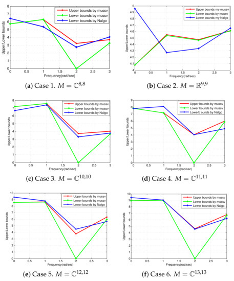
Figure 3. Numerical approximation of bounds of μ-values at different frequency response.

7. Conclusions

In this article, we presented numerical computation of lower and upper bounds of μ-values a well-known mathematical quantity in control. The μ-values discuss robustness and performance of linear feedback systems in control and their bounds examine stability analysis of such systems. The numerical computations show that the attained results for μ-values bounds from below are more appropriate than those obtained by MATLAB function mussv. The EigTool discussed the geometrical interpretation of the pseudo-spectrum of the family of matrices.

References

- Doyle, J. Analysis of feedback systems with structured uncertainties. IEE Proc. D Control Theory Appl. 1982, 129, 242–250. [Google Scholar] [CrossRef]
- Balas, G.J.; Doyle, J.C.; Glover, K.; Packard, A.; Smith, R. μ-Analysis and Synthesis Toolbox User’S Guide; The Mathworks Inc.: Natick, MA, USA, 1995. [Google Scholar]
- Packard, A.; Doyle, J. The complex structured singular value. Automatica 1993, 29, 71–109. [Google Scholar] [CrossRef]
- Ferreres, G. A Practical Approach to Robustness Analysis with Aeronautical Applications; Springer Science & Business Media: Berlin, Germany, 1999. [Google Scholar]
- Braatz, R.P.; Young, P.M.; Doyle, J.C.; Morari, M. Computational complexity of mu-calculation. IEEE Trans. Autom. Control 1994, 39, 1000–1002. [Google Scholar] [CrossRef]
- Demmel, J. The componentwise distance to the nearest singular matrix. SIAM J. Matrix Anal. Appl. 1992, 13, 10–19. [Google Scholar] [CrossRef]
- Fu, M. The real structured singular value is hardly approximable. IEEE Trans. Autom. Control 1997, 42, 1286–1288. [Google Scholar]
- Packard, A.; Fan, M.K.H.; Doyle, J. A power method for the structured singular value. In Proceedings of the 27th IEEE Conference on Decision and Control, Austin, TX, USA, 7–9 December 1988; pp. 2132–2137. [Google Scholar]
- Young, P.M.; Doyle, J.C. Computation of mu with real and complex uncertainties. In Proceedings of the 29th IEEE Conference on Decision and Control, Honolulu, HI, USA, 5–7 December 1990; pp. 1230–1235. [Google Scholar]
- Young, P.M.; Doyle, J.C. A lower bound for the mixed mu-problem. IEEE Trans. Autom. Control 1997, 42, 123–128. [Google Scholar] [CrossRef]
- Young, P.M.; Newlin, M.P.; Doyle, J.C. Practical computation of the mixed μ problem. In Proceedings of the 1992 IEEE American Control Conference, Chicago, IL, USA, 24–26 June 1992; pp. 2190–2194. [Google Scholar]
- Bates, D.G.; Mannchen, T. Improved computation of mixed μ bounds for flight control law robustness analysis. Proc. Inst. Mech. Eng. Part I J. Syst. Control Eng. 2004, 218, 609–619. [Google Scholar] [CrossRef]
- Dailey, R.L. A new algorithm for the real structured singular value. In Proceedings of the IEEE 1990 American Control Conference, San Diego, CA, USA, 23–25 May 1990; pp. 3036–3040. [Google Scholar]
- De Gaston, R.R.E.; Safonov, M.G. Exact calculation of the multiloop stability margin. IEEE Trans. Autom. Control 1988, 33, 156–171. [Google Scholar] [CrossRef]
- Elgersma, M.; Freudenberg, J.; Morton, B. Polynomial methods for the structured singular value with real parameters. Int. J. Robust Nonlinear Control 1996, 6, 147–170. [Google Scholar] [CrossRef]
- Hayes, M.J.; Bates, D.G.; Postlethwaite, I. New tools for computing tight bounds on the real structured singular value. J. Guid. Control Dyn. 2001, 24, 1204–1213. [Google Scholar] [CrossRef]
- Newlin, M.P.; Glavaski, S.T. Advances in the computation of the mu-lower bound. In Proceedings of the 1995 IEEE American Control Conference-ACC’95, Seattle, WA, USA, 21–23 June 1995; pp. 442–446. [Google Scholar]
- Newlin, M.P.; Young, P.M. Mixed μ problems and branch and bound techniques. Int. J. Robust Nonlinear Control 1997, 7, 145–164. [Google Scholar] [CrossRef]
- Sideris, A.; Pena, R.S.S. Mixed μ Fast computation of the multivariable stability margin for real interrelated uncertain parameters. IEEE Trans. Autom. Control 1989, 34, 1272–1276. [Google Scholar] [CrossRef]
- Sideris, A.; Pena, R.S.S. Mixed μ Robustness margin calculation with dynamic and real parametric uncertainty. In Proceedings of the 1988 IEEE American Control Conference, Atlanta, GA, USA, 15–17 June 1988; pp. 1201–1206. [Google Scholar]
- Barmish, B.R.; Khargonekar, P.P.; Shi, Z.C.; Tempo, R. Robustness Margin Need Not Be a Continuous Function of the Problem Data; Elsevier: Amsterdam, The Netherlands, 1990. [Google Scholar]
- Packard, A.; Pandey, P. Robustness Continuity properties of the real/complex structured singular value. IEEE Trans. Autom. Control 1993, 38, 415–428. [Google Scholar] [CrossRef]
- Guglielmi, N.; Rehman, M.-U.; Kressner, D. A novel iterative method to approximate structured singular values. SIAM J. Matrix Anal. Appl. 2017, 38, 361–386. [Google Scholar] [CrossRef]
- Rehman, M.-U.; Anwar, M.F. Robustness μ-Values for Matrices Corresponding to Symmetries in Control Systems. Int. J. Anal. Appl. 2018, 16, 673–688. [Google Scholar]
- Wright, T.G.; Trefethen, L.N. Robustness Eigtool. 2002. Available online: http://www.comlab.ox.ac uk/pseudospectra/eigtool (accessed on 15 March 2019).
© 2019 by the authors. Licensee MDPI, Basel, Switzerland. This article is an open access article distributed under the terms and conditions of the Creative Commons Attribution (CC BY) license (http://creativecommons.org/licenses/by/4.0/).