Article

Pattern Formation and Bistability in a Generalist Predator-Prey Model

by
Vagner Weide Rodrigues
1,†,
Diomar Cristina Mistro
2,† and
Luiz Alberto Díaz Rodrigues
2,*,†
1
Instituto Federal do Rio Grande do Sul–Campus Bento Gonçalves, Bento Gonçalves RS 95700-206, Brazil
2
Departamento de Matemática, Universidade Federal de Santa Maria, Santa Maria RS 97105-900, Brazil
*
Author to whom correspondence should be addressed.
These authors contributed equally to this work.
Mathematics 2020, 8(1), 20; https://doi.org/10.3390/math8010020
Submission received: 14 November 2019 / Revised: 14 December 2019 / Accepted: 16 December 2019 / Published: 20 December 2019
(This article belongs to the Special Issue Partial Differential Equations in Ecology: 80 Years and Counting)

Abstract

:
Generalist predators have several food sources and do not depend on one prey species to survive. There has been considerable attention paid by modellers to generalist predator-prey interactions in recent years. Erbach and collaborators in 2013 found a complex dynamics with bistability, limit-cycles and bifurcations in a generalist predator-prey system. In this paper we explore the spatio-temporal dynamics of a reaction-diffusion PDE model for the generalist predator-prey dynamics analyzed by Erbach and colleagues. In particular, we study the Turing and Turing-Hopf pattern formation with special attention to the regime of bistability exhibited by the local model. We derive the conditions for Turing instability and find the region of parameters for which Turing and/or Turing-Hopf instability are possible. By means of numerical simulations, we present the main types of patterns observed for parameters in the Turing domain. In the Turing-Hopf range of the parameters, we observed either stable patterns or homogeneous periodic distributions. Our findings reveal that movement can break the effect of hysteresis observed in the local dynamics, what can have important implication in pest management and species conservation.

1. Introduction

The relevance of considering species movement and spatial distribution is nowadays well known and recognized in mathematical ecology [1]. In some cases, such as the study of biological invasions of an exotic species or the spread of epidemics, the phenomena is essentially spatial. In other situations, however, the explicit introduction of space can change the forecasts of the nonspatial counterpart model. A classical example where the spatial model change the conclusions of the local one, is dynamics of hosts and parasitoids whose coexistence is extensively observed in nature: the nonspatial Nicholson-Bailey host-parasitoid model [2] forecasts extinction of one or both species; however when space and local movement are considered along with this dynamics, the persistence of hosts and parasitoids is obtained and different spatial configurations are observed [3,4].
There are several ways of including space in the model, depending on how the variables are considered, discrete or continuous. If the spatial and temporal variables are assumed continuous and the population is described in terms of densities, Partial Differential Equations (PDE) are the common framework. The so called reaction-diffusion models formulated in terms of second-order PDE have now a long history in theoretical ecology since the analogy between the movement of molecules and the random dispersal of individuals of a population was proposed by Skellam (1951) [5,6,7,8]. Travelling waves of population invasions [9,10,11,12] for studying the spread of epidemics and exotic species; the critical patch size problems which study the minimum region necessary for a population to persist [5,13] and pattern formation in ecology [8,14,15,16] are among the relevant biological phenomena that have been being addressed through reaction-diffusion models.
Biological populations are rarely homogeneously distributed in space what makes the study of pattern formation a very important issue in ecology. Briefly speaking, Turing showed in his seminal paper [17] that, under appropriate conditions, a stationary stable homogeneous distribution of two chemical substances in the absence of diffusion can be destabilized by heterogeneous perturbations when diffusion is present. In their pioneer work Segel and Jakson (1972) [16] first presented the Turing’s ideas of instability induced by diffusion in an ecological context while and Gierer and Meinhardt (1972) [18] identified the “activator-inhibitor mechanism”. Since then the literature abounds with research on the Turing mechanism of pattern formation in Biology [19] and, in particular, in predator-prey systems. When the stable equilibrium of the local dynamics undergoes a Hopf bifurcation as some parameter varies, a limit cycle, very common in predator-prey systems, appears. For parameters close to the bifurcation point, it is known that heterogeneous perturbations can lead the spatial system to complex spatio-temporal dynamics including spatio-temporal chaos. This mechanism of pattern formation is known as Turing-Hopf bifurcation [20,21].
Models focusing on pattern formation in predator-prey systems, in most cases, consider that the predator is a specialist [20,21,22]. It means that predators feed itself on a single species of prey, so that in the absence of it the predator goes extinct. Generalist predators, in their turn, have more than one food source and do not depend exclusively on one prey to survive. Although generalist predators have been receiving considerable attention in the context of invasions and biological control in the last decades, there are few studies analysing the influence of a generalist predator in a spatially distributed system [23,24]. A recent study analyse how a generalist predator may influence the stable heterogeneous spatial pattern formation [25]. In this research, the author considered a reaction-diffusion generalist predator-prey system with constant alternative food source and Holling type II functional response [26]. Chakraborty (2015) [25] analysed the case in which the model presents just one coexistence equilibrium. As a result of Turing instability, patterns such as cold spots, hot spots and stripes were observed. For parameters near the Turing-Hopf region, the model exhibits a chaotic behavior in space and time.
The model by Erbach and collaborators (2013) [27] consists of a prey species, which grows logistically, and a predator that has a constant alternative food source, so that it does not become extinct in the absence of the focal prey. Predation is described by the functional response Holling type III. The local model explored by Erbach and collaborators shows a rich and complex dynamics which can exhibit one stable interior equilibrium, bistability of two stable equilibria, limit cycles (stable and unstable) and bistability between a stable equilibrium and a stable limit-cycle with plenty of bifurcations. The concomitant existence of two stable equilibria creates basins of attraction which means that the initial condition determines the fate of the system solution. It also makes possible sudden and abrupt state transitions that may be dramatic from the ecological, social or economic point of view [28].
Erbach and collaborators (2013) say, in the discussion of the above mentioned paper, that they were taken by a great curiosity about the effects of diffusion on the spatiotemporal dynamics of the species conducted by this dynamics. Hence, here we explore the effects of spatial distribution and movement on the generalist predator-prey dynamics studied by Erbach et al. (2013). Our goal is to investigate the role of space on the complex dynamics of their model. In particular, we intend to analyze the Turing and Turing-Hopf pattern formation with special attention to the effects of dispersal on the bistability regime. We start describing the model and giving a brief review of the main results by Erbach and collaborators in Section 2. In what follows, we derive the Turing instability conditions for diffusive instability in the model in Section 3 and then, by means of numerical simulations, presented in Section 4, we illustrate the patterns obtained. Finally, we discuss the implications of our results for the dynamics of the species.

2. The Model

The proposed model is a reaction-diffusion system with a prey and a generalist predator in the presence of a constant alternative food for the predator. Predation is described by the functional response Holling type III, which means that the rate in which predators attack the prey is small when the prey density is low. In this scenario, the predator prefers to capture more abundant alternative prey species and abandon the focal prey. However, as the focal prey density increases, the rate at which predators capture it, also increases, in a phenomenon known as prey switching. Since for many biological species the individuals disperse randomly in space [8], we adopt the classical diffusion as paradigma for modelling the spatial dispersal. Hence, the spatio-temporal dynamics is described by the following system:
N T = R N 1 N K A N 2 P 1 + H N 2 + D 1 2 N X 2 + 2 N Y 2 , P T = B P 1 + E P M P + C A N 2 P 1 + H N 2 + D 2 2 P X 2 + 2 P Y 2 ,
where N ( X , Y , T ) and P ( X , Y , T ) denote the densities of the prey and the predator, respectively, at ( X , Y ) R 2 and time T 0 .
In the absence of predator, the prey population reproduces according to the logistic function. Parameters R and K denote the intrinsic growth rate and the carrying capacity of the prey. In its turn, in the absence of the focal prey, the predator population reproduces following a Beverton-Holt function. The parameter B denotes the per capita reproduction rate of the predator while E represents the strength of density-dependence. The death rate of the predator is denoted by M. In the term corresponding to the type-III functional response, A represents the searching efficiency and H, the handling time [26]. The efficiency of converting prey into predator biomass is denoted by C. D 1 and D 2 are the diffusion coefficients of prey and predator, respectively. All the parameters are positive and since we are considering that predator can survive in the absence of the focal prey, we assume B > M .
We introduce the following dimensionless variables: n = N / K , p = ( A K P ) / R , x = X R / D 2 , y = Y R / D 2 and t = R T , so that predator and prey population dynamics are governed by the nondimensional system
n t = n ( 1 n ) n 2 p 1 + a n 2 + D 2 n x 2 + 2 n y 2 , p t = c p 1 + d p e p + b n 2 p 1 + a n 2 + 2 p x 2 + 2 p y 2 ,
where a = H K 2 , b = ( C A K 2 ) / R , c = B / R , d = ( E R ) / ( A K ) , e = M / R and D = D 1 / D 2 . Model (2) now contains only six parameters (against ten in its dimensional form). Since B > M , we have now c > e .
Let Ω be a two-dimensional bounded square domain and η the outward unit normal vector of the boundary Ω . We investigate the model (2) under the following initial conditions:
n 0 = n ( x , y , 0 ) > 0 , p 0 = p ( x , y , 0 ) > 0 ,
where ( x , y ) Ω , with zero-flux boundary conditions
n η | ( x , y ) = p η | ( x , y ) = 0 ,
where ( x , y ) Ω .

Local Stability

For completeness, we briefly summarize the main results of the local stability. A detailed analysis can be found in [27].
The corresponding non-diffusive model is
d n d t = n ( 1 n ) n 2 p 1 + a n 2 , d p d t = c p 1 + d p e p + b n 2 p 1 + a n 2 .
Moreover n = 0 and p = 0 , the n-nullclines and p-nullclines are given, respectively, by
f ( n ) = ( 1 + a n 2 ) ( 1 n ) n and g ( n ) = 1 d c ( 1 + a n 2 ) e ( 1 + a n 2 ) b n 2 1 .
The shape of function f depends on parameter a. If a 27 then f ( n ) is monotonically decreasing, whereas if a > 27 , f ( n ) has two local extrema ([27]; see also [22]). Moreover, the n-nullcline always has a singularity at n = 0 and a root at n = 1 . Function g ( n ) , on the other hand, is always monotonically increasing. When b < a e , g ( n ) is bounded. However, for b > a e , there is a vertical asymptote at n = e / ( b a e ) [27]. Figure 1 shows a typical shape of both nullclines for a > 27 and b < a e .
The model always has the trivial equilibrium ( 0 , 0 ) and the two semi-trivial equilibria ( 1 , 0 ) and ( 0 , ( c e ) / e d ) . Furthermore, depending on the parameter values, the system can have one or three coexistence equilibria.
Linearization of the system around the coexistence equilibrium ( n * , p * ) produces the Jacobian matrix
J ( n * , p * ) = a 11 a 12 a 21 a 22 ,
where a 11 = 1 2 n * 2 n * p * ( 1 + a n * ) 2 , a 12 = n * 2 1 + a n * 2 , a 21 = 2 b n * p * ( 1 + a n * 2 ) 2 and a 22 = b n * 2 1 + a n * 2 + c ( 1 + d p * ) 2 e .
By applying the Routh-Hurwitz criterion, the equilibrium ( 0 , 0 ) is always an unstable node and ( 1 , 0 ) and ( 0 , ( c e ) / e d ) are saddles. To analyze the stability of the coexistence equilibria, Erbach and colleagues [27] found two relations between the slope of f and g with the elements of matrix J, as follows:
f ( n * ) = a 11 / a 12 ,
g ( n * ) = a 21 / a 22 .
These conditions lead to the following conclusions:
(i)
If f ( n * ) < 0 , then the equilibrium is stable;
(ii)
The equilibrium is a saddle point if and only if f ( n * ) > g ( n * ) .
In other words, conclusion (i) establishes that if an equilibrium point is located where the n-nullcline is decreasing, then it is stable. From this, Erbach and colleagues conclude that for a < 27 the unique coexistence equilibria is always stable. Conclusion (ii) states that if an equilibrium point stands where the slope of the n-nullcline is greater than the slope of the p-nullcline, then this equilibrium is a saddle point. This scenario only occurs for a > 27 and a proper choice for the other parameters. The authors found a complex dynamical behaviour including biestability, limit cycles and several bifurcations related to the positive slope of n-nullcline at the equilibrium. Pattern formation in the spatial model will be explored in these different scenarios.

3. Turing Instability

The Turing mechanism [17] shows that, under appropriate conditions, two chemical substances that react and diffuse can lead to stable heterogeneous spatial patterns. Turing considered Fickian classical diffusion for the substances movement and the law of mass action for the interaction. For diffusive instability to occur it is assumed that the reaction achieved a stable steady state. The classical diffusion is a macroscopic description (or on the population level) of the random movement of the molecules (or biological individuals) [29]. This process results in a net movement from regions of high concentrations towards regions of low concentrations; it means that it has a stabilizing effect that lead to an uniform spatial distribution. Counter-intuitively, Turing showed that the combination of two stabilizing processes (diffusion and stable interaction) can have a destabilizing effect that can promote heterogeneous distributions of the substances.
In this section, we present the conditions that lead to diffusive instability for model (2), following the usual analysis (see, e.g., [6,15,16,30]). Briefly speaking, Turing instability consists in two assumptions: (1) initially, in the absence of diffusion, the system must exhibit a stationary homogeneous state and (2) in the presence of diffusion, the stationary homogeneous state is unstable to small perturbations, what can lead to spatially stable heterogeneous patterns.
Therefore, let us consider the existence of a stationary uniform solution E * = ( n * , p * ) for the system (2). To examine the stability of E * with respect to perturbations
ε ( x , y , t ) = α 1 cos ( k 1 x + k 2 y ) e λ t ,
δ ( x , y , t ) = α 2 cos ( k 1 x + k 2 y ) e λ t ,
where α i , k i ( i = 1 , 2 ) and λ are constants, we linearize system (2) and analyze the eigenvalues λ of the matrix
J D = a 11 D k 2 a 12 a 21 a 22 k 2 ,
where k 2 = k 1 2 + k 2 2 is the wave number (see [16] for a detailed analysis).
Perturbations (10) and (11) decay if and only if R e ( λ ) < 0 . In other words, the homogeneous equilibrium ( n * , p * ) of system (2) is stable if t r J D ( n * , p * ) < 0 and det J D ( n * , p * ) > 0 , i.e.,
a 11 + a 22 ( D + 1 ) k 2 < 0 ,
( a 11 D k 2 ) ( a 22 k 2 ) a 12 a 21 > 0 .
Note that for k = 0 (which means perturbations of zero wavenumber), inequalities (13) and (14) become
a 11 + a 22 < 0 ,
a 11 a 22 a 12 a 21 > 0 .
These conditions have already been satisfied since we assume the existence of a stationary homogeneous state in the absence of diffusion.
Now, by violating (13) or (14), the stationary homogeneous state becomes unstable to small perturbations in the presence of diffusion, satisfying the second assumption of diffusive instability. But inequality (13) is always true, because a 11 + a 22 < 0 . So inequality (14) is the only one that can be “broken”.
Expanding the left hand side of (14) and reversing the inequality, we find H ( k 2 ) given by
H ( k 2 ) = D k 4 ( D a 22 + a 11 ) k 2 + a 11 a 22 a 12 a 21 < 0 .
Function H ( k 2 ) is a quadratic function and its graph is a parabola. Since we are looking for a positive k 2 such that H ( k 2 ) < 0 , it is necessary that
D a 22 + a 11 > 0 .
Since D = D 1 / D 2 , from (18) follows that D 1 (or D 1 D 2 ). Furthermore, the minimum of H is given by
H ( k m i n 2 ) = a 11 a 22 a 12 a 21 ( D a 22 + a 11 ) 2 4 D ,
where k m i n 2 = D a 22 + a 11 2 D .
In order to satisfy inequality (17) is sufficient that H be negative at its minimum. Therefore, imposing H ( k m i n 2 ) < 0 we obtain the last condition for diffusive instability:
( D a 22 + a 11 ) 2 4 D ( a 11 a 22 a 12 a 21 ) > 0 .
In summary, from (15), (16) and (20), the conditions for Turing instability are:
a 11 + a 22 < 0 ,
a 11 a 22 a 12 a 21 > 0 ,
( D a 22 + a 11 ) 2 4 D ( a 11 a 22 a 12 a 21 ) > 0 .
As mentioned above, the Turing instability starts with a homogeneous locally stable steady state in the absence of diffusion what means that the system returns to the spatially homogeneous equilibrium distribution after being homogeneously perturbed. However, if heterogeneous small perturbations of a certain wave number are applied, the system can evolve to heterogeneous spatial distributions. If the homogeneous equilibrium stability is broken via a Hopf bifurcation, the local dynamics becomes oscillatory and homogeneous small perturbations do not vanish with time. The Turing-Hopf bifurcation is then characterized as the point in the parameter space for which the system steady state is destabilized by both homogeneous (Hopf) as well as heterogeneous (Turing) perturbations [20,21,31,32]. Many authors have reported that in the vicinity or inside the Turing-Hopf domain heterogeneous stationary patterns [21] as well as spatially irregular non-stationary patterns and spatiotemporal chaos [20,31] are expected.

4. Numerical Simulations

Our goal in this section is to investigate the effects of species movement on the dynamics, in particular, we intend to investigate the existence of spatial patterns in the system (2). We perform extensive numerical simulations for the model (2) in a bounded spatial habitat Ω = [ 0 , 12.5 ] × [ 0 , 12.5 ] R × R with reflective zero-flux boundary conditions. To solve the system, we discretized the model in time and space using FTCS (forward-time central-space) scheme in a personal code developed in Mathematica 10.0, in which we take Δ x = Δ y = 0.25 and the time-step is Δ t = 0.01 . From an initial random perturbations of the uniform distribution of the species at the local equilibrium, we run the simulations until the system reach a steady state. In all the cases, predator and prey species assumed the same type of spatial distribution so that we will only refer to the prey one.
The simplest case occurs when we take a 27 so that f (n-nullcline) is always decreasing and thus the model has only one coexistence equilibrium. In this case, although conditions (21) and (22) are satisfied, inequality (23) never happens. Indeed, since a 27 , the slope of f is negative and from conclusion (i), the equilibrium state is stable. Now, noting that a 12 is always negative, from Equation (8) we conclude that a 11 must be negative too. Moreover, as g is always increasing ( g > 0 ) and a 21 > 0 , Equation (9) implies that a 22 is negative. Therefore, as we have a 11 < 0 , a 22 < 0 and D > 0 , condition (23) is not satisfied, which means that there is no diffusive instability for a 27 .
From now on, we focus the analysis on the case a > 27 and study the following three sets of parameters a, c, d and e for which the dynamics has been explored by Erbach and collaborators (2013):
  • Set I: a = 100 , c = 1 , d = 0.9 and e = 0.5 ;
  • Set II: a = 100 , c = 1 , d = 0.1 and e = 0.5 ;
  • Set III: a = 80 , c = 0.7 , d = 0.6 and e = 0.1 .
For each set, we present the corresponding bifurcation diagram with b as controlling parameter. After applying the Turing conditions for diffusive instability, we show in the space of parameters b , D , the regions for which Turing and/or Turing-Hopf instability can occurs, referred to as Turing or Turing-Hopf region, accordingly.
We also present the density plots of the species distribution to illustrate the patterns obtained. We will refer to the heterogeneous distributions obtained as Turing or Turing-Hopf patterns, accordingly. We adopted the classification used by Baurmann and collaborators [20] for the patterns obtained: Homogeneous Distribution and Stationary Patterns. The first one obviously refers to a homogeneous distribution of the species over the whole habitat. If the system evolves to a stationary heterogeneous spatial distribution of prey and predators, we will use the second classification. The resulting pattern can have different spatial configurations. Isolated areas with high population densities surrounded by areas with very low population densities are called hot spots. However, we make a distinction when high picks of density are observed and call the pattern spikes. On the other hand, when the distribution of the species presents isolated areas with low densities, the resulting pattern is called cold spots. When high and low population densities are alternated, the pattern is called stripes. Patterns that do not fit any of these characteristics will be simply called heterogeneous patterns.

5. Results

5.1. Set I

For parameters’ set I the system presents only one coexistence equilibrium which can lose stability and gives place to a stable limit cycle depending on the values of b. Figure 2a illustrates a bifurcation diagram of the prey equilibrium with respect to b while Figure 2b shows one nullcline for the prey and several predator-nullclines. In both figures the values of b for which we obtain Turing as well as Turing-Hopf spatial patterns can be observed.
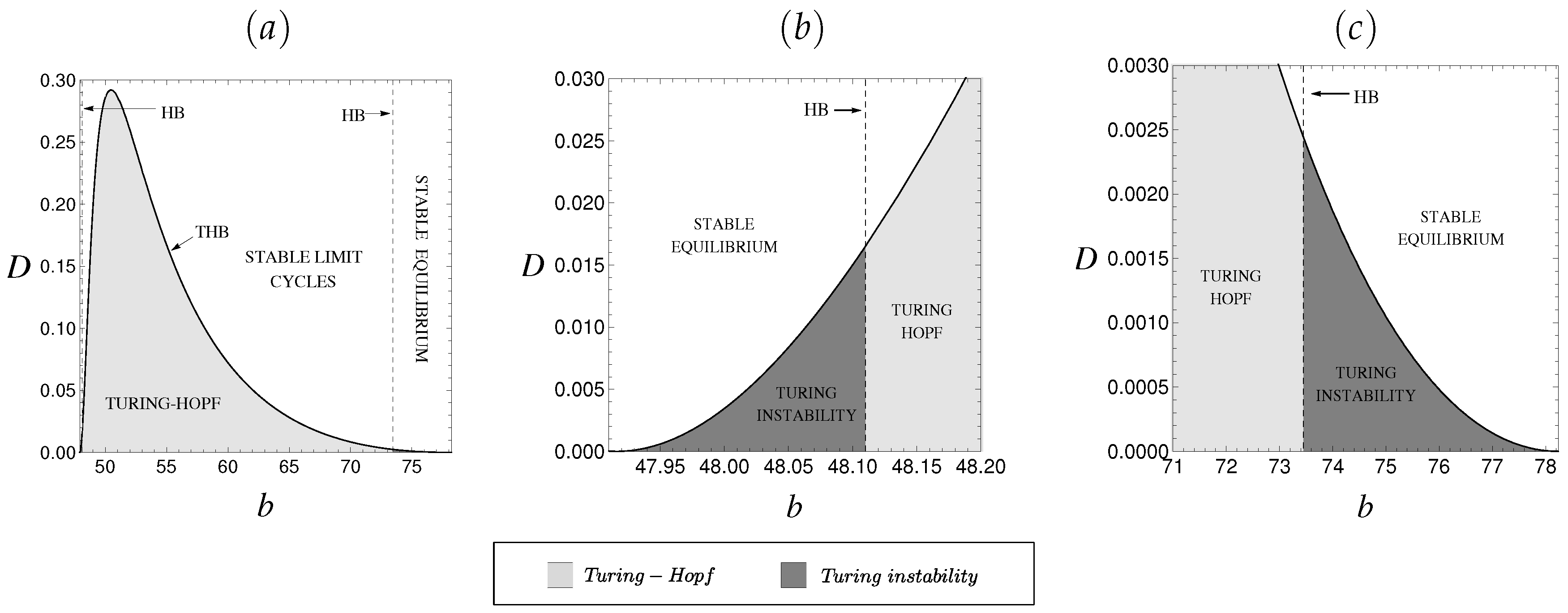
From our previous comments, Turing instability can only be possible when the equilibrium occurs in an increasing region of the n-nullcline. For parameters’ set I, this happens for b in the gray interval of Figure 2a. For b in the dark gray region, the equilibrium is stable and Turing instability condition (23) can be satisfied for some values of D. For parameters in light gray interval, the coexistence equilibrium is unstable and limit cycles are observed what suggests possible Turing-Hopf instabilities for suitable values of D.
Through this analysis we restricted our attention to the range of b for which diffusion driven instabilities are possible. We then, numerically verify the values of D for which condition (23) is satisfied. The only restriction for D is 0 < D < 1 since D 2 < D 1 . Figure 3 illustrates the region in the b , D parameters space where Turing and/or Turing-Hopf instabilities take place while Figure 4 indicates the types of pattern obtained for different combinations of the parameters b and D inside these regions.
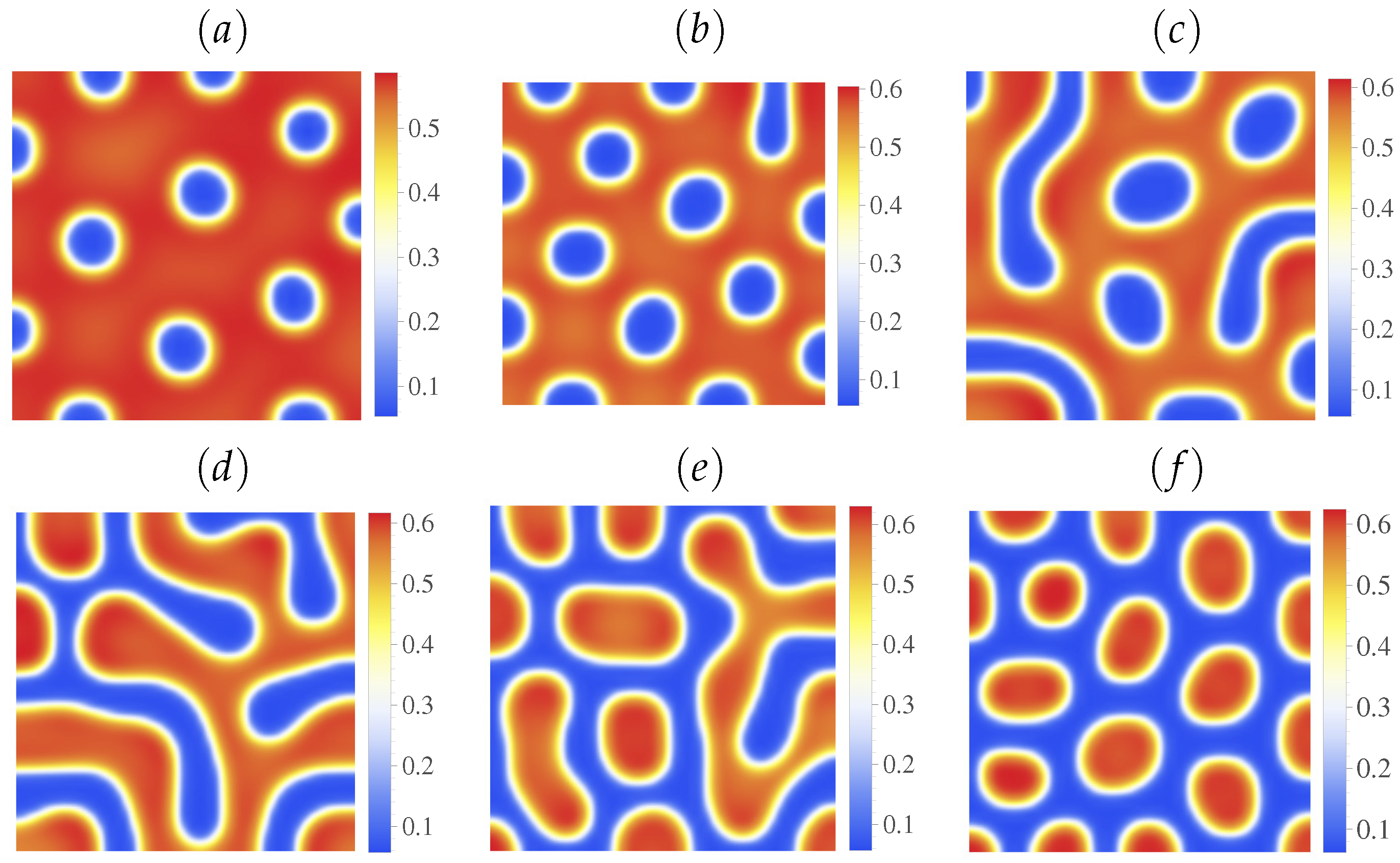
Examples of patterns obtained for parameters inside the Turing-Hopf region are illustrated in Figure 5. We can observe that increasing b and keeping D = 0.01 , the resulting pattern evolves from cold spots to hot spots after passing by a transition of stripes patterns. For grater values of D even though inside the Turing-Hopf region, the system evolves to a homogeneous population distribution. Since the equilibrium of the local dynamics is not stable for the parameters Set I with b inside this region; the system undergoes oscillations according to the corresponding limit cycle. Hence, the spatial dynamics exhibit time-oscillating homogeneous distributions.
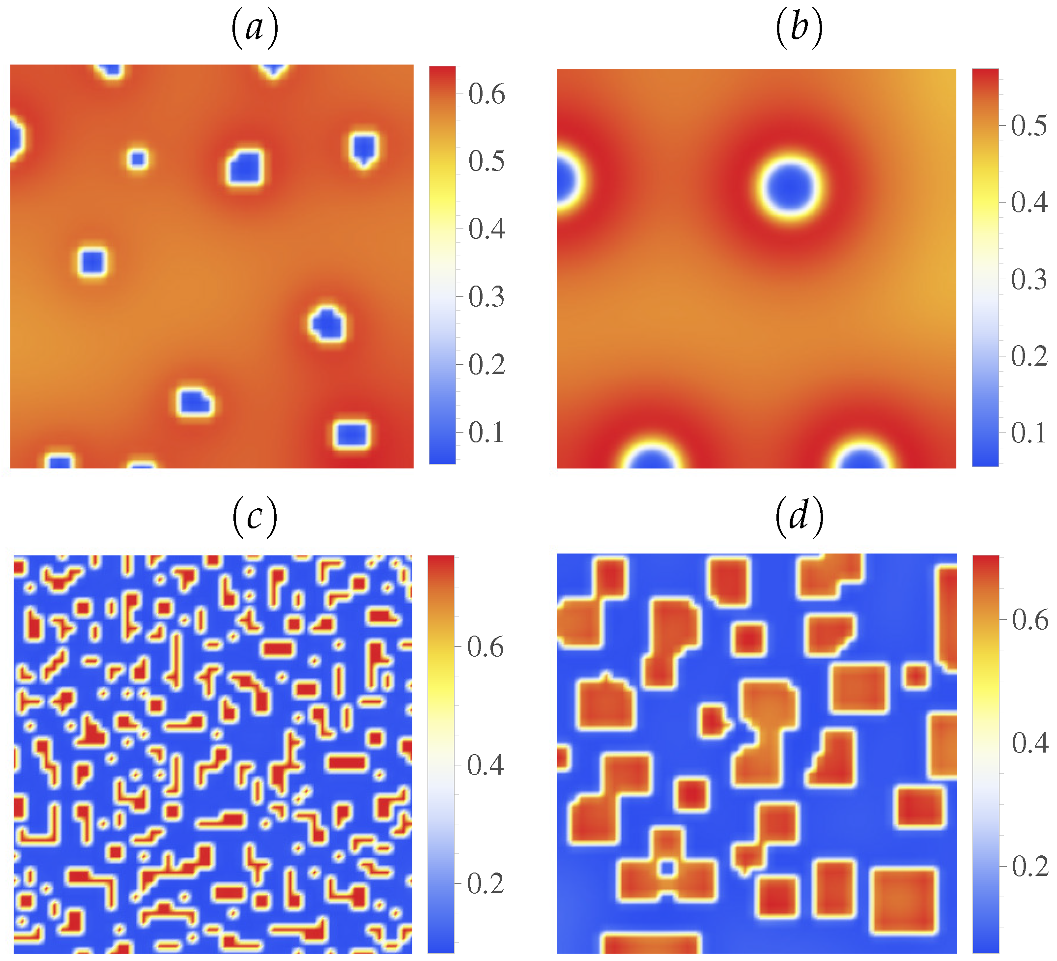
For parameters taken inside the Turing instability region of the parameters illustrated in Figure 4b we obtained cold spots as resulting patterns (see Figure 6a,b for examples). On the other hand, with parameters inside the Turing region illustrated in Figure 4c, spikes and hot spots were observed as, for example, those showed in Figure 6c,d, respectively.

5.2. Set II

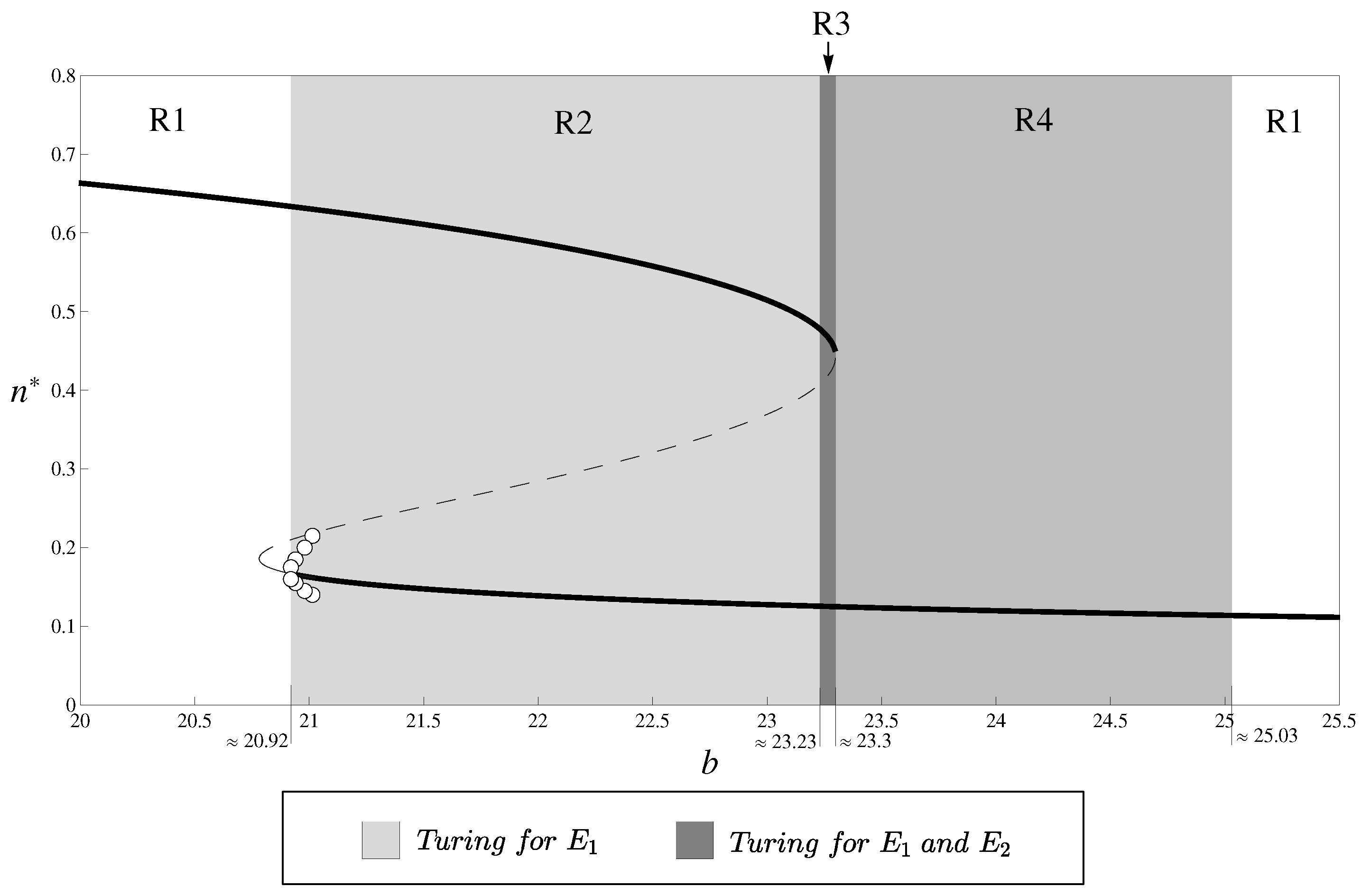
For parameters set II, the system exhibits bistability and unstable limit cycles as illustrated in Figure 7. It suggests that it would be possible, for the same parameter range, two different pattern regimes depending on whether the initial perturbation is made around one or another equilibrium. Furthermore, one can ask about the influence of one equilibrium on the other. We will refer to the equilibrium with small prey density as E 1 and to the equilibrium with high prey density as E 2 .
For b < 20.23 , E 2 is located where the n-nullcline is decreasing. Hence, condition (23) is not satisfied and Turing pattern is not possible for any perturbation of this equilibrium. For 20.92 < b < 25.03 approximately, which includes regions R 2 , R 3 and R 4 of Figure 7, the diffusive instability conditions (21)–(23) are satisfied for equilibrium E 1 . For b in the small interval R 3 Turing instability is possible for both equilibria.
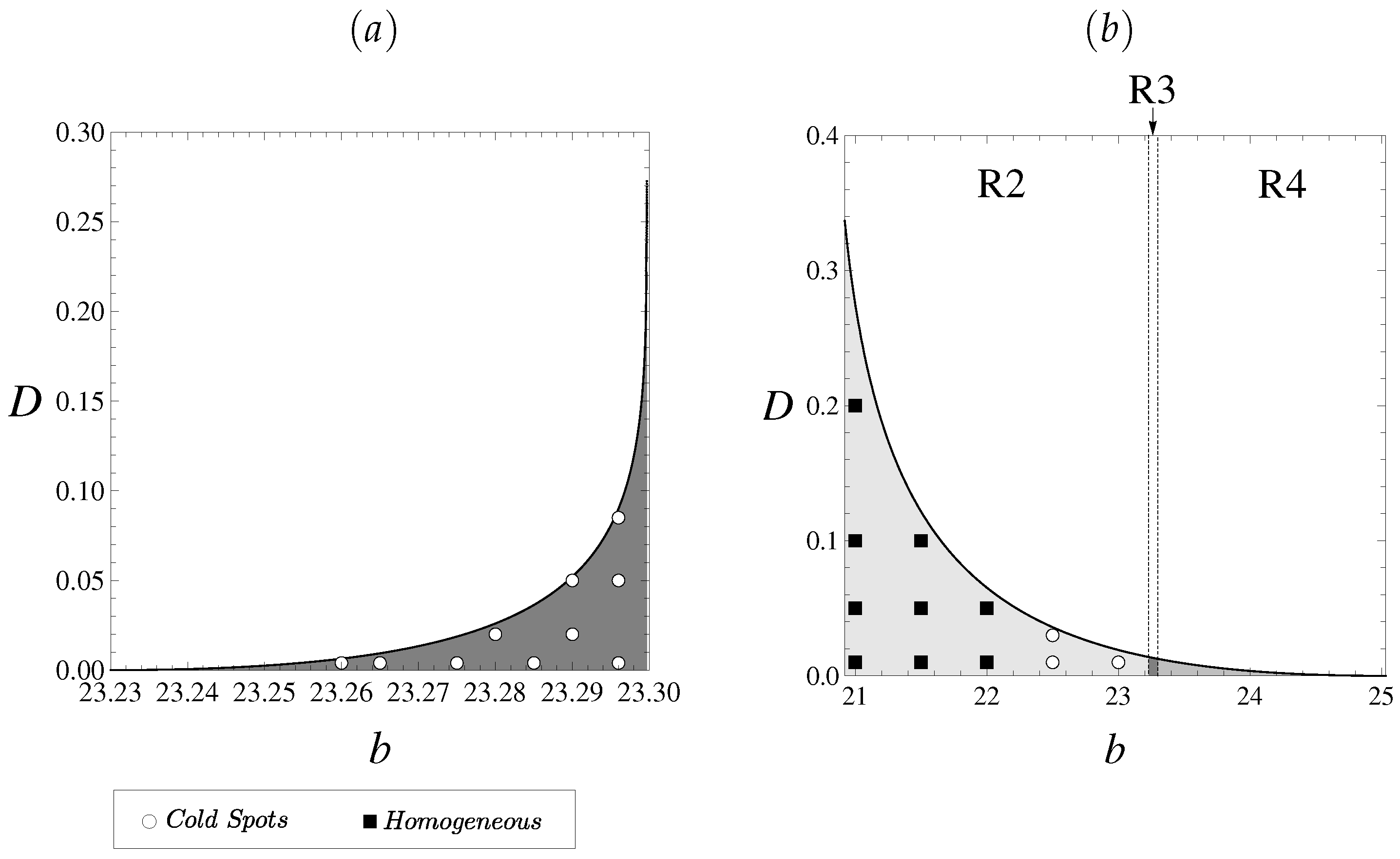
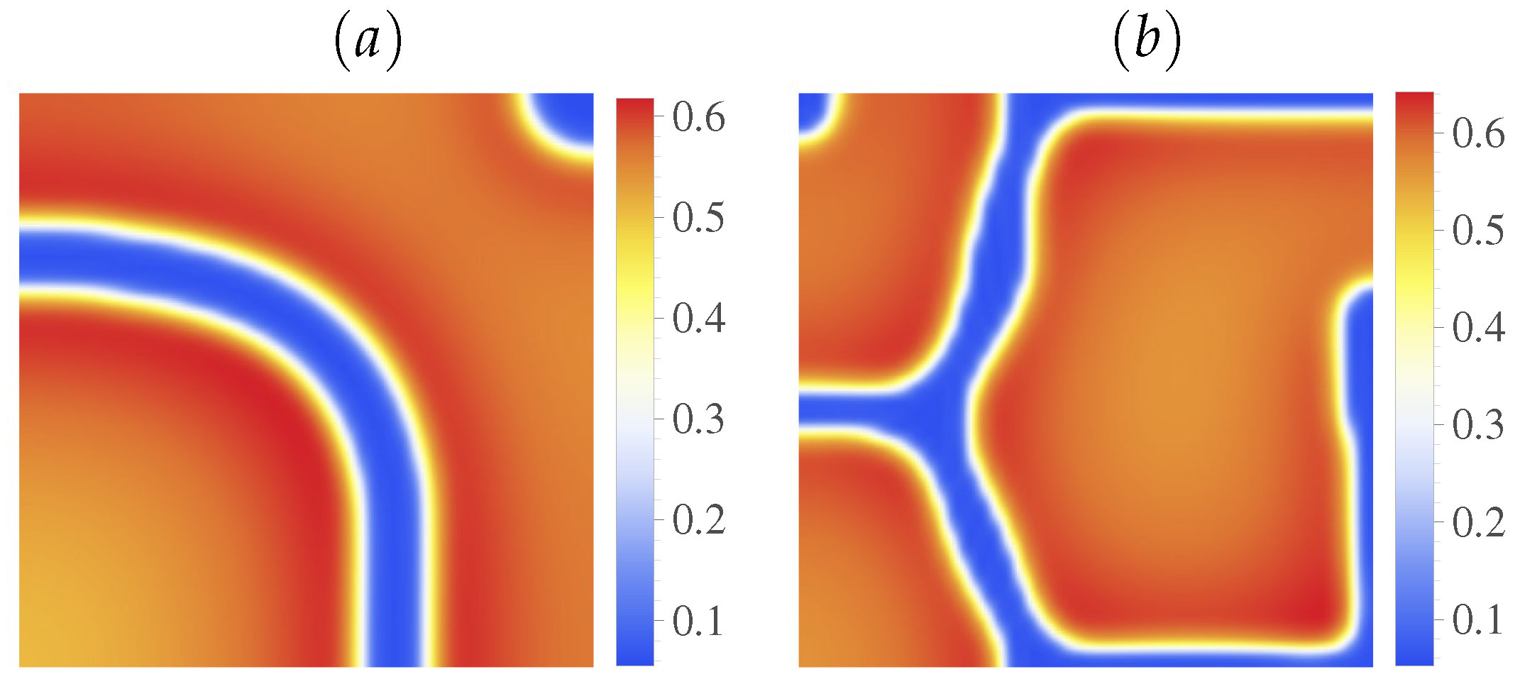
We then applied condition (23) for both equilibria in order to find the combinations of b and D for which Turing instability can happen. Figure 8a,b illustrate these regions for the equilibrium E 2 and E 1 , respectively. For b in R 3 and D taken in the dark gray region of Figure 8a, small perturbation of equilibrium E 2 , lead the species distributions to cold spots. For the equilibrium E 1 , on the other hand, we obtained different results. For very small values of D ( D < 0.005 approximately) regardless the value of b in the interval 20.92 < b < 25.03 which includes regions R 2 to R 4 , small heterogeneous initial perturbations lead to non-homogeneous patterns as those illustrated in Figure 9. On the other hand, as D increases, cold spots and heterogeneous stripes like patterns as illustrated in Figure 10 are obtained in regions R 2 and R 3 .
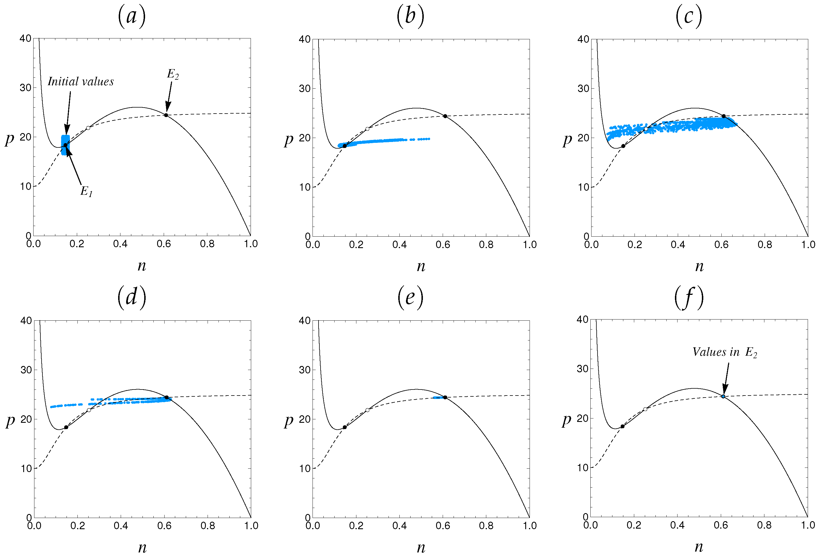
An interesting phenomenon is observed in region R 2 . For b close to region R 3 , initial perturbations of equilibrium E 1 lead to heterogeneous cold spots as those illustrated in Figure 5a. However, for small values of b in region R 2 (approximately 20.92 < b < 22 ) and D 0.005 initial perturbations around E 1 grow and the prey is lead to a homogeneous distribution at the equilibrium E 2 as represented in Figure 11. The blue points indicate the prey and predator densities in all the domain. For t = 0 (Figure 11a), all the points are around the equilibrium E 1 . Without diffusion, all the values would converge to E 1 . However, with diffusion, the solution in all the domain migrate during the transients (see Figure 11b–e) and finally tend to equilibrium E 2 (Figure 11f), even though the parameters belong to the Turing region. Nevertheless, there is no contradiction with Turing’s theory since it does not state that when diffusion is present, heterogeneous patterns will necessarily takes place. It says that the homogeneous distribution is unstable to small perturbations, what is the case here: perturbations around E 1 grow and the system is led to a uniform distribution at the equilibrium value E 2 . This phenomenon promotes a rupture of the effect of hysteresis observed in the local dynamics; in the spatially distributed model, the system state jumps from E 1 to E 2 due to perturbations caused by movement even though the initial distribution is inside the basin of attraction of E 1 . We also observe that the unstable limit-cycles observed for small values b in R 2 (see Figure 7) do not have any influence on the patterns obtained (for D < 0.005 ) and on the solution migration to E 2 (for greater values of D).

5.3. Set III

Parameters’ set III presents a much more complex local dynamics than the previous two cases. Differently from Set II, no bistability is observed. However, there is the coexistence of a stable equilibrium with a stable limit-cycle. We detected six intervals of b with different behaviour related to pattern formation which will be explained in what follows.
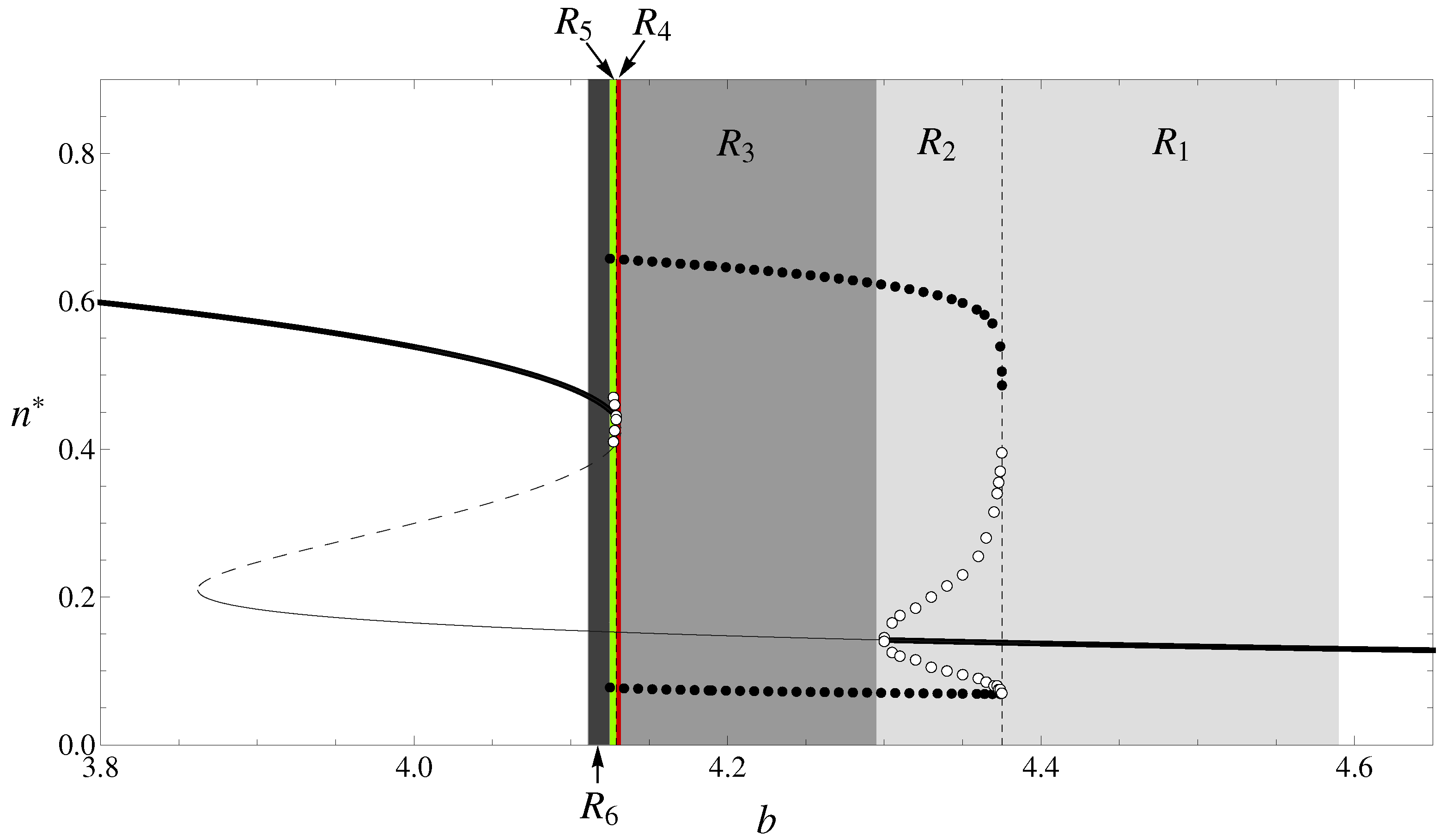
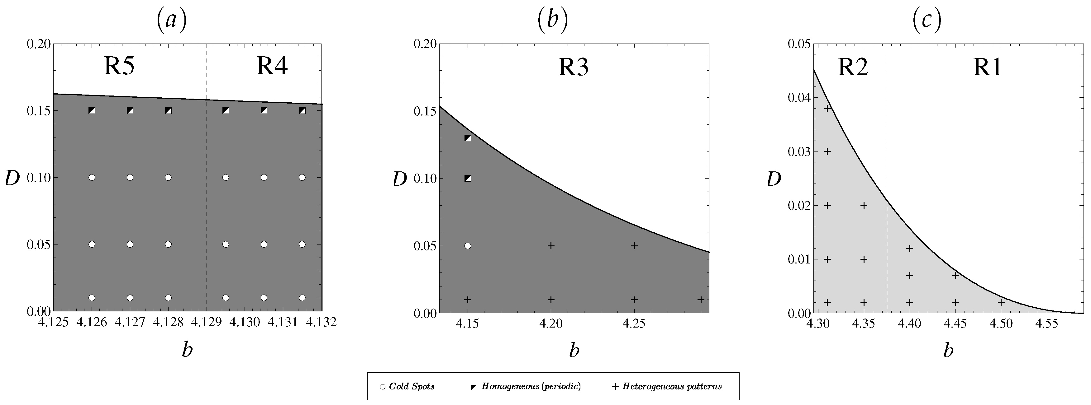
Figure 12 illustrates the bifurcation diagram for the prey with parameter b as controlling parameter. We will call E 1 the prey equilibrium with lower density and E 2 the higher prey equilibrium value. Figure 13 and Figure 14 show the combinations of parameters b and D for which diffusive instability is obtained, respectively, for equilibrium E 1 and E 2 in different intervals for b. The dots in these two figures indicate the combinations tested and the type of pattern obtained.
In the intervals corresponding to R 1 of Figure 12, E 1 is the only stable equilibrium. All the diffusive instability conditions are satisfied and hence, Turing patterns are possible for E 1 in R 1 . For D in gray region of Figure 13c, different heterogeneous patterns and stripes were obtained.
In R 2 of Figure 12, E 1 is still stable but now it is surrounded by two limit-cycles: one unstable and the other stable. Turing patterns are possible for E 1 in R 2 since all the conditions for diffusive instability can be satisfied for suitable combinations of b and D. The resulting patterns for D taken inside the corresponding gray region R 2 of Figure 13c are heterogeneous patterns. Since for b in R 2 there is an unstable limit-cycle surrounding E 1 , we initially perturbed this equilibrium up to 1 % of its value in each point.
For b in region R 3 , E 1 becomes unstable but the stable limit cycle is still surrounding it (see Figure 12). The condition (23) can still be satisfied what characterize region R 3 as a region where Turing-Hopf patterns are possible. For small values of D inside the gray region of Figure 13b, heterogeneous patterns and cold spots are obtained. However, with larger values of D, still inside the Turing region, the system is driven to a homogeneous periodic distribution which assumes the corresponding values of the stable limit cycle that surrounds E 1 .
Regions R 4 and R 5 are Turing-Hopf regions for E 1 since it is an unstable equilibrium surrounded by a stable limit-cycle. The combinations of b and D for which diffusive instability is observed can be seen in Figure 13a. Small perturbations of the homogeneous equilibrium distributions lead to heterogeneous as well as homogeneous periodic solutions for b and D in these regions. Cold spots patterns appear for low values of D in both regions R 4 and R 5 while homogeneous periodic solutions can be seen for larger values of D.
A saddle-node bifurcation takes place as b cross the border of region R 3 towards R 4 and the equilibrium E 2 , at high prey levels, appears. E 2 , which is also unstable for all values of b in R 4 , is surrounded by a stable limit-cycle. However, condition (23) holds for b and D in a certain range of values as illustrated in Figure 14c, which characterizes it as a Turing-Hopf region for equilibrium E 2 . We tested several combinations of parameters in this region and observed cold spots patterns for low values of D. For higher values of D, still inside the gray region, homogeneous periodic solutions are obtained. We can observe an unstable limit-cycle around E 2 ; with high values of D, the population values in all the domain jump outside this cycle and the system is lead to the stable outer cycle. It is worth noting that R 4 is also a Turing-Hopf region for equilibrium E 1 as mentioned above.
Moving b to region R 5 , equilibrium E 2 becomes stable. However, it is surrounded by an unstable limit-cycle and by the outer stable limit-cycle. All the conditions (21) to (23) can be satisfied for E 2 in this region. For b and D the region illustrated in Figure 14b, the Turing patterns obtained are cold spots.
Finally, for b in region R 6 , both limit-cycles disappear and E 2 is still stable. In R 6 the diffusive instability conditions can be satisfied only for E 2 if D is taken in the appropriate range illustrated in Figure 14a. Cold spots are the kind of distribution we obtained in this case.

6. Discussion

In this paper, we have analysed the effects of spatial distribution and species movement on the generalist predator-prey dynamics studied by Erbach et al. (2013) [27]. In particular, we have investigated the scenarios of pattern formation in the rich dynamics that the above mentioned authors proposed. Our main goal was to elucidate how is pattern formation influenced by limit-cycles and bistability present in the rich local dynamics. We then derived the conditions for Turing instability and developed numerical simulations for different sets of relevant parameters for the local kinetics. We found the regions in the parameter space b (related to the predation intensity) and D (the relation between prey and predator motility) for which Turing and Turing-Hopf patterns can be obtained, in most cases, for parameters far way from the bifurcation. By means of numerical simulations, we observed that hot spots, cold spots, stripes and a mixture of them can emerge depending on the predation intensity. With small values of b, predation on the focal prey is low and we observe isolated regions of lower prey (and predator) density; that is, cold spots are the typical patterns for low values of b. On the other hand, when predation is high (great values of b), the prey remains confined to limited regions of habitat in the so called hot spots patterns if predator movement rate is great compared to the prey. As consequence, the type of pattern can be associated with the effectiveness of the predator on controlling the focal prey. If hot spots are observed, prey density is around its low equilibrium level.

6.1. Spatiotemporal Chaos

In the Turing-Hopf instability domain, we obtained either stationary patterns (for small values of D, including hot/cold spots and stripes depending on b) or oscillating homogeneous distributions (for larger values of D). Spatiotemporal chaos, frequently observed in specialist [20,21] as well as generalist [25] predator-prey systems for parameters, close or inside, the Turing-Hopf instability regions, was not observed for any combinations of parameters, neither close the bifurcation nor into the region where chaotic behaviour would be expected. We also simulated Equation (2), for the parameters set III with b = 4.2 and D = 0.05 ; that is, inside the Turing-Hopf domain, from the initial perturbations n ( x , y , 0 ) = n * + 0.01 sin ( ε ( y 20 ) ) and p ( x , y , 0 ) = p * + 0.01 sin ( ε ( y 20 ) ) , for ε = 0.006 , ε = 0.025 and ε = 0.25 . In all these simulations the system also converged to either stationary heterogeneous patterns or homogeneous oscillating distributions. None of the initial perturbation tested, produced spatiotemporal chaos.
Contrary to [20,31] who found spatially irregular non-stationary patterns and spatiotemporal chaos for parameters in the vicinity of a Turing-Hopf bifurcation, Banerjee and Petrovskii [21] obtained heterogeneous stationary patterns for parameters close to this type of bifurcation. Spatiotemporal chaos, nonetheless, was obtained in [21] for parameters into the Turing-Hopf range. Furthermore, there are evidences that Turing instability is not necessary to trigger chaos; Banerjee and Petrovskii [21] showed that chaotic spatial patterns can appear in a specialist predator-prey system, outside the Turing domain, as a result of non-homogeneous perturbations in a region of parameters where limit-cycles are present in the local dynamics. We then tested the above mentioned parameters in set III with D = 1 (that is, outside the Turing domain) and again no irregular spatiotemporal pattern was observed. Chakraborty [25] have obtained chaotic spatiotemporal oscillations in a generalist predator-prey interaction, however in his model, predation occurs according to the Holling type II functional response. Our results, on the other hand, indicate that neither Turing-Hopf nor Hopf bifurcations can always be associated with spatiotemporal chaos in continuous reaction-diffusion predator-prey systems. A similar behaviour has already been found by Rodrigues and colleagues [32] in a discrete Coupled Map Lattice for predator-prey system, in which stationary patterns are observed even when the local dynamics is oscillatory. Although more investigation is needed, our findings suggest that the Holling type III function response such as we have used in the present work, may have a stabilizing effect on the spatiotemporal behaviour of the generalist predator-prey dynamics.

6.2. Bistability and Regime Shifts

The model studied here presents bistability that emerge from saddle-node bifurcations, which is the scenario for jumps and hysteresis to occur [33].
When the prey is an agricultural pest controlled by the generalist predator, the hysteresis effect observed in the local dynamics means that once the prey density falls from the high equilibrium density E 2 to the desired low equilibrium E 1 , as a result of increasing b, predation efforts can be relaxed to keep the control. That is, the pest density would only grow back to the high level E 2 if the predation decreases below the leftmost saddle-node bifurcation point, called now b c 1 (see Figure 7). Our results, nonetheless, show that spatial movement of the species (as it occurs with many species in real world plantations) may cause a shift back of the prey density to the upper levels if predation intensity is slightly relaxed below the level that causes the prey density decay, the rightmost saddle-node bifurcation point b c 2 . Close to this parameter value, the basin of attraction of the lower density equilibrium E 1 is considerable large (see Figure 7) so that, small perturbations caused by movement do not promote a shift back to high density E 2 . However, as the parameter b decreases from b c 2 , the basin of attraction of E 1 and consequently, its resilience, diminishes. Now, in the reaction-diffusion model, for values of b > b c 1 , perturbations due to movement can promote the shift back to high prey densities, in what we call an hysteresis break due to movement. In terms of pests control, our results suggest that in order to keep the prey at low densities, predation efforts should be kept as close as possible to b c 2 .
From a different perspective, if the prey is an endangered specie to be conserved, the regime shift and hysteresis described above may be undesirable since a regime shift can be hard to revert. From the species conservation point of view, it is important to detect regime shifts prior to its occurrence and there has been considerable effort of modelers to find hints that help identifying that the system is close to a regime shift and designing strategies of control to preventing catastrophes [28,34,35,36]. In the present study, we observed that for the upper prey equilibrium E 2 (see regions R 3 and R 6 in Figure 7 and Figure 12, respectively), pattern formation is only observed close to the catastrophic transition value. The typical patterns observed in this case are cold spots what suggests that when the prey species under predation of a generalist predator, starts being scarce in some geographical regions, it may be a signal that some dramatic change is approaching if predation pressure increases. Since the avoidance of regime shifts demands the development and implementation of strategies of control, the indication of a regime shift close to its occurrence may, unfortunately, represent another difficulty of impending it. Our results, thus suggest that monitoring ecological systems is essential for impeding regime shifts.
We hope that our results can, from one hand side, address part of the questions raised by Erbach and colleagues and, on the other side, instigate researchers interested in population dynamics to further investigate generalist predator-prey interactions.

Author Contributions

The authors have contributed equally to this work. All authors have read and agreed to the published version of the manuscript.

Funding

VWR was funded by Coordenação de Aperfeiçoamento de Pessoal de Nível Superior.

Conflicts of Interest

The authors declare no conflict of interest.

References

  1. Gibert, J.P.; Yeakel, J.D. Laplacian matrices and Turing bifurcations: Revisiting Levin 1974 and the consequences of spatial structure and movement for ecological dynamics. Theor. Ecol. 2019, 12, 265–281. [Google Scholar] [CrossRef] [Green Version]
  2. Nicholson, A.J.; Bailey, V.A. The balance of animal population. Part I. Proc. Zool. Soc. Lond. 1935, 3, 551–598. [Google Scholar] [CrossRef]
  3. Comins, H.N.; Hassell, M.P.; May, R.M. The spatial dynamics of host-parasitoid systems. J. Anim. Ecol. 1992, 61, 735–748. [Google Scholar] [CrossRef]
  4. Hassell, M.P.; Comins, H.N.; May, R.M. Spatial structure and chaos in insect population dynamics. Nature 1991, 353, 255–258. [Google Scholar] [CrossRef]
  5. Cantrell, R.S.; Cosner, C. Spatial Ecology via Reaction-Diffusion Equations; Wiley: London, UK, 2003. [Google Scholar]
  6. Edelstein-Keshet, L. Mathematical Models in Biology; Random House: New York, NY, USA, 1988. [Google Scholar]
  7. Holmes, E.E.; Lewis, M.A.; Banks, J.E.; Veit, R.R. Partial differential equations in ecology: Spatial interactions and populations dynamics. Ecology 1994, 75, 17–29. [Google Scholar] [CrossRef]
  8. Okubo, A.O.; Levin, S.A. Diffusion and Ecological Problems. Modern Perspectives; Springer: New York, NY, USA, 2001. [Google Scholar]
  9. Lewis, M.A.; Kareiva, P. Allee dynamics and the spread of invading organisms. Theor. Pop. Biol. 1993, 43, 141–158. [Google Scholar] [CrossRef]
  10. Owen, M.; Lewis, M.A. How predation can stop, slow or reverse a prey invasion. Bull. Math. Biol. 2001, 63, 655–689. [Google Scholar] [CrossRef] [Green Version]
  11. Sherratt, J.A.; Lewis, M.A.; Fowler, A.C. Ecological chaos in invasion. Proc. Natl. Acad. Sci. USA 1995, 92, 2524–2528. [Google Scholar] [CrossRef] [Green Version]
  12. Shigesada, N.; Kawasaki, K. Biological Invasions: Theory and Practice; Oxford University Press: Oxford, UK, 1997. [Google Scholar]
  13. Kierstead, H.; Slobodkin, L.B. The size of water masses containing plankton blooms. J. Mar. Res. 1953, 12, 141–147. [Google Scholar]
  14. Malchow, H.; Petrovskii, S.V.; Venturino, E. Spatiotemporal Patterns in Ecology and Ecoepidemiology: Theory, Models, and Simulations; Champman & and Hall: London, UK, 2008. [Google Scholar]
  15. Murray, J.D. Mathematical Biology II: Spatial Models and Biomedical Applications, 3rd ed.; Springer: Berlin, Germany, 2003. [Google Scholar]
  16. Segel, L.A.; Jackson, J.L. Dissipative structure: an explanation and an ecological example. J. Theor. Biol. 1972, 37, 545–559. [Google Scholar] [CrossRef]
  17. Turing, A.M. The chemical basis of morphogenesis. Phil. Trans. R. Soc. Lond. B 1952, 237, 37–72. [Google Scholar]
  18. Gierer, A.; Meinhardt, H. A theory for biological pattern formation. Kybernetik 1972, 12, 30–39. [Google Scholar] [CrossRef] [PubMed] [Green Version]
  19. Meinhardt, H. Models of Biological Pattern Formation; Academic Press: London, UK, 1982. [Google Scholar]
  20. Baurmann, M.; Gross, T.; Feudel, U. Instabilities in spatially extended predator-prey systems: Spatio-temporal patterns in the neighborhood of Turing-Hopf bifurcations. J. Theor. Biol. 2007, 245, 220–229. [Google Scholar] [CrossRef] [PubMed] [Green Version]
  21. Banerjee, M.; Petrovskii, S. Self-organized spatial patterns and chaos in a ratio-dependent predator-prey system. Theor. Ecol. 2011, 4, 37–53. [Google Scholar] [CrossRef]
  22. Morozov, A.; Petrovskii, S. Excitable population dynamics, biological control failure, and spatiotemporal pattern formation in a model ecosystem. Bull. Math. Biol. 2009, 71, 863–887. [Google Scholar] [CrossRef]
  23. Kumari, N. Pattern formation in spatially extended tritrophic food chain model systems: Generalist versus specialist top predator. ISRN Biomath. 2013, 2013, 198185. [Google Scholar] [CrossRef] [Green Version]
  24. Magal, C.; Cosner, C.G.; Ruan, S.; Casas, J. Control of invasive hosts by generalist parasitoids. Math. Med. Biol. 2008, 25, 1–20. [Google Scholar] [CrossRef] [Green Version]
  25. Chakraborty, S. The influence of generalist predators in spatially extended predator-prey systems. Ecol. Complex. 2015, 23, 50–60. [Google Scholar] [CrossRef] [Green Version]
  26. Holling, C.S. Some characteristics of simple types of predation and parasitism. Can. Entomol. 1959, 91, 385–398. [Google Scholar] [CrossRef]
  27. Erbach, A.; Lutscher, F.; Seo, G. Bistability and limit cycles in generalist predator-prey dynamics. Ecol. Complex. 2013, 14, 48–55. [Google Scholar] [CrossRef]
  28. Biggs, R.; Carpenter, S.R.; Brock, W.A. Turning back from the brink: Detecting an impeding regime shift in time to avert it. Proc. Natl. Acad. Sci. USA 2009, 106, 826–831. [Google Scholar] [CrossRef] [PubMed] [Green Version]
  29. Segel, L.A. Modeling Dynamic Phenomena in Molecular and Cellular Biology; Cambridge University Press: Cambridge, UK, 1984. [Google Scholar]
  30. Jones, D.S.; Sleeman, B.D. Differential Equations and Mathematical Biology; Chapman & Hall/CRC: London, UK, 2003. [Google Scholar]
  31. Meixner, M.; De Wit, A.; Bose, S.; Scholl, E. Generic spatiotemporal dynamics near codimension-two Turing-Hopf bifurcations. Phys. Rev. E 1997, 55, 6690–6697. [Google Scholar] [CrossRef]
  32. Rodrigues, L.A.D.; Mistro, D.C.; Petrovskii, S. Pattern Formation, Long-Term Transients, and the Turing–Hopf Bifurcation in a Space- and Time-Discrete Predator–Prey System. Bull. Math. Biol. 2011, 73, 1812–1840. [Google Scholar] [CrossRef] [PubMed]
  33. Strogatz, S.H. Nonlinear Dynamics and Chaos. With Applications to Physics, Biology, Chemistry, and Engineering, 2nd ed.; Westview Press: Philadelphia, PA, USA, 2015. [Google Scholar]
  34. Kéfi, S.; Maarten, B.E.; de Ruiter, P.C.; Rietkerk, M. Bistability and regular patterns in arid systems. Theor. Ecol. 2010, 3, 257–269. [Google Scholar] [CrossRef] [Green Version]
  35. Rietkerk, M.; Dekker, S.C.; de Ruiter, P.C.; van de Koppel, J. Self-Organized Patchiness and Catastrophic Shifts in Ecosystems. Science 2004, 305, 1926–1929. [Google Scholar] [CrossRef] [Green Version]
  36. Scheffer, M.; Carpenter, S.; Foley, J.A.; Walker, B. Catastrophic shifts in ecosystems. Nature 2001, 413, 591–596. [Google Scholar] [CrossRef] [PubMed]
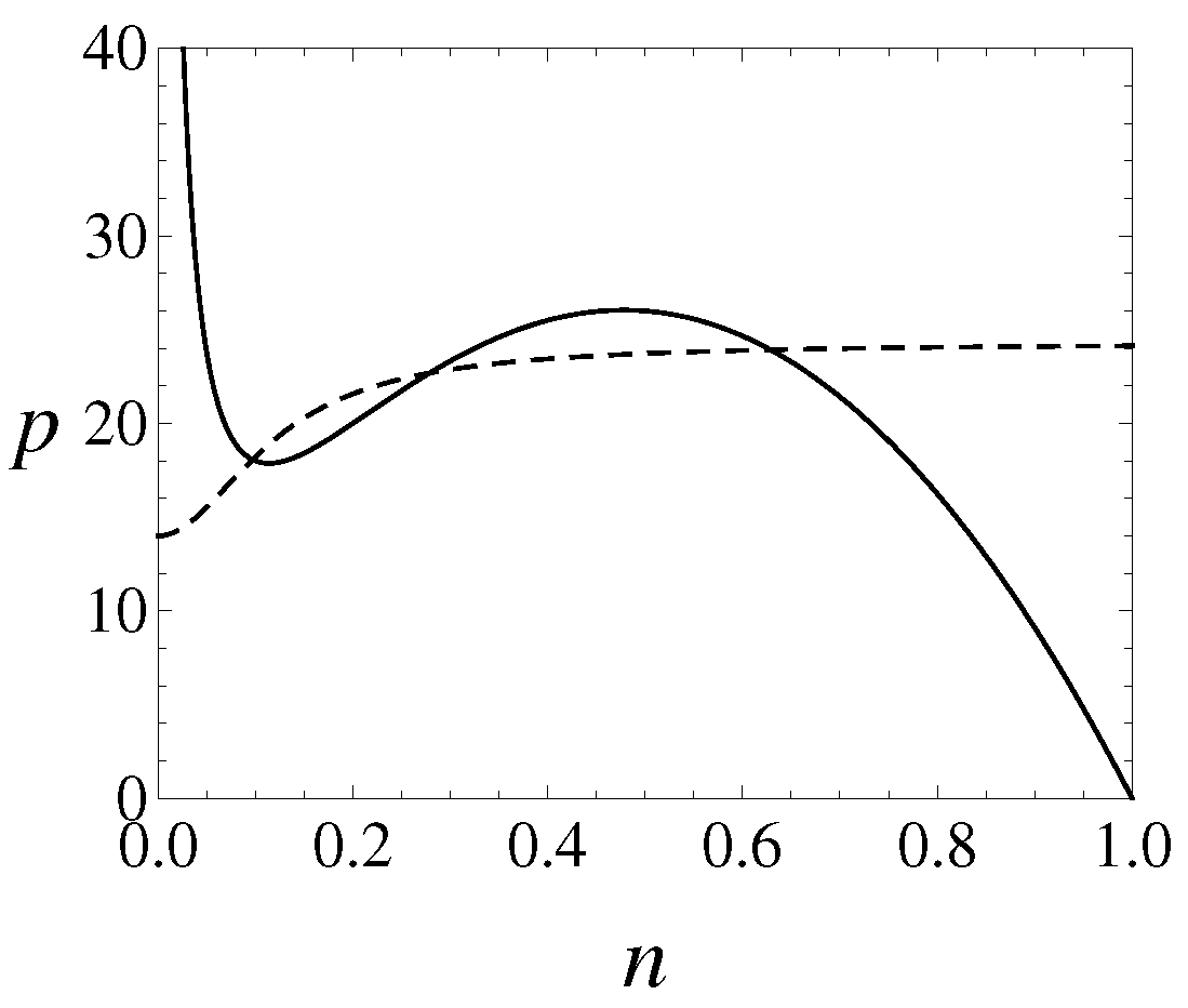
Figure 1. Possible shape of the local model nullclines. The continuous and dashed curves represent the graphic of f and g, respectively. f has two local extreme ( a > 27 ) and g has an upper limit ( b < a e ).
Mathematics 08 00020 g001
Figure 2. (a) Bifurcation diagram for prey species with b as the controlling parameter. The continuous (dashed) line indicates the stable (unstable) steady state. Black dots are the maximum and minimum prey density in the stable limite cycle. (b) Phase plane for different values of b. The continuous curve corresponds to one nullcline for prey while the dashed curves represent p-nullclines for different values of b. Black (white) dots represent the stable (unstable) coexistence equilibrium. In both images, other parameters are given by Set I.
Mathematics 08 00020 g002
Figure 3. (a) Stability diagram in the b × D parameters space. (b,c) represent a zoom for a better visualization of the Turing instability region. HB stands for Hopf Bifurcation and THB indicates Turing Hopf Bifurcation.
Mathematics 08 00020 g003
Figure 4. Pattern types obtained for different combinations of b and D inside the Turing-Hopf region (a) and inside Turing regions, illustrated in a zoom in (b,c).
Mathematics 08 00020 g004
Figure 5. Prey spatial distribution in Turing-Hopf region for D = 0.01 and different values of b: (a) b = 50 , (b) b = 52.5 , (c) b = 55 , (d) b = 57.5 , (e) b = 60 and (f) b = 65 .
Mathematics 08 00020 g005
Figure 6. Example of patterns obtained in the two different Turign regions: (a) b = 48.07 and D = 0.002 ; (b) b = 48.07 and D = 0.01 ; (c) b = 74 and D = 0.0002 and (d) b = 74 and D = 0.0015 .
Mathematics 08 00020 g006
Figure 7. Bifurcation diagram for the prey equilibrium with regard to b with the remainder parameters fixed as in Set II. The black bold parts of the curve indicate stable equilibria while thin and dashed curves stand for unstable equilibria. The white dots represent unstable limit-cycles. In the white regions labeled R 1 no Turing pattern is possible. Turing instabilities are feasible in the light and dark gray regions as explained in the text.
Mathematics 08 00020 g007
Figure 8. Regions in the b D parameters space where all the diffusive instability conditions are satisfied for (a) E 2 and (b) E 1 .
Mathematics 08 00020 g008
Figure 9. Examples of Turing patterns obtained for equilibrium E 1 in different regions of the parameters b with very small values for D. Region R 2 : (a) b = 21.5 and D = 0.001 and, Region R 3 : (b) b = 23.24 and D = 0.001 .
Mathematics 08 00020 g009
Figure 10. Examples of Turing patterns obtained for equilibrium E 1 in different regions of the parameters b with greater values for D. Region R 3 : (a) b = 23.27 and D = 0.012 and, Region R 4 : (b) b = 23.5 and D = 0.008 .
Mathematics 08 00020 g010
Figure 11. n and p nullclines along with the values of prey and predator densities in the whole domain (indicated in blue), for b = 21.5 and D = 0.05 , at time: (a) t = 0 , (b) t = 60 , (c) t = 100 , (d) t = 120 , (e) t = 140 and (f) t = 200 .
Mathematics 08 00020 g011
Figure 12. Bifurcation diagram for the prey equilibrium with respect to b.
Mathematics 08 00020 g012
Figure 13. Regions in the b D parameters’ space where Turing or Turing-Hopf instabilities are obtained for equilibrium E 1 , illustrated in (ac) for better visualization. Dots indicate the combinations of parameters used for tests.
Mathematics 08 00020 g013
Figure 14. Regions in the b D parameters’ space where Turing or Turing-Hopf instabilities are obtained for equilibrium E 2 , illustrated in (ac) for better visualization. Dots indicate the spatial pattern obtained for the corresponding combination of parameters.
Mathematics 08 00020 g014