Pareto Explorer for Finding the Knee for Many Objective Optimization Problems

Abstract

Optimization problems where several objectives have to be considered concurrently arise in many applications. Since decision-making processes are getting more and more complex, there is a recent trend to consider more and more objectives in such problems, known as many objective optimization problems (MaOPs). For such problems, it is not possible any more to compute finite size approximations that suitably represent the entire solution set. If no users preferences are at hand, so-called knee points are promising candidates since they represent at least locally the best trade-off solutions among the considered objective values. In this paper, we extend the global/local exploration tool Pareto Explorer (PE) for the detection of such solutions. More precisely, starting from an initial solution, the goal of the modified PE is to compute a path of evenly spread solutions from this point along the Pareto front leading to a knee of the MaOP. The knee solution, as well as all other points from this path, are of potential interest for the underlying decision-making process. The benefit of the approach is demonstrated in several examples.

1. Introduction

In many applications, we are faced with several conflicting and incommensurable objectives that have to be optimized concurrently (e.g., Reference [1,2,3,4,5]). As a general example, for the design of a certain product, two important objectives are, in most cases, the cost of the product (to be minimized) and its quality (to be maximized), among other possible goals. Problems of this kind are termed multi-objective optimization problems (MOPs) in literature. One important characteristic of MOPs is that there is typically not one optimal solution to be expected (as for “classical” scalar optimization problems (SOPs)) but rather an entire set of solutions. More precisely, for continuous MOPs with k objectives, one can expect that the solution set (Pareto set) and its image (Pareto front) form at least locally objects of dimension $k-1$. Since there is a certain trend that decision-making processes are getting more complex, it comes as no surprise that also more and more objectives are being considered within such problems. Such problems are also termed many objective optimization problems (MaOPs). Though MOPs and MaOPs are identical mathematically, the above described “curse of dimensionality” calls for different numerical procedures for their treatment: while it is, in many cases, possible to compute suitable finite-size approximations of the entire Pareto sets/fronts of MOPs (e.g., Reference [1,6,7,8,9,10,11,12,13,14,15]), this becomes more challenging and even intractable with increasing number of objectives. There exist some evolutionary approaches that aim to compute finite size approximations of the entire solution sets for MaOPs. In Reference [16], a multi-objective evolutionary algorithm (MOEA) is presented that handles large population sizes (populations with up to 10,000 individuals). In Reference [17,18,19], dimension reduction techniques are proposed that aim to detect objectives that are not in conflict with each other. Finally, in Reference [20,21], large-scale MaOPs are addressed. All of these methods run into trouble for larger number of objectives due to the dimensionality issue.

An alternative is to restrict the search to one or few selected points or areas around the Pareto set/front. One possibility is to utilize users preferences, if such information is at hand. There already exist many scalarization methods (i.e., methods that transform the original MOP into a suitable SOP) that can incorporate such information directly, including the weighted sum method [22], the $ϵ$-constraint method [23], and the weighted Tchebycheff method [24], as well as reference point methods [25,26,27]. We refer to Reference [28,29] for more detailed discussion. The solutions of all of these methods depend next to several design parameters (which may reflect the users preferences) also on the shape of the Pareto front, which is apparently not known. Hence, it is rather unclear if these solutions are indeed the “ideal” solutions according to the given problem. The Pareto Explorer (PE [30]) is a global/local exploration tool for the numerical treatment of MaOPs: in a first step, one (or several) optimal solutions are computed and presented to the decision-maker. These could be the results of any of the above mentioned scalarization methods, or any other (preferably global) multi-objective solver. In a second step, the Pareto landscape is explored locally around the given solution according to the preferences of the decision-maker and the given solution. These preferences can be articulated in decision variable, objective, and weight space. Step 2 can hence be seen as a “fine tuning” of the solution that is computed in the first step.

In case no users preferences are at hand, knee points are potentially interesting candidates since they represent (at least locally) the best trade-off solutions among all the objectives involved in the problem [31,32,33,34,35,36,37,38,39,40]. For this, consider the hypothetical (and extreme) example that is depicted in Figure 1. Shown are the Pareto front of a bi-objective problem (assuming that both objectives have to be minimized), the convex hull of individual minima (CHIM) for this problem (which we will define in detail in the next section), and the images of two hypothetical points x and $\kappa$ (denote by $F\left(x\right)$ and $F\left(\kappa \right)$). We first consider the solution x. This solution might not be preferred by some decision-makers since there exist solutions those images are “left up” the Pareto front for which large gains with respect to $f_1$ may be obtained with only very small sacrifices according to $f_2$. Such extreme trade-offs cannot be obtained for $\kappa$, which is indeed the knee solution as defined by Das [41], which we will use in this work. While, so far, several methods exist for the computation of knees, they exclusively compute such solutions. Additionally, it would be interesting to locally explore the Pareto landscape around both the knee and the initial solution $x_0$, since decision-makers tend to compare the new candidates with $x_0$. If, for instance $x_0$ is placed in a high-quality niche for the above mentioned bi-objective design problem for a certain product, the resulting knee solution $\kappa$ may represent an unacceptable decrease of quality compared to $x_0$ even if this comes with a significant reduction of the cost.

In this paper, we will adjust the Pareto Explorer to find such knee solutions. More precisely, we will adapt the 2nd step of the algorithm so that it generates a sequence of (ideally uniformly distributed) solutions along the Pareto set/front leading to a local knee solution of a given MaOP. To this end, we will first (slightly) modify the definition of the knee. Originally, the knee solution has been proposed for problems with only a few objectives where the knee solution is typically in the “center” of the Pareto front. However, this changes when considering problems with more objectives and/or if the problem is degenerated (i.e., when the dimension of the Pareto set/front is less than $k-1$). The probability for the latter increases with the number of the considered objectives. As an example, consider the MaOP related to laundry design reported in Reference [30]: 13 out of the 14 considered objectives dealt with the ability of the laundry system to remove certain substances during the washing (namely wool greasy type A, wool grease type B, red wine, sebum type A, sebum type B, curry, motor oil, petroleum, blood, egg, starch, vegetable fat, and cocoa). It is even for the experts hard to decide (if not impossible) to know if all objectives are in conflict with each other, or if at least two of them share exactly the same characteristics. In the next step, we will adapt the Pareto Explorer to the context of knee finding using the modified definition of Das. We present the usefulness of the approach together with a comparison to the original method of Das (which we will call the NBI method) as far as it is possible. Results indicate that the PE approach is beneficial over the NBI method for higher-dimensional problems, and, as anticipated, for degenerated problems. However, we stress that the PE algorithm is designed to compute a path of equally distributed solutions along the Pareto front from an initial solution toward the knee solution (since all of these solutions are of potential interest for the decision-maker), which differs from the sole detection of the knee.

2. Background

In this section, we briefly state the main concepts and notations that will be used for the understanding of this work.

We will consider here continuous multi-objective optimization problems (MOPs) that can be defined mathematically as

$$\begin{array}{cc}\underset{x\in {\mathbb{R}}^n}{min}& F\left(x\right),\hfill \\ \mathrm{s}.\mathrm{t}.& g\left(x\right)\le 0\hfill \\ & h\left(x\right)=0,\hfill \end{array}$$

(1)

where $F:{\mathbb{R}}^n\to {\mathbb{R}}^k$ is the map of the k individual objectives $f_i:{\mathbb{R}}^n\to \mathbb{R}$. We assume that all objectives are sufficiently smooth. The domain of the functions is defined by

$$D:=\{x\in {\mathbb{R}}^n:g\left(x\right)\le 0andh\left(x\right)=0\}.$$

(2)

Optimality of a MOP is usually defined using the concept of dominance. Let $v,w\in {\mathbb{R}}^k$. Then, v is less than w (in short: $v{<}_{p}w$) if $v_i<w_i$ for all $i\in \{1,\dots ,k\}$ (analogously ${\le }_p$). $y\in D$ is dominated) by $x\in D$ ($x\prec y$) with respect to (1) if $F\left(x\right){\le }_{p}F\left(y\right)$ and $F\left(x\right)\ne F\left(y\right)$. A point $x\in D$ is called (Pareto) optimal or a Pareto point of (1) if there exists no $y\in D$ that dominates x. The set of all Pareto optimal solutions is called the Pareto set, i.e.,

$$\begin{array}{cc}\hfill P_D:=& \{x\in D:x\text{is a Pareto point of}(1\left)\right\}\hfill \\ \hfill =& \{x\in D:\nexists y\in D:y\prec x\}.\hfill \end{array}$$

(3)

The image $F\left(P_D\right)$ of $P_D$ is called the Pareto front. Typically, both Pareto set and front of a given multi-objective problem form at least locally a set of dimension $k-1$ [42]. Due to this “curse of dimensionality”, problems with more than, say, $k=4$ objectives are also called many objective optimization problems (MaOPs) in literature.

The first-order condition of optimality for differentiable MOP is given by the KKT equations, named after the work of Karush [43] and Kuhn and Tucker [44].

Theorem 1.

Suppose that$x^{*}$is a local solution of (1). Then, there exist Lagrange multipliers$\alpha \in {\mathbb{R}}^k$,$\lambda \in {\mathbb{R}}^p$and$\gamma \in {\mathbb{R}}^m$such that the following conditions are satisfied

$$\begin{array}{cc}\hfill J^T\alpha +\sum _{i=1}^p{\lambda }_i\nabla h_i\left(x^{*}\right)+\sum _{i=1}^m{\gamma }_i{g}_i\left(x^{*}\right)=0& \end{array}$$

(4)

$$\begin{array}{cc}\hfill h_i\left(x^{*}\right)=0,& i=1\dots p,\end{array}$$

(5)

$$\begin{array}{cc}\hfill g_i\left(x^{*}\right)\le 0,& i=1\dots m,\end{array}$$

(6)

$$\begin{array}{cc}\hfill {\alpha }_i\ge 0,& i=1\dots k,\end{array}$$

(7)

$$\begin{array}{cc}\hfill \sum _{i=1}^k{\alpha }_i=1,& \end{array}$$

(8)

$$\begin{array}{cc}\hfill {\gamma }_i\ge 0,& i=1\dots m,\end{array}$$

(9)

$$\begin{array}{cc}\hfill {\gamma }_i{g}_i\left(x^{*}\right)=0,& i=1\dots m,\end{array}$$

(10)

where $J=J\left(x\right)$ denotes the Jacobian of F at x,

$$J\left(x\right)=\left(\begin{array}{c}\nabla f_1{\left(x\right)}^T\\ ⋮\\ \nabla f_k{\left(x\right)}^T\end{array}\right)\in {\mathbb{R}}^{k\times n}.$$

(11)

One important aspect that we will need later on is that given a KKT point $x^{*}$, its associated weight vector ${\alpha }^{*}$, where ${\alpha }_i^{*}>0$, $i=1,\dots ,k$, is normal to the linearized Pareto front at $F\left(x^{*}\right)$ [42].

Das defined in Reference [41] the “knee” solution of a given MOP (or MaOP) as the solution to the following scalar optimization problem:

$$\begin{array}{ccc}& \hfill \underset{(x,t,\beta )}{max}& t\\ \mathrm{s}.\mathrm{t}.\\ & \hfill \Phi \beta +t\widehat{n}& =& F\left(x\right)-F^{*}\hfill \\ & \hfill e^T\beta & =& 1\hfill \\ & \hfill h\left(x\right)& =& 0\hfill \\ & \hfill g\left(x\right)& \le & 0\hfill \\ & \hfill {\beta }_i& \ge & 0,i=1,2,\cdots ,k.\hfill \end{array}$$

(12)

Hereby, $x\in {\mathbb{R}}^n$, $t\in \mathbb{R}$, $\beta \in {\mathbb{R}}^k$, $e={(1,\dots ,1)}^T\in {\mathbb{R}}^k$, and $F^{*}={(f_1^{*},\dots ,f_k^{*})}^T$ is the utopian vector that consists of the objective values $f_i^{*}=f_i\left(x_i^{*}\right)$ of the individual global minima $x_i^{*}\in D$. $\Phi$ is the $k\times k$ matrix in which i-th column vector is given by $F_i^{*}-F^{*}$, where $F_i^{*}=F\left(x_i^{*}\right)$. Finally, $\widehat{n}$ denotes the vector that is orthogonal to the hyperplane that contains the CHIM and that points toward the origin. If $(\overline{x},\overline{t},\overline{\beta })$ is a solution to (12), we call $\overline{x}$ a knee of MOP (1). For the bi-objective problem depicted in Figure 1, the knee solution is provided by $\kappa$.

The Pareto Explorer (PE), which we will use in this work, is a global/local exploration tool for the decision-making support in MaOPs. The PE consists of two steps as follows:

Step 1

Compute one (or several) optimal solution $x_0$ of the MaOP.

Step 2

Explore the Pareto landscape around $x_0$ via performing movements into user-specified directions.

Step 1 can be performed via in principle any (preferably global) multi-objective solver, such as any of the above mentioned scalarization methods or a MOEA [45,46,47,48], that will return an entire set of solutions. For the latter, part of Step 1 will be then that the decision-maker selects one element $x_0$ out of this set (while the approach can of course be repeated with any other the other solutions). The following Step 2 is the “fine tuning” of $x_0$, respectively, its image $F\left(x_0\right)$. For this, either an unbiased overview of the possible alternatives around $x_0/F\left(x_0\right)$ can be presented, or the decision-maker can articulate his/her preferences in relation to the given initial solution either in decision variable, objective, or weight space, and the PE is capable to perform local movements into these directions. More precisely, for a given preference PE will generate a path of ideally evenly spread solutions that leads from $x_0$ into the desired direction along the Pareto set/front of the MaOP. The entire path is of interest for the decision-maker since all of these computed solutions may be interesting candidates for the realization of the underlying project. The decision-maker can at any time change the search directions.

We stress that the 2nd step of the PE is the most important one. There already exist many tools to detect single of few optimal solutions of a given MOP or MaOP. In fact, the PE is applied if the decision-maker is not satisfied with any of the obtained solutions. We will hence concentrate on this work in the 2nd step.

We will in the following shortly present the idea of the “steering on objective space” of the PE since we will adapt this method here for the computation of the path leading from $x_0$ to a knee solution. For this, assume we are given the scenario depicted in Figure 2. $F\left(\mathcal{P}\right)$ denotes the Pareto front of a bi-objective problem, and $F\left(x_i\right)$ is the image of the current iterate $x_i$. The desired direction specified by the decision-maker in objective space is $d_y\in {\mathbb{R}}^k$. That is, a movement should be performed from $F\left(x_i\right)$ into $d_y$. Since $x_i$ is optimal and $d_y{<}_{p}0$ this movement cannot be performed. Instead, the PE performs a best fit movement in direction $d_y^{\left(i\right)}$ which is obtained via projecting $d_y$ onto the linearized Pareto front at $F\left(x_i\right)$ (a result in Reference [49] allows to compute such a linearization). The movement is realized using the multi-objective continuation method Pareto Tracer [49]. The end of the path is reached at a point $x_f$ if the linearized Pareto front at $F\left(x_f\right)$ is orthogonal to the direction $d_y$.

3. The Pareto Explorer for the Detection of Knees

In this section, we will adapt the Pareto Explorer to perform from a given Pareto optimal solution a movement along the Pareto set/front toward a knee solution. Since we are considering problems with many objectives, we will first have to (slightly) modify the definition of the knee since for such problems the knee might not be located in the “center” of the Pareto front. Next, we will characterize such knee solutions. From Theorem 2, it follows that the normal of the CHIM can be used to steer the search in objective space, and also provides a possible stopping criterion for the algorithm we present afterwards.

3.1. The Problem

For a given $\overline{\beta }\in {\mathbb{R}}^k$ with $e^T\overline{\beta }=1$ and ${\overline{\beta }}_i\ge 0$, $i=1,\dots ,k$, the NBI sub-problem [50] is defined as

$$\begin{array}{ccc}& \hfill \underset{(x,t)}{max}& t\\ \mathrm{s}.\mathrm{t}.\\ & \hfill \Phi \overline{\beta }+t\widehat{n}& =& F\left(x\right)-F^{*}\hfill \\ & \hfill e^T\overline{\beta }& =& 1\hfill \\ & \hfill h\left(x\right)& =& 0\hfill \\ & \hfill g\left(x\right)& \le & 0.\hfill \end{array}$$

(13)

It is well-known that for problems with $k>2$ objectives not all points on the Pareto front can be obtained via solving a NBI-subproblem for a $\overline{\beta }$ with the restriction that ${\overline{\beta }}_i\ge 0$, $i=1,\dots ,k$. As example, consider the unconstrained three objective problem

$$\underset{x\in {\mathbb{R}}^n}{min}F\left(x\right):={(f_1\left(x\right),f_2\left(x\right),f_3\left(x\right))}^T,$$

(14)

where

$$f_j\left(x\right)=\sum _{i=1}^n{\left(x_i-a_i^{\left(j\right)}\right)}^2,j=1,2,3.$$

(15)

Figure 3 shows the Pareto front (in yellow) for this problem, where we have chosen $n=3$, $a^{\left(1\right)}={(1,1,1)}^T$, $a^{\left(2\right)}={(-1,-1,-1)}^T$, and $a^{\left(3\right)}={(1,-1,1)}^T$. The blue circles represent the CHIM for this problem, and the black stars the resulting solutions obtained via solving (13) (note that every blue circle can be expressed by $\Phi \overline{\beta }$ for a $\overline{\beta }\in {\mathbb{R}}^k$ with $e^T\overline{\beta }=1$ and ${\overline{\beta }}_i\ge 0$, $i=1,\dots ,k$).

Hence, via imposing the non-negativity for the ${\beta }_i$’s in (12), the search for the “knee” solution is not based on the entire set of solutions of a given multi- (or many) objective optimization problem. We hence suggest to drop the non-negativity restriction leading to the following problem:

Let $\beta \in {\mathbb{R}}^k$ and let $\Phi$ be defined as in Problem (12), and then we define the knee as the solution of

$$\begin{array}{cc}\hfill \underset{(x,\beta ,t)}{min}& -t\hfill \\ \hfill \mathrm{s}.\mathrm{t}.e^T\beta -1& =0\hfill \\ \hfill F\left(x\right)-\Phi \beta -t\widehat{n}-F^{*}& =0\hfill \\ \hfill h\left(x\right)& =0\hfill \\ \hfill g\left(x\right)& \le 0.\hfill \end{array}$$

(16)

The only difference between problems (12) and (16) is that in the latter one the non-negativity conditions for ${\beta }_i,i=1,\dots ,k$, are omitted. The omission of the non-negativity has first been discussed in the original NBI work and later been used in implementations (e.g., Reference [51,52]) in the context of Pareto front approximations. For the definition of the knee, however, the non-negativity has been assumed in literature. The rational behind this that it was expected by the author that the knee solution (obtained via solving (12)) is typically located near to the "center" of the Pareto front. While this is indeed the case for problems with few objectives, this does not have to hold any more if many objectives are considered. In the following, we show a counterexample using a MOP with only three objectives. Let

$$\tilde{F}={({\tilde{f}}_1,{\tilde{f}}_2,{\tilde{f}}_3)}^T,$$

(17)

where the objectives ${\tilde{f}}_1$ are given by

$$\begin{array}{cc}\hfill \widetilde{f_i}\left(x\right)& :=f_i\left(x\right)+{\displaystyle \frac{|f_1\left(x\right)+f_2\left(x\right)-12|}{2\sqrt{6}}}\parallel x+e_2\parallel ,i=1,2,\hfill \\ \hfill \widetilde{f_3}\left(x\right)& :=f_3\left(x\right),\hfill \end{array}$$

(18)

where $e_2={(0,1,0)}^T$, and $f_j\left(x\right)$, $j=1,2,3$, are defined as for MOP (14). Figure 4 shows the Pareto front of the problem (black point), as well as the CHIM (yellow) and the solution of the Pareto front approximation using NBI (blue circles). The knee according to (12) is restricted to the latter set, and indicated by the green diamond. For this solution $x_{nbi}$ we obtain $F\left(x_{nbi}\right)={(4.5070,3.3870,2.5600)}^T$ and $t_{nbi}=2.9034$. When omitting the non-negativity restriction, one obtains $x_k$ with $F\left(x_k\right)={(4.9553,2.6298,2.0465)}^T$ (red diamond) and $t_k=3.1218$.

3.2. Characterization of the Knee

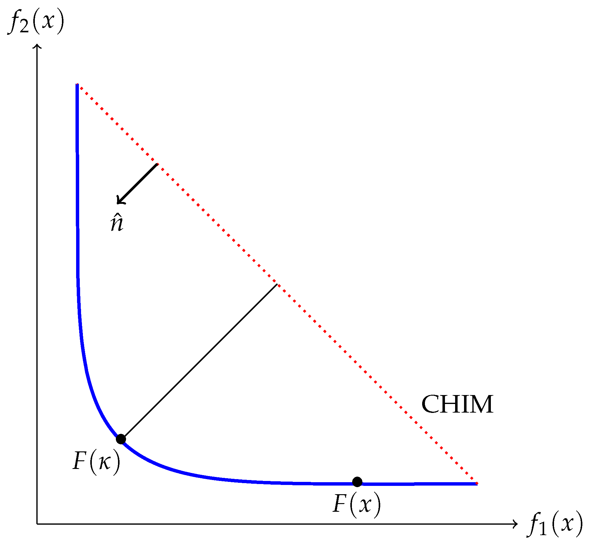
Figure 5 shows the Pareto front of a hypothetical BOP together with the image of a hypothetical starting point $x_0$. Since we are here focusing on the second phase of the Pareto Explorer, we are assuming that $x_0$ is Pareto optimal (and hence, that $F\left(x_0\right)$ is located on the Pareto front). The figure already indicates that the movement in objective space can be performed in order to compute a sequence of points leading toward knee solutions. More precisely, one can choose the “best fit” direction of $\widehat{n}$ that points along the linearized Pareto front at $F\left(x_0\right)$, and perform a movement into this direction. The question, however, in this context, is when to stop the search. In addition, for this problem, Figure 5 gives us a hint: denote by $\kappa ={(f_1\left(x^{*}\right),f_2\left(x^{*}\right))}^T$ the image of the solution $x^{*}$ of (16). Note that, at this point, the weight vector ${\widehat{\alpha }}_{\kappa }$ and the desired direction vector $d_y=\widehat{n}$ point into opposite direction. The following results shows that this is indeed the case, in general.

Theorem 2.

Let$x^{*}$be a KKT point of (1), and${\alpha }^{*}\in {\mathbb{R}}^k$be its associated Lagrange vector as specified in Theorem 1. Further, let$\widehat{n}$be the normal vector of the CHIM as specified in (16).

If${\alpha }^{*}$is anti-parallel to$\widehat{n}$, then there exist a vector${\beta }^{*}\in {\mathbb{R}}^k$and a value$t^{*}\in \mathbb{R}$such that the tuple$(x^{*},{\beta }^{*},t^{*})$is a KKT point of Problem (16).

Proof. 

If $(x^{*},{\beta }^{*},t^{*})$ is a KKT point of Problem (16) associated to the MOP (1), then there exist Lagrange multipliers $\overline{\lambda }={({\overline{\nu }}^T,{\overline{\alpha }}^T,{\tilde{\lambda }}^T)}^T\in {\mathbb{R}}^{k+k+p}$ and $\overline{\gamma }\in {\mathbb{R}}^{m+k}$, where $\overline{\nu }\in {\mathbb{R}}^k$, $\overline{\alpha }\in {\mathbb{R}}^k$, $\tilde{\lambda }\in {\mathbb{R}}^p$, and $\tilde{\gamma }\in {\mathbb{R}}^m$, such that the following conditions are satisfied:

$$\left(\begin{array}{c}0\\ 0\\ -1\end{array}\right)+\left(\begin{array}{c}0\\ \overline{\nu }\\ 0\end{array}\right)+\left(\begin{array}{c}J\left(x^{*}\right)\\ -\Phi \\ -{\widehat{n}}^T\end{array}\right)\overline{\alpha }+\sum _{i=1}^p\widetilde{{\lambda }_i}\left(\begin{array}{c}\nabla h_i\left(x^{*}\right)\\ 0\\ 0\end{array}\right)+\sum _{i=1}^m{\tilde{\gamma }}_i\left(\begin{array}{c}\nabla g_i\left(x^{*}\right)\\ 0\\ 0\end{array}\right)=0$$

(19)

$$\begin{array}{cc}\hfill e^T{\beta }^{*}-1=0& \end{array}$$

(20)

$$\begin{array}{cc}\hfill F\left(x^{*}\right)-\Phi {\beta }^{*}-t^{*}\widehat{n}-F^{*}=0& \end{array}$$

(21)

$$\begin{array}{cc}\hfill h_i(x^{*},{\beta }^{*},t^{*})=h_i\left(x^{*}\right)=0,& i=1\dots p,\end{array}$$

(22)

$$\begin{array}{cc}\hfill g_i(x^{*},{\beta }^{*},t^{*})=g_i\left(x^{*}\right)\le 0,& i=1\dots m,\end{array}$$

(23)

$$\begin{array}{cc}\hfill {\overline{\gamma }}_i\ge 0,& i=1\dots m,\end{array}$$

(24)

$$\begin{array}{cc}\hfill {\overline{\gamma }}_i{g}_i(x^{*},{\beta }^{*},t^{*})={\overline{\gamma }}_i{g}_i\left(x^{*}\right)=0,& i=1\dots m.\end{array}$$

(25)

We have to show that all of these equations are satisfied. For this, observe first that $x^{*}$ is a KKT point of (1), and hence, that $F\left(x^{*}\right)$ is located on the boundary of the image of the feasible region. Thus, by construction of the NBI subproblems there exist a vector ${\beta }^{*}\in {\mathbb{R}}^k$ and a value $t^{*}\in \mathbb{R}$ such that Equations (20) and (21) are satisfied. In addition, notice that conditions (5) and (6) are equivalent to (22) and (23), respectively (since $x^{*}$ is feasible). Further, when choosing $\overline{\gamma }=c\gamma$, where c is any positive scalar, we also have equivalence of conditions (9) and (10) with (24) and (25), respectively.

It remains to show that also condition (19) is satisfied for a vector $x^{*}$ that is a KKT point of (1) with ${\widehat{n}}^T\widehat{\alpha }=-1$.

Since $x^{*}$ satisfies (4), we have

$$\sum _{i=1}^k{\alpha }_i^{*}\nabla f_i\left(x^{*}\right)+\sum _{i=1}^p{\lambda }_i\nabla h_i\left(x^{*}\right)+\sum _{i=1}^m{\gamma }_i\nabla g_i\left(x^{*}\right)=0.$$

Choosing $c={{\displaystyle \frac{1}{\parallel \alpha \parallel }}}_2>0$ and multiplying the above equation by this value leads to

$$\sum _{i=1}^{k}c·{\alpha }_i^{*}\nabla f_i\left(x^{*}\right)+\sum _{i=1}^{p}c·{\lambda }_i\nabla h_i\left(x^{*}\right)+\sum _{i=1}^{m}c·{\gamma }_i\nabla g_i\left(x^{*}\right)=0.$$

(26)

We see that the first equation of (19) is satisfied when choosing $\overline{\alpha }=c·{\alpha }^{*}$, $\tilde{\lambda }=c·\lambda$, and $\tilde{\gamma }=c·\gamma$ (as already done before). If we choose $\overline{\nu }=\Phi \overline{\alpha }$, also the second equation of (19) is satisfied. It remains to show the third equation. Since ${\alpha }^{*}$ and $\widehat{n}$ are anti-parallel, it holds

$${\left(\frac{{\alpha }^{*}}{\parallel {\alpha }^{*}{\parallel }_2}\right)}^T\widehat{n}=-1$$

(note that $\widehat{n}$ is already normalized). Since $\overline{\alpha }={\alpha }^{*}/{\parallel {\alpha }^{*}\parallel }_2$ also this equation is satisfied, and the claim follows. □

3.3. The Algorithm

Based on the insights from the previous section, we are now in the position to adapt the Pareto Explorer to perform a movement from a given initial solution along the Pareto front toward a knee of the given MOP.

Assume we are given a Pareto optimal point $x_0$ of an equality constrained MOP (where inequalities that are active at $x_0$ are treated as equalities). That is, we can assume by Theorem 1 that there exist vectors ${\alpha }_0\in {\mathbb{R}}^k$ and ${\lambda }_0\in {\mathbb{R}}^p$ such that the tuple $(x_0,{\alpha }_0,{\lambda }_0)$ satisfies the KKT equations.

In order to compute a next candidate solution along the Pareto set/front, we see from Figure 5 that we can choose the “steering in objective space” of the Pareto Explorer as follows: the desired direction in objective space is given by the vector $\widehat{n}$ that is normal to the CHIM and that points toward the origin,

$$d_y=\widehat{n}.$$

(27)

Since this is not a feasible direction (note that $x_0$ is already optimal and all entries of $\widehat{n}$ are negative), we will in the next step have to compute the “best fit” direction that points along the Pareto front. To this end, we first compute the weight vector ${\alpha }_0$ associated to $x_0$. This can be done via solving the following scalar optimization problem, which follows directly from the KKT equations:

$$\underset{\alpha \in {\mathbb{R}}^k,\lambda \in {\mathbb{R}}^p}{min}\left\{{∥J^T\alpha +H^T\lambda ∥}_2^2:h\left(x\right)=0,{\alpha }_i\ge 0,i=1,\dots ,k,\sum _{i=1}^k{\alpha }_i=1\right\},$$

(28)

where $J=J\left(x\right)$ is as defined in (11), and

$$H=H\left(x\right)=\left(\begin{array}{c}\nabla h_1{\left(x\right)}^T\\ ⋮\\ \nabla h_p{\left(x\right)}^T\end{array}\right)\in {\mathbb{R}}^{p\times n}.$$

Since ${\alpha }_0$ is perpendicular to the linearized Pareto front at $F\left(x_0\right)$, we can obtain the desired search direction via an orthogonal projection of $d_y$ onto the orthogonal complement of ${\alpha }_0$. To get this vector, we first compute a $QR$-factorization of ${\alpha }_0$

$${\alpha }_0=Q_0{R}_0=(q_1^{\left(0\right)},\dots ,q_k^{\left(0\right)})R_0,$$

(29)

where $Q_0\in {\mathbb{R}}^{k\times k}$ is an orthogonal matrix and $R_0\in {\mathbb{R}}^{k\times 1}$ right upper triangular. The orthogonal complement of ${\alpha }_0$ is hence spanned by the column vectors of the matrix

$$B_0=(q_2^{\left(0\right)},\dots ,q_k^{\left(0\right)})\in {\mathbb{R}}^{k\times k-1},$$

(30)

and the orthogonal projection (and thus the best fit direction) is given by

$$d_y^{\left(0\right)}=B_0{B}_0^T{d}_y.$$

(31)

Next, we perform a step in direction $d_y^{\left(0\right)}$. Note that $d_y^{\left(0\right)}$ is defined in objective space. In order to realize such a movement, the respective direction in decision variable space is given by the vector ${\nu }_{d_0}\in {\mathbb{R}}^n$ that solves [49]:

$$\left(\begin{array}{cc}{W}_{\alpha ,\lambda }& H^T\\ H& 0\end{array}\right)\left(\begin{array}{c}{\nu }_{d_0}\\ y\end{array}\right)=\left(\begin{array}{c}-J^T{\mu }_{d_0}\\ 0\end{array}\right).$$

(32)

Hereby, $W_{\alpha ,\lambda }$ denotes the matrix

$$W_{\alpha ,\lambda }:=\sum _{i=1}^k{\alpha }_i{\nabla }^2{f}_i\left(x\right)+\sum _{i=1}^p{\lambda }_i{\nabla }^2{h}_i\left(x\right)\in {\mathbb{R}}^{n\times n},$$

(33)

and ${\mu }_{d_0}\in {\mathbb{R}}^n$ is the vector that solves

$$\left(\begin{array}{c}-J{W}_{\alpha }^{-1}{J}^T\\ e^T\end{array}\right){\mu }_{d_0}=\left(\begin{array}{c}{d}_0\\ 0\end{array}\right),$$

(34)

where $e={(1,\dots ,1)}^T\in {\mathbb{R}}^n$ and $d_0$ denotes–for sake of a simpler formulation—the direction vector $d_y^{\left(0\right)}$. The resulting search direction ${\nu }_{d_0}$ is tangential to the Pareto set at $x_0$. Alternatively, and as done in our implementations, one can use the matrix

$$W_{\alpha }:=\sum _{i=1}^k{\alpha }_i{\nabla }^2{f}_i\left(x\right)\in {\mathbb{R}}^{n\times n}$$

(35)

and solve the system

$$\left(\begin{array}{cc}{W}_{\alpha }& H^T\\ H& 0\end{array}\right)\left(\begin{array}{c}{\nu }_{d_0}\\ y\end{array}\right)=\left(\begin{array}{c}-J^T{\mu }_{d_0}\\ 0\end{array}\right).$$

(36)

to obtain ${\nu }_{d_0}$. The only difference of (36) compared to (32) is the use of $W_{\alpha }$ instead of $W_{\alpha ,\lambda }$ which saves the computations of the Hessians of the equality constraints, while still yielding satisfying results.

It remains to determine the step size. For this, we follow the suggestion of [42] and use

$$t_0=\frac{\tau }{\parallel J{\nu }_0{\parallel }_2},$$

(37)

such that, for the iterate

$${\tilde{x}}_1=x_0+t_0{\nu }_0,$$

(38)

it holds

$$\parallel F\left({\tilde{x}}_1\right)-F\left(x_0\right){\parallel }_2\approx \tau$$

(39)

for a user specified value of $\tau >0$. Note that ${\tilde{x}}_1$ is not necessarily a Pareto optimal solution. Since the aim is to perform a movement along Pareto set/front of the given MOP, the last step to obtain the new iterate $x_1$ is to compute a corrector step starting from ${\tilde{x}}_1$ which can, e.g., be realized via a multi-objective Newton method [30,53]. The Newton direction for at a point x for an equality constrained MOP can be obtained via solving the following problem:

$$\begin{array}{c}\hfill \underset{\nu \in {\mathbb{R}}^n,\delta \in \mathbb{R}}{min}\delta \\ \hfill \mathrm{s}.\mathrm{t}.& \nabla f_i{\left(x\right)}^T\nu +\frac{1}{2}{\nu }^T{\nabla }^2{f}_i\left(x\right)\nu \le \delta ,i=1,\dots ,k,\hfill \\ \hfill & h\left(x\right)+H^T\nu =0.\hfill \end{array}$$

(40)

Algorithm 1 shows the pseudo code of the complete algorithm to compute steps toward the knee solution. The basis is the above described iteration step. The process has to be stopped if either the corner of the Pareto front is reached since, or if the iterates are sufficiently close to the knee solution. Since the idea of the Pareto Explorer is to present all the steps to the decision-maker, a fixed step size $\tau$ is used as described above. At one point, however, an oscillatory behavior will be observed near to the knee solution since the value $\tau$ is not chosen adaptively. In order to address this issue, we start with one step size ${\tau }_1$. If a first oscillation occurs, the step size will be replaced with a smaller one, called ${\tau }_2$. The iteration will terminate if oscillation also occurs with this smaller step size. By Theorem 2, it also follows that a (local) knee solution is found if $d_y^{\left(i\right)}=0$, and that if $d_y^{\left(i\right)}$ is almost anti-parallel to $\widehat{n}$ one can expect that $x_i$ is near to such a solution. We hence have to stop the iteration in both cases (since the first case will never be observed in computations, we have left this step out in Algorithm 1).

Special attention has to be paid in case the algorithm is terminated since the iterates have reached a corner of the Pareto front (line 3 of Algorithm 1). If the Pareto front is concave, each corner point is indeed a knee solution. If the Pareto front is linear, then every point is a knee solution by definition. Hence, the algorithm will stop at $x_0$. Else (and if $x_0$ is not a corner solution), the corner will only be reached if an error occurred in the computation of $\widehat{n}$. This is the case if the MaOP is degenerated, which can be checked numerically via considering the condition number of the matrix $W_{\alpha }$: in case the Pareto front is degenerated at $x_i$, the matrix $W_{\alpha }=W_{\alpha }\left(x_i\right)$ is singular. In that case, the computation of the CHIM and the usage of the resulting direction vector $\widehat{n}$ makes no sense. Note, however, that the PE approach can be realized without explicitly computing the CHIM. Instead, it is necessary to define an alternative “suitable” direction vector. If, for instance, the values of each individual objective are more or less in the same range, one can choose the direction $d_y={(-1,\dots ,1)}^T$, and accordingly if the ranges differ. We will see examples for this in the next section.

Algorithm 1 Pareto Explorer for finding the knee.
Require:  $x_0$: initial Pareto optimal solution, $\widehat{n}$: normal vector of the CHIM, steps sizes ${\tau }_1>{\tau }_2>0$, tolerances ${ϵ}_1,{ϵ}_2$, maximal number M of iterations Ensure:  Set $\{x_1,\dots ,x_i\}$ of candidate solutions around $x_0$ in which images $F(x_i)$ are a best fit movement in $d_y$-direction along the Pareto front, where ideally $x_i$ is the knee solution. 1: $d_y:=\widehat{n}$ 2: $\tau :={\tau }_1$ 3: for$i=0,1,\dots ,M-1$do 4:     compute ${\alpha }_i$ as solution to (28) 5:     if $\parallel {\alpha }_i{\parallel }_{\infty }\ge 1-{ϵ}_2$ then
6:         return $\{x_1,\dots ,x_i\}$	▹ corner of Pareto front reached
7:     end if 8:     compute ${\alpha }_i=Q_i{R}_i=(q_1^{(i)},q_2^{(i)},\dots ,q_k^{(i)})R_i$ as in (29) 9:     set $B_i:=(q_2^{(i)},\dots ,q_k^{(i)})$ 10:     set $d_y^{(i)}:=B_i{B}_i^T\widehat{n}$ 11:     if $|\langle d_y^{(i)},d_y\rangle |\le {ϵ}_1$ then
12:         return $\{x_1,\dots ,x_i\}$         ▹ no further movement in $d_y$-direction can be performed (knee reached)
13:     end if
14:     if $sign({(d_y^{(i)})}_j)=-sign({(d_y^{(i-1)})}_j),\forall j=1,\dots ,k$ then	▹ oscillation of candidate solutions
15:         if $\tau ={\tau }_1$ then
16:            $\tau :={\tau }_2$	▹ reduce step size.
17:         else
18:            return $\{x_1,\dots ,x_i\}$	▹ oscillation with ${\tau }_2$ (knee reached)
19:         end if 20:     end if 21:     compute ${\mu }_{d_i}$ via solving (34) 22:     compute ${\nu }_i$ via solving (36) 23:     set $t_i:=\tau /{\parallel J{\nu }_i\parallel }_2$ 24:     set ${\tilde{x}}_{i+1}=x_i+t_i{\nu }_i$ 25:     compute solution $x_{i+1}$ of (1) near ${\tilde{x}}_{i+1}$ using a corrector step 26: end for
27: return$\{x_1,\dots ,x_M\}$	▹ more iterations needed to reach the knee

4. Numerical Results

In this section, we provide some numerical results in order to validate our proposal. We will further compare our method—as far as possible—to the original knee finding procedure proposed in Reference [41] via numerically solving Problem (16). To this end, we will first consider four academic benchmark test problems, and will then address a hypothetical scenario on a MaOP arising in plastic injection molding (PIM).

For all the experiments, we proceed as follows:

• For both methods, we use the normal $\widehat{n}$ of the CHIM of each problem. To compute the CHIM, the procedure fmincon of MATLAB is used. The cost for this step is reported, but it is not considered in the final analysis since both methods require $\widehat{n}$. CONDmathsizesmall denotes the condition number of $\Phi$ which a measure of how "close" the matrix is to be singular (and, in turn, how close the MOP is to be degenerated).
• We will use the same initial point $x_0$ for both methods.
• To solve (16), we
  • use ${\beta }^0={(1/k,\dots ,1/k)}^T\in {\mathbb{R}}^k$ and $t^0=0$ as initial values, and
  • report the number of function evaluations of F needed to solve the NBI problem. Note that this number can differ from the number of iterations of the NBI method since F is used in one of the constraints of (16).
• For the application of the PE, we proceed as specified in Algorithm 1, where
  • we specify the parameters ${\tau }_1>{\tau }_2>0$ for each problem,
  • we use the same tolerances as those employed for the NBI method, and
  • we use the BFGS variant of PE, that is, we approximate the Hessians via the BFGS method. We report separately how many Jacobians were needed. We also report the total number of function evaluations that PE needs considering that Automatic Differentiation [54] is used. Doing so, each Jacobian evaluation counts as four function calls.
• We compute and compare the distances t obtained by the two algorithms. For this, we will
  • denote the distance to the approximated CHIMs by $t_a^{*}$, and
  • denote the distance to the exact CHIMs (which are known for the academic benchmark functions) by $t_r^{*}$.

4.1. MOP (14)

For illustration purposes, we start with two three-objective problems. The first one we consider is the three-objective problem that is defined in Equation (14). For this problem, the cost for the approximation of the CHIM has been 10 function evaluations. The condition number of the CHIM is COND = 4.5140 (i.e., well-conditioned). That is, the approximated CHIM is basically identical to the real one.

As the initial solution, we choose $x_0:={\displaystyle \frac{a^{\left(1\right)}+a^{\left(3\right)}}{2}}$.

Table 1. Computational cost for multi-objective optimization problem (MOP) (14).

	Stage	# S	# F	# J	${\mathit{t}}_{\mathit{a}}^{*}$	${\mathit{t}}_{\mathit{r}}^{*}$
	${\tau }_1=1.5$	7	11	11	4.236854	4.236854
PE	${\tau }_2=0.05$	6	10	10	4.242638	4.242638
	Total ${}^{\star }$		21	21
NBI		–	84	–	4.242640	4.242640

${}^{\star }$ 21 + 4(21) = 105 function evaluations considering AD.

and Figure 6 show the numerical results obtained for PE and NBI.

Both methods yield essentially the same solution, and the overall cost (measured in calls of F) is around 20 percent less for NBI. On the other hand, as designed, NBI only delivers the knee solution, while PE delivers (also as designed) 6 solutions that lead from $x_0$ toward the knee solution with $\parallel F\left(x_i\right)-F\left(x_{i-1}\right){\parallel }_2\approx {\tau }_1$. The decision-maker is hence given more options that are in this case equally distributed along the Pareto front. Any of these further solutions may be of interest, for instance, for the case that the knee solution is “too far” away from the initial solution $x_0$, respectively, the objective values are “too far” from $F\left(x_0\right)$.

4.2. MOP (17)

The next problem we consider is the three-objective problem (17). We needed 83 function evaluations to obtain an approximation of the CHIM with COND= 4.5142 (actually, the CHIM of this problem is identical to the one of MOP (14)). That is, we again obtain a nearly perfect accuracy. We used the same initial condition and values for ${\tau }_i$ as for the previous problem.

Table 2. Numerical results for MOP (17).

	Stage	# S	# F	# J	${\mathit{t}}_{\mathit{a}}^{*}$	${\mathit{t}}_{\mathit{r}}^{*}$
	${\tau }_1=2.2$	5	13	12	3.112989	3.112989
PE	${\tau }_2=0.02$	10	17	16	3.125253	3.125253
	Total ${}^{\star }$		30	28
NBI		–	112	–	3.125279	3.125279

${}^{\star }$ 30 + 4(28) = 141 function evaluations considering AD.

and Figure 7 show the numerical results and the cost for both methods. NBI is capable of detecting the knee solution in this case due to the change of the formulation in the problem. Further, similar as for the above problem, both methods find the same solution while NBI needs less function evaluations. The consideration of the cost, however, changes if one only considers the PE results for the first step size ${\tau }_1$. The radar chart and the line plot in Figure 7 show that the final solution obtained via using ${\tau }_1$ is already very close to the actual knee solution. The last changes may not be that important for a decision-maker. When counting only the steps for ${\tau }_1$, PE needed $13+4·12=61$ functions evaluations, i.e., the half of what NBI needed to obtain the knee solution (albeit with higher accuracy).

4.3. Problem minDTLZ2

Our next test problem is the problem minDTLZ2 [55], which is scalable both in the number of decision variables and the objectives. We have chosen to take $n=30$ and $k=10$ for our computations. The cost for the approximation of the CHIM was 1139 function evaluations, yielding COND = $1.0169$—that is, also in this case the approximation quality of the CHIM is very good.

Table 3. Numerical results for minDTLZ2.

	Stage	# S	# F	# J	${\mathit{t}}_{\mathit{a}}^{*}$	${\mathit{t}}_{\mathit{r}}^{*}$
	${\tau }_1=0.5$	15	16	16	4.227605	4.257558
PE	${\tau }_2=0.02$	25	26	26	4.245430	4.273449
	Total ${}^{\star }$		41	41
NBI		–	1653	–	4.244890	4.272937

${}^{\star }$ 41 + 4(41) = 210 function evaluations considering AD.

and Figure 8 show the numerical results of both methods. Hereby, we have taken $x_0=x_1^{*}$, i.e., the minimizer of $f_1$ (which is known from the computation of the CHIM) as starting point. Again, both methods obtain in principle the same solution; however, this time, the computational cost is much less for PE, while this method even computed 15 different solutions that are of potential use for the decision-maker. To obtain the final solution, PE needed around 10 percent of the function calls that were needed for NBI, which is due to the fact that a higher dimensional problem is considered. When only counting the solutions for ${\tau }_1$, PE only needed 16 + 16 × 4 = 80 function calls, which is equivalent to only around 5 percent of the cost for the NBI method.

From our previous experiment, we observe that the performance of the PE improves, compared to the NBI method, when the number of objectives increases. In order to further illustrate this fact, we consider the same problem but change the number of objectives; in particular, we will consider $k=3,4,\dots ,22$ and $n=3k$. For this new experiment, we also take $x_0=x_1^{*}$, and we fix the values ${\tau }_1=0.5$ and ${\tau }_2=0.02$ for all the PE executions. Finally, as we know that this problem is symmetric, we consider the direction $d_y:={(1,\dots ,1)}^T\in {\mathbb{R}}^k$ as the steering direction for PE. In summary, we obtain the numerical results that are displayed in

Table 4. Numerical results for the minDTLZ2 for different values of k.

					PE
	NBI				${\mathit{\tau }}_{\mathbf{1}}$				${\mathit{\tau }}_{\mathbf{2}}$				Total
$\mathit{k}$	# ${\mathit{F}}_{\mathit{CHIM}}$	# $\mathit{F}$	time (s)	${\mathit{t}}_{\mathit{nbi}}$	# S	# $\mathit{F}$	#$\mathit{J}$	${\mathit{t}}_{{\mathit{\tau }}_{\mathbf{1}}}$	# S	# $\mathit{F}$	#$\mathit{J}$	${\mathit{t}}_{{\mathit{\tau }}_{\mathbf{2}}}$	time (s)	# $\mathit{F}$
3	228	283	0.143478	1.154347	6	7	7	1.150788	15	17	17	1.154569	0.271545	120
4	332	470	0.202298	1.616918	8	9	9	1.582242	33	35	35	1.617166	0.471207	220
5	398	508	0.272306	2.065890	9	10	10	2.049299	28	30	30	2.065911	0.439411	200
6	511	760	0.376826	2.508848	10	11	11	2.500748	25	27	27	2.508853	0.438211	190
7	671	966	0.549365	2.949400	11	12	12	2.946009	22	24	24	2.949854	0.496617	180
8	776	1127	0.742522	3.389544	12	13	13	3.388383	20	22	22	3.390068	0.403380	175
9	959	1259	1.031438	3.829831	14	15	15	3.814151	37	39	39	3.830407	0.752654	270
10	1139	1653	1.308785	4.270679	15	16	16	4.254194	40	42	42	4.271297	0.977876	290
11	1219	2036	1.558900	4.712335	16	17	17	4.696036	42	44	44	4.713017	1.096160	305
12	1407	1769	1.964145	5.155558	17	18	18	5.140185	42	44	44	5.155735	1.126582	310
13	1432	2558	2.265293	5.598770	18	19	19	5.586221	42	44	44	5.599621	1.201590	315
14	1519	2811	2.653185	6.043542	21	22	22	6.032265	45	47	47	6.044458	1.313640	345
15	1676	3187	3.198856	6.489327	20	21	21	6.479375	44	46	46	6.490333	1.456578	335
16	1837	3656	3.818040	6.936143	21	22	22	6.926772	45	47	47	6.937242	1.806661	345
17	1926	3812	4.368855	7.383958	22	23	23	7.374801	46	48	48	7.385169	2.023789	355
18	1954	4486	4.901236	7.832741	23	24	24	7.823462	48	50	50	7.834042	2.384949	370
19	2099	4881	5.772514	8.282457	24	25	25	8.273021	50	52	52	8.283846	2.747111	385
20	2219	5380	6.639668	8.733055	25	26	26	8.724442	50	52	52	8.734563	3.037196	390
21	2276	5130	7.526548	9.184532	26	27	27	9.177164	51	53	53	9.186110	3.314400	400
22	2411	7117	8.922805	9.636838	27	28	28	9.630991	50	52	52	9.638511	2.995077	400

, which also show the CPU times used for the execution of each algorithm. Figure 9 shows the PE results for $k=6,15$ and 22. As it can be seen, PE needs less function evaluations in all cases (while generating an entire path of solutions toward the knee solution, and not “only” the knee), and the difference gets even more significant with increasing value of k.

4.4. Problem C-convDTLZ2

Our last benchmark problem we consider here is the following one, which we will call C-convDTLZ2:

$$\begin{array}{cc}\hfill & {\displaystyle \underset{x\in {\mathbb{R}}^n}{min}F\left(x\right)={({\tilde{f}}_1\left(x\right),\dots ,{\tilde{f}}_k\left(x\right))}^T,}\hfill \\ \hfill \mathrm{s}.\mathrm{t}.& \\ \hfill & {\displaystyle \sum _{i=1}^{k-1}{(x_i-0.5)}^2=0.25}\hfill \\ \hfill & 0\le x_i\le 1,i=1,\dots ,n,\hfill \end{array}$$

(41)

where

$$\begin{array}{cc}\hfill {\tilde{f}}_j\left(x\right)& =f_j{\left(x\right)}^4,j=1,\dots k-1\hfill \\ \hfill {\tilde{f}}_k\left(x\right)& =f_k{\left(x\right)}^2\hfill \\ \hfill f_i\left(x\right)& =\left(1+g\left(x\right)\right)sin\left(0.5\pi x_{k-1}\right)\prod _{i=1}^{k-i}cos\left(0.5\pi x_i\right),\hfill \\ \hfill g\left(x\right)& =\sum _{i=k}^n{(x_i-0.5)}^2.\hfill \end{array}$$

(42)

The problem is a modification of convDTLZ2 [48], where we have added an equality constraint so that the dimension of the Pareto front is $k-2$. More precisely, the Pareto front of convDTLZ2 is connected and convex. The front of C-convDTLZ2 is given by the $k-2$ dimensional border of this set. Further, the objective $f_k$ does not have a unique minimum. We have chosen here to take $n=10$ decision variables and $k=5$ objectives for our computations.

We first perform the same computations, as for the previous examples. We needed 340 function evaluations to compute the CHIM yielding COND = $1.2162\times {10}^3$. We only present the result of one CHIM we have obtained (in particular, we used one minimizer of $f_5$ found by fmincon), results using further approximations—which are not presented here—-confirmed the results which are shown in

Table 5. Numerical results for the first run with the C-convDTLZ2.

	Stage	# S	# F	# J	${\mathit{t}}_{\mathit{a}}^{*}$	${\mathit{t}}_{\mathit{r}}^{*}$
	${\tau }_1=0.75$	5	918	211	0.095552	0.702722
PE ${}^{\star }$	${\tau }_2=0.01$	–	–	–	–	–
NBI		–	3524	–	2.250934	17.020339

${}^{\star }$ Total of 918 + 4(211) = 1762 function evaluations considering AD.

and Figure 10. For this, we have chosen $x_0={(0.75,0.75,0.75,0.75,0.52,0.52,0.52,0.52,0.52,0.52)}^T$ as starting solution. The objective value obtained by NBI is given by ${(0,0,0,0,39.0586)}^T$, and the respective objective value for PE is ${(0,0,0,0,2.5713)}^T$. At first sight, it seems that the NBI result is much better than the one obtained by PE. However, none of the obtained solutions are knee points since one corner of the Pareto front is ${(0,0,0,0,1)}^T$. Consequently, both obtained solutions are in fact only weakly optimal. The PE method has been terminated since a corner point has been detected (up to the given precision). In addition, the values for the condition numbers of the matrices $W_{\alpha }$ have been up to $1.0\times {10}^{14}$ during the search. PE could hence detect that this result is meaningless.

In a next step, we have applied PE again but now without using the direction $\widehat{n}$ that results from the CHIM. Since the objective values for all objectives seem to be in the same range, we have next used the direction $d_y={(-1,\dots ,-1)}^T$. For sake of a comparison, we have also applied the NBI method, where have used the same CHIM as above, but there we have replaced the normal $\widehat{n}$ by $d_y$.

Table 6. Numerical results for the second run with the C-convDTLZ2.

	Stage	# S	# F	# J	${\mathit{t}}_{\mathit{r}}^{*}$
	${\tau }_1=0.75$	5	6339	1120	0.054672
PE	${\tau }_2=0.01$	1	24	17	0.054672
	Total ${}^{\star }$		6339	1137
NBI		–	2818	–	17.021602

${}^{\star }$ 6339 + 4(1137) = 10887 function evaluations considering AD.

and Figure 11 show the respective results. The NBI method again computes a weakly optimal solution which is not globally optimal. This time, however, the PE is capable of detecting a KKT point of (16). The relatively high cost of the method results from the degeneracy of the considered MaOP. The used continuation method is yet not tuned for the treatment of degenerated problems, which we have to leave for future work. Nevertheless, unlike NBI, it is able to detect the solution (and even a path to it), which may be helpful in the decision-making process.

4.5. Plastic Injection Molding

As the last example, we consider a many objective problem that arises in the design of plastic injection molding (PIM) processes. More precisely, as case study, we use the model of the design of a particular plastic gear as reported in Reference [56]. The problem can be written as

$$\begin{array}{c}\hfill \begin{array}{cc}\hfill {\displaystyle \underset{x\in {\mathbb{R}}^4}{min}}& F\left(x\right)={(f_1\left(x\right),\dots ,f_7\left(x\right))}^T,\hfill \\ \hfill \mathrm{s}.\mathrm{t}& 190\le x_1\le 230\hfill \\ & 3\le x_2\le 5\hfill \\ & 60\le x_3\le 100\hfill \\ & 8\le x_4\le 14.\hfill \end{array}\end{array}$$

(43)

The four parameters of the problem are the melt temperature ($x_1$), the packing time ($x_2$), the packing pressure ($x_3$), and the cooling time ($x_7$). The problem as seven objectives. Cosmetic characteristics are measured by the warpage ($f_1$) in the product, shrinkage ($f_2$) and sink marks ($f_3$). Functional properties are represented by residual stresses, such as Von Mises ($f_4$) and shear stresses ($f_5$). Productivity is measured by the cycle time ($f_6$) and the clamping force ($f_7$).

A numerical approximation of the CHIM led to the condition number COND $=1.2087\times {10}^{04}$. We have hence omitted to apply the NBI method. Instead, we only apply PE to this problem using the direction vector

$$d_y:={(min\left(f_1\right)-max\left(f_1\right),\dots ,min\left(f_7\right)-max\left(f_7\right))}^T\in {\mathbb{R}}^7,$$

(44)

where we have taken the minimal and maximal value according to each objective out of a given sample set. As the initial point, we have chosen $x_0:={(230.00,5.00,94.73,13.87)}^T$, which is taken from Reference [56]. For PE, we used the step sizes ${\tau }_1=0.5$ and ${\tau }_2:=0.05$. Figure 12 shows the graphical result of the method. In summary, we obtained a path of 30 different solutions that led to the knee solution for this problem. For this, 30 function evaluations and 30 Jacobians had to be evaluated (leading to a cost of 150 function evaluations when using A.D.). As it can be seen, the movement has been performed according to the desired direction in objective space. Though the entire path of solutions has been computed (and presented), the decision-maker can of course choose at any time either to accept a computed candidate solution, or to change the direction in which the steering has to be performed.

5. Discussion

The solution sets of given multi- and many objective optimization problems typically form ($k-1$)-dimensional objects, where k is the number of objectives involved in such a problem. Hence, these Pareto sets and fronts cannot be computed or adequately presented to the decision-maker anymore for problems with more than, say, $k=4$ objectives. Knee solutions are preferred by many decision-makers since these solutions represent (at least locally) the best trade-offs between the different conflicting objectives.

In this work, we addressed the knee points as defined by Das. For this, we first (slightly) modified its definition. For its original definition, the author had problems with few objectives in mind where the knee solutions are indeed typically near to the “center” of the Pareto front. For problems with more objectives and/or degenerated problems (i.e., problems where the dimension of the Pareto set/front is less than $k-1$), this does not have to be the case. We, therefore, think that the new definition is better suited, in particular, for many objective optimization problems.

In a next (and main) step, we adapted the Pareto Explorer to perform a movement along the Pareto set/front toward knee solutions. To this end, we first characterized the knee solution in Section 3.2 and, based on this, proposed a modification of the second phase of the Pareto Explorer to perform a local movement along the Pareto set/front of a given multi- and many objective optimization problem toward knee solutions. We demonstrated the usefulness of the method on several examples. Further, we made a comparison to the method of Das, as far as it was possible. The results show that the continuation-like strategy is beneficial, in particular, for problems with an increasing number of decision variables and objectives. Moreover, the PE approach seems to be affected less by the approximation quality of the CHIM and the normal vector $\widehat{n}$. For multi-modal problems, the approximation of the CHIM is always an issue, and, for degenerated problems, the normal vector is not uniquely defined anymore. For such problems, the PE approach could be taken as an alternative, which we showed in two examples. Note, however, the aim of the PE is to present a path of solutions that are uniformly distributed along the Pareto front. The adaptation of the PE to solely compute the knee solution was been addressed here. Further investigations in this direction may be part of future work. Another interesting aspect would be to adapt the continuation strategy Pareto Tracer to degenerated problems, which is also out of the scope of this work.

References

1. Peitz, S.; Dellnitz, M. A Survey of Recent Trends in Multiobjective Optimal Control—Surrogate Models, Feedback Control and Objective Reduction. Math. Comput. Appl. 2018, 23, 30. [Google Scholar] [CrossRef] [Green Version]
2. Moghadam, M.E.; Falaghi, H.; Farhadi, M. A Novel Method of Optimal Capacitor Placement in the Presence of Harmonics for Power Distribution Network Using NSGA-II Multi-Objective Genetic Optimization Algorithm. Math. Comput. Appl. 2020, 25, 17. [Google Scholar]
3. Aguilera-Rueda, V.J.; Cruz-Ramírez, N.; Mezura-Montes, E. Data-Driven Bayesian Network Learning: A Bi-Objective Approach to Address the Bias-Variance Decomposition. Math. Comput. Appl. 2020, 25, 37. [Google Scholar] [CrossRef]
4. Yi, J.H.; Deb, S.; Dong, J.; Alavi, A.H.; Wang, G.G. An improved NSGA-III algorithm with adaptive mutation operator for Big Data optimization problems. Future Gener. Comput. Syst. 2018, 88, 571–585. [Google Scholar] [CrossRef]
5. Wang, G.; Cai, X.; Cui, Z.; Min, G.; Chen, J. High Performance Computing for Cyber Physical Social Systems by Using Evolutionary Multi-Objective Optimization Algorithm. IEEE Trans. Emerg. Top. Comput. 2020, 8, 20–30. [Google Scholar] [CrossRef]
6. Deb, K. Multi-Objective Optimization Using Evolutionary Algorithms; John Wiley & Sons: Chichester, UK, 2001. [Google Scholar]
7. Coello Coello, C.A.; Lamont, G.B.; Van Veldhuizen, D.A. Evolutionary Algorithms for Solving Multi-Objective Problems, 2nd ed.; Springer: New York, NY, USA, 2007. [Google Scholar]
8. Dellnitz, M.; Schütze, O.; Hestermeyer, T. Covering Pareto Sets by Multilevel Subdivision Techniques. J. Optim. Theory Appl. 2005, 124, 113–155. [Google Scholar] [CrossRef]
9. Sun, J.Q.; Xiong, F.R.; Schütze, O.; Hernández, C. Cell Mapping Methods—Algorithmic Approaches and Applications; Springer: Berlin/Heidelberg, Germany, 2019. [Google Scholar]
10. Hernández, C.I.; Schütze, O.; Sun, J.Q.; Ober-Blöbaum, S. Non-Epsilon Dominated Evolutionary Algorithm for the Set of Approximate Solutions. Math. Comput. Appl. 2020, 25, 3. [Google Scholar] [CrossRef] [Green Version]
11. Bogoya, J.M.; Vargas, A.; Schütze, O. The Averaged Hausdorff Distances in Multi-Objective Optimization: A Review. Mathematics 2019, 7, 894. [Google Scholar] [CrossRef] [Green Version]
12. Cuate, O.; Ponsich, A.; Uribe, L.; Zapotecas, S.; Lara, A.; Schütze, O. A New Hybrid Evolutionary Algorithm for the Treatment of Equality Constrained MOPs. Mathematics 2020, 8, 7. [Google Scholar] [CrossRef] [Green Version]
13. Cheng, C.; Lin, S.; Pourhejazy, P.; Ying, K.; Li, S.; Liu, Y. Greedy-Based Non-Dominated Sorting Genetic Algorithm III for Optimizing Single-Machine Scheduling Problem With Interfering Jobs. IEEE Access 2020, 8, 142543–142556. [Google Scholar] [CrossRef]
14. Yi, J.H.; Xing, L.N.; Wang, G.G.; Dong, J.; Vasilakos, A.V.; Alavi, A.H.; Wang, L. Behavior of crossover operators in NSGA-III for large-scale optimization problems. Inf. Sci. 2020, 509, 470–487. [Google Scholar] [CrossRef]
15. Sun, J.; Miao, Z.; Gong, D.; Zeng, X.; Li, J.; Wang, G. Interval Multiobjective Optimization With Memetic Algorithms. IEEE Trans. Cybern. 2020, 50, 3444–3457. [Google Scholar] [CrossRef] [PubMed]
16. Ishibuchi, H.; Sakane, Y.; Tsukamoto, N.; Nojima, Y. Evolutionary Many-Objective Optimization by NSGA-II and MOEA/D with Large Populations. In Proceedings of the IEEE International Conference on Systems, Man and Cybernetics (SMC 2009), San Antonio, TX, USA, 11–14 October 2009; pp. 1758–1763. [Google Scholar]
17. Singh, H.K.; A, I.; Ray, T. A Pareto Corner Search Evolutionary Algorithm and Dimensionality Reduction in Many-Objective Optimization Problems. IEEE Trans. Evol. Comput. 2011, 15, 539–556. [Google Scholar] [CrossRef]
18. López Jaimes, A.; Coello Coello, C.A.; Chakraborty, D. Objective Reduction Using a Feature Selection Technique. In Proceedings of the 10th Annual Conference on Genetic and Evolutionary Computation, GECCO ’08, Atlanta, GA, USA, 12–16 July 2008; Association for Computing Machinery: New York, NY, USA, 2008; pp. 673–680. [Google Scholar] [CrossRef]
19. López Jaimes, A.; Coello, C.A.C.; Urías Barrientos, J.E. Online Objective Reduction to Deal with Many-Objective Problems. In Evolutionary Multi-Criterion Optimization; Ehrgott, M., Fonseca, C.M., Gandibleux, X., Hao, J.K., Sevaux, M., Eds.; Springer: Berlin/Heidelberg, Germany, 2009; pp. 423–437. [Google Scholar]
20. Zhang, Y.; Wang, G.G.; Li, K.; Yeh, W.C.; Jian, M.; Dong, J. Enhancing MOEA/D with information feedback models for large-scale many-objective optimization. Inf. Sci. 2020, 522, 1–16. [Google Scholar] [CrossRef]
21. Gu, Z.M.; Wang, G.G. Improving NSGA-III algorithms with information feedback models for large-scale many-objective optimization. Future Gener. Comput. Syst. 2020, 107, 49–69. [Google Scholar] [CrossRef]
22. Gass, S.; Saaty, T. The computational algorithm for the parametric objective function. Nav. Res. Logist. Q. 1955, 2, 39–45. [Google Scholar] [CrossRef]
23. Mavrotas, G. Effective implementation of the ϵ-constraint method in Multi-Objective Mathematical Programming problems. Appl. Math. Comput. 2009, 213, 455–465. [Google Scholar] [CrossRef]
24. Steuer, R.E.; Choo, E.U. An Interactive Weighted Tchebycheff Prodecure for Multiple Objective Progamming. Math. Program. 1983, 26, 326–344. [Google Scholar] [CrossRef]
25. Wierzbicki, A.P. A mathematical basis for satisficing decision-making. Math. Model. 1982, 3, 391–405. [Google Scholar] [CrossRef] [Green Version]
26. Bogetoft, P.; Hallefjord, A.; Kok, M. On the convergence of reference point methods in multiobjective programming. Eur. J. Oper. Res. 1988, 34, 56–68. [Google Scholar] [CrossRef]
27. Hernández-Mejía, A.; Schütze, O.; Cuate, O.; Lara, A.; Deb, K. RDS-NSGA-II: A Memetic Algorithm for Reference Point Based Multi-objective Optimization. Eng. Optim. 2017, 49, 828–845. [Google Scholar] [CrossRef]
28. Miettinen, K. Nonlinear Multiobjective Optimization; Springer Science & Business Media: Berlin/Heidelberg, Germany, 2012; Volume 12. [Google Scholar]
29. Ehrgott, M. Multicriteria Optimization; Springer: Berlin/Heidelberg, Germany, 2005. [Google Scholar]
30. Schütze, O.; Cuate, O.; Martín, A.; Peitz, S.; Dellnitz, M. Pareto Explorer: A global/local exploration tool for many-objective optimization problems. Eng. Optim. 2019, 52, 832–855. [Google Scholar] [CrossRef]
31. Branke, J.; Deb, K.; Dierolf, H.; Osswald, M. Finding Knees in Multi-Objective Optimization. In Parallel Problem Solving from Nature—PPSN VIII; Lecture Notes in Computer Science Volume 3242; Springer: Birmingham, UK, 2004; pp. 722–731. [Google Scholar]
32. Schütze, O.; Laumanns, M.; Coello Coello, C.A. Approximating the Knee of an MOP with Stochastic Search Algorithms. In Parallel Problem Solving from Nature–PPSN X; Lecture Notes in Computer Science Volume 5199; Rudolph, G., Jansen, T., Lucas, S., Poloni, C., Beume, N., Eds.; Springer: Dortmund, Germany, 2008; pp. 795–804. [Google Scholar]
33. Bechikh, S.; Said, L.B.; Ghédira, K. Searching for Knee Regions in Multi-objective Optimization using Mobile Reference Points. In Proceedings of the 25th Annual ACM Symposium on Applied Computing (SAC’2010), Sierre, Switzerland, 22–26 May 2010; ACM Press: Sierre, Switzerland, 2010; pp. 1118–1125. [Google Scholar]
34. Shukla, P.K.; Braun, M.A.; Schmeck, H. Theory and Algorithms for Finding Knees. In Evolutionary Multi-Criterion Optimization, Proceedings of the 7th International Conference, EMO 2013, Sheffield, UK, 19–22 March 2013; Lecture Notes in Computer Science Volume 7811; Purshouse, R.C., Fleming, P.J., Fonseca, C.M., Greco, S., Shaw, J., Eds.; Springer: Sheffield, UK, 2013; pp. 156–170. [Google Scholar]
35. Recio, G.; Deb, K. Solving Clustering Problems Using Bi-Objective Evolutionary Optimisation and Knee Finding Algorithms. In Proceedings of the 2013 IEEE Congress on Evolutionary Computation (CEC’2013), Cancun, Mexico, 20–23 June 2013; IEEE Press: Cancun, Mexico, 2013; pp. 2848–2855. [Google Scholar]
36. Du, W.; Leung, S.Y.S.; Kwong, C.K. Time series forecasting by neural networks: A knee point-based multiobjective evolutionary algorithm approach. Expert Syst. Appl. 2014, 41, 8049–8061. [Google Scholar] [CrossRef]
37. Sudeng, S.; Wattanapongsakorn, N. A Decomposition-Based Approach for Knee Solution Approximation in Multi-Objective Optimization. In Proceedings of the 2016 IEEE Congress on Evolutionary Computation (CEC’2016), Vancouver, BC, Canada, 24–29 July 2016; IEEE Press: Vancouver, BC, Canada, 2016; pp. 3710–3717. [Google Scholar]
38. Maltese, J.; Ombuki-Berman, B.M.; Engelbrecht, A.P. Pareto-Based Many-Objective Optimization Using Knee Points. In Proceedings of the 2016 IEEE Congress on Evolutionary Computation (CEC’2016), Vancouver, BC, Canada, 24–29 July 2016; IEEE Press: Vancouver, BC, Canada, 2016; pp. 3678–3686. [Google Scholar]
39. Li, Y.; Li, Y. Two-Step Many-Objective Optimal Power Flow Based on Knee Point-Driven Evolutionary Algorithm. Processes 2018, 6, 250. [Google Scholar] [CrossRef] [Green Version]
40. Li, W.; Wang, R.; Zhang, T.; Ming, M.; Li, K. Reinvestigation of evolutionary many-objective optimization: Focus on the Pareto knee front. Inf. Sci. 2020, 522, 193–213. [Google Scholar] [CrossRef]
41. Das, I. On characterizing the “knee” of the Pareto curve based on Normal-Boundary Intersection. Struct. Optim. 1999, 18, 107–115. [Google Scholar] [CrossRef]
42. Hillermeier, C. Nonlinear Multiobjective Optimization: A Generalized Homotopy Approach; Springer: Berlin/Heidelberg, Germany, 2001; Volume 135. [Google Scholar]
43. Karush, W. Minima of Functions of Several Variables With Inequalities as Side Constraints. Master’s Thesis, Department of Mathematics, University of Chicago, Chicago, IL, USA, 1939. [Google Scholar]
44. Kuhn, H.W.; Tucker, A.W. Nonlinear programming. In Proceedings of the Second Berkeley Symposium on Mathematical Statistics and Probability, Berkeley, CA, USA, 31 July–12 August 1950; University of California Press: Los Angeles, CA, USA, 1951; pp. 481–492. [Google Scholar]
45. Deb, K.; Pratap, A.; Agarwal, S.; Meyarivan, T. A fast and elitist multiobjective genetic algorithm: NSGA-II. Evol. Comput. IEEE Trans. Evol. Comput. 2002, 6, 182–197. [Google Scholar] [CrossRef] [Green Version]
46. Beume, N.; Naujoks, B.; Emmerich, M. SMS-EMOA: Multiobjective selection based on dominated hypervolume. Eur. J. Oper. Res. 2007, 181, 1653–1669. [Google Scholar] [CrossRef]
47. Lara, A.; Sanchez, G.; Coello Coello, C.A.; Schütze, O. HCS: A new local search strategy for memetic multiobjective evolutionary algorithms. IEEE Trans. Evol. Comput. 2009, 14, 112–132. [Google Scholar] [CrossRef]
48. Deb, K.; Jain, H. An evolutionary many-objective optimization algorithm using reference-point-based nondominated sorting approach, part I: Solving problems with box constraints. Trans. Evol. Comput. 2014, 18, 577–601. [Google Scholar] [CrossRef]
49. Martin, A.; Schütze, O. Pareto Tracer: A predictor–corrector method for multi-objective optimization problems. Eng. Opt. 2018, 50, 516–536. [Google Scholar]
50. Das, I.; Dennis, J.E. Normal-boundary intersection: A new method for generating the Pareto surface in nonlinear multicriteria optimization problems. SIAM J. Opt. 1998, 8, 631–657. [Google Scholar] [CrossRef] [Green Version]
51. Kim, J.; Kim, S.K. A CHIM-based interactive Tchebycheff procedure for multiple objective decision-making. Comput. Oper. Res. 2006, 33, 1557–1574. [Google Scholar] [CrossRef]
52. Messac, A.; Mattson, C.A. Normal constraint method with guarantee of even representation of complete Pareto frontier. AIAA J. 2004, 42, 2101–2111. [Google Scholar] [CrossRef] [Green Version]
53. Fliege, J.; Drummond, L.M.G.; Svaiter, B.F. Newton’s Method for Multiobjective Optimization. SIAM J. Opt. 2009, 20, 602–626. [Google Scholar] [CrossRef] [Green Version]
54. Griewank, A.; Walther, A. Evaluating Derivatives: Principles and Techniques of Algorithmic Differentiation; Siam: Philadelphia, PA, USA, 2008; Volume 105. [Google Scholar]
55. Ishibuchi, H.; Setoguchi, Y.; Masuda, H.; Nojima, Y. Performance of Decomposition-Based Many-Objective Algorithms Strongly Depends on Pareto Front Shapes. IEEE Trans. Evol. Comput. 2017, 21, 169–190. [Google Scholar] [CrossRef]
56. Alvarado-Iniesta, A.; Cuate, O.; Schütze, O. Multi-objective and many objective design of plastic injection molding process. Int. J. Adv. Manuf. Technol. 2019, 102, 3165–3180. [Google Scholar]
Figure 1. Pareto front of a hypothetical bi-objective problem with knee solution κ .
Mathematics 08 01651 g001
Figure 2. (a) d y ( i ) is the orthogonal projection of d y onto the linearized Pareto front at F ( x i ) and hence the best fit direction for a movement along the Pareto front. (b) The process has to be stopped at x f if T y f F ( M ) and d y are orthogonal to each other.
Mathematics 08 01651 g002
Figure 3. Example where the normal-boundary intersection (NBI)method is not able to get a good approximation to the entire Pareto front.
Mathematics 08 01651 g003
Figure 4. Example of a three-objective problem where the knee solutions defined by (12) and (16) differ.
Mathematics 08 01651 g004
Figure 5. Illustrative example of the use of Pareto Explorer (PE) to find the knee. Here, we start the steering in objective space at the point x 0 (which has α ^ 0 ) in the direction d y : = n ^ . We compute a sequence of points until the stop criterion (a) is satisfied, i.e., the knee κ = ( f 1 ( x * ) , f 2 ( x * ) ) T . Notice that α ^ κ (associated to x * ) is in the opposite direction of n ^ .
Mathematics 08 01651 g005
Figure 6. Numerical results for MOP 14.
Mathematics 08 01651 g006
Figure 7. Numerical results for MOP (17).
Mathematics 08 01651 g007
Figure 8. Numerical results for the minDTLZ2 problem for k = 10 .
Mathematics 08 01651 g008
Figure 9. Numerical results for the minDTLZ2 problem for k = 6 , 15 , 22 .
Mathematics 08 01651 g009aMathematics 08 01651 g009b
Figure 10. Numerical results for the first run with the C-convDTLZ2 problem.
Mathematics 08 01651 g010
Figure 11. Numerical results for the second run of the C-convDTLZ2 problem.
Mathematics 08 01651 g011
Figure 12. Numerical results of PE for the plastic injection molding problem.
Mathematics 08 01651 g012