Abstract
In this paper, we investigate the (2 + 1)-dimensional Hirota–Satsuma–Ito (HSI) shallow water wave model. By introducing a small perturbation parameter , an extended (2 + 1)-dimensional HSI equation is derived. Further, based on the Hirota bilinear form and the Hermitian quadratic form, we construct the rational localized wave solution and discuss its dynamical properties. It is shown that the oblique and skew characteristics of rational localized wave motion depend closely on the translation parameter . Finally, we discuss two different interactions between a rational localized wave and a line soliton through theoretic analysis and numerical simulation: one is an absorb-emit interaction, and the other one is an emit-absorb interaction. The results show that the delay effect between the encountering and parting time of two localized waves leads to two different kinds of interactions.
1. Introduction
In the shallow water wave theory, the (1 + 1)-dimensional Hirota–Satsuma shallow water wave model [1,2,3,4,5,6]:
is introduced to describe the dynamics in the unidirectional propagation of the surface wave in shallow water. This kind of surface wave in shallow water is termed as the shallow water wave, and its wavelength is much larger than the local water depth. Sometimes, the shallow water wave is known as the flow at the free surface of a body of shallow water under the force of gravity or the flow below a horizontal pressure surface in a fluid [1]. In Equation (1), represents the amplitude of the shallow water wave, and t and x are the time coordinate and spatial coordinate variables, respectively. The model (1) is one of the important models in the family of shallow water wave equations and has been investigated by many researchers [1,2,3,4,5,6]. The multi-soliton solution of Equation (1) was proposed and discussed in References [1,2]. Bäcklund transformation, Lax pair, and some rational solutions were reported in References [3,4]. Periodic wave solutions and their asymptotic analysis were presented in References [5,6].
The Hirota–Satsuma shallow water wave model has a higher dimensional generalized form [7,8,9,10,11,12]:
which is called the (2 + 1)-dimensional Hirota–Satsuma–Ito (HSI) equation, where is a non-zero real parameter. u is a function of the variables and represents the amplitude of the shallow water wave, and the subscript variables represent the partial derivatives with respect to the spatial coordinate variables x, y and the time variable t, respectively. Usually, the (2 + 1)-dimensional HSI equation is also written as the following two forms [7,8,9,10,11,12]:
and:
where , and w are the functions of , and t. Generally, the function u is the physical field, while the functions v and w are the potentials of physical field derivatives. As a (2 + 1)-dimensional extension of the Hirota–Satsuma shallow water wave model, many researchers [7,8,9,10,11,12] investigated this model. By using the logarithm transformation , the (2 + 1)-dimensional HSI equation can be converted into the following bilinear form [7,8,9,10,11,12]:
where the definition of operator D is as follows:
where m, n, and r are non-negative integers. Based on the bilinear form (5), Yuan Zhou et al. [7] derived the complexiton solutions by using the linear superposition principle. Wen-Xiu Ma and his group [8,9] obtained lump solutions and abundant exact interaction solutions by employing the Hirota direct method. Yaqing Liu et al. [10] investigated the N-soliton solution and localized wave interaction solutions by using Hirota’s N-soliton method. By employing the perturbation expansion method, Wei Liu et al. [11] investigated the high-order breathers, lumps, and semi-rational solutions. Jian-Guo Liu et al. [12] studied multi-wave, breather wave, and interaction solutions by using the three wave method. Xing Lü et al. [13] extended the (2 + 1)-dimensional HSI equation to the (3 + 1)-dimensional form and deduced the Bäcklund transformation, exact solutions, and interaction behavior of the (3 + 1)-dimensional Hirota–Satsuma–Ito-like equation. In this paper, by introducing a translation parameter , we obtain an extended (2 + 1)-dimensional HSI equation. Further, based on the Hirota bilinear form with the translation parameter and the Hermitian quadratic form, we investigate the novel dynamical properties of the rational localized wave solution. Finally, through theoretic analysis and numerical simulation, we discuss the absorb-emit interactions of a rational localized wave and a line soliton in detail.
The outline of this article is as follows. Section 2 presents the extended (2 + 1)-dimensional HSI equation with the translation parameter and further investigates the rational localized wave solution by using the Hirota bilinear form and the Hermitian quadratic form. Section 3 explores the absorb-emit interactions between a rational localized wave and a line soliton. Conclusions will be given in Section 4.
2. Hermitian Quadratic Form and Rational Localized Wave
In order to investigate the novel dynamical properties of the rational localized wave in the (2 + 1)-dimensional HSI equation, we now consider the following translation transformation:
where is an arbitrary nonzero real constant. Using the above translation transformation, then Equation (2) becomes the following form:
Equation (8) can be regarded as a generalization of the (2 + 1)-dimensional HSI equation and is called the extended (2 + 1)-dimensional HSI equation. What is more, if and through the transformation , Equation (8) can be reduced to the classical (1 + 1)-dimensional Hirota–Satsuma shallow water wave model (1).
Now, we investigate the extended (2 + 1)-dimensional HSI equation. By employing the logarithmic transformation:
we can obtain the Hirota bilinear form of the extended (2 + 1)-dimensional HSI equation:
Compared with two Hirota bilinear forms (5) and (10), they are completely different. Obviously, if , the Hirota bilinear form (10) degenerates to (5). Hence, the bilinear form (10) is a generalized form of (5) and has not been discussed in the previous literature [7,8,9,10,11,12,13,14,15].
Now, we use the extended bilinear form (10) and the Hermitian quadratic form to construct the rational localized wave solution of the (2 + 1)-dimensional HSI equation. Firstly, we introduce the Hermitian matrix and the Hermitian quadratic form.
Definition 1
([15]). If a complex matrix M satisfies , then M is called a Hermitian matrix, where the symbol H denotes the complex conjugate transpose.
Definition 2
([15]). If is a column matrix and is a Hermitian matrix, then the quadratic form:
is called a Hermitian quadratic form.
According to the definition of the Hermitian quadratic form and symbolic computation, we directly derive the following result.
Theorem 1.
The extended bilinear form (10) has the following polynomial solution:
where R is a real non-zero constant, is a real column matrix, the symbol H represents the complex conjugate transpose, M is a third-order Hermitian matrix, which is defined by the following matrix:
and the symbol * means the complex conjugate. The elements , and R are determined by the following relations:
where denotes the real part of the complex number , and the parameters , and need to satisfy the constraint conditions:
Now, we examine that the function is positive definite under the constraint condition (14). Indeed, the Hermitian quadratic form can be converted into the following form:
Through the determination method of the positive definite matrix, considering all the principal minors of the matrix of the quadratic form in (15), we can acquire the following results:
- (1)
- (2)
Given the above analysis, we can deduce that the function is positive definite under the constraint condition (14). Therefore, the rational solution (7) determined by (9) and (11) is a nonsingular solution.
Indeed, after further discussion of Theorem 1, we can derive a more concise result. Assume that the elements in the matrix M satisfy:
that is,
then the Hermitian quadratic form can be simplified as . Therefore, we can derive the following corollary:
Corollary 1.
The extended bilinear form (10) has the following positive definite polynomial solution:
where the parameters and R are determined by:
and need to satisfy the constraint conditions:
Now, we consider the dynamical behaviors of the nonsingular rational localized wave solution determined by (18). For the convenience of discussion, let the complex parameters and be:
where are arbitrary real parameters and . Then, and R become the following form:
where:
On the basis of (21)–(23), inserting (9) with (18) into (7), we can derive the rational localized wave solution of the (2 + 1)-dimensional HSI equation:
where:
and the conditions of the nonsingular solution are:
The solution (24) represents a rational solitary wave, which decays to in all directions in the -plane and can be referred to as a rational localized wave. The amplitude is:
where:
From (25), one can see that the rational localized wave solution (24) propagates along the following straight line in the -plane with the constant velocity:
and the velocity of propagation is given by:
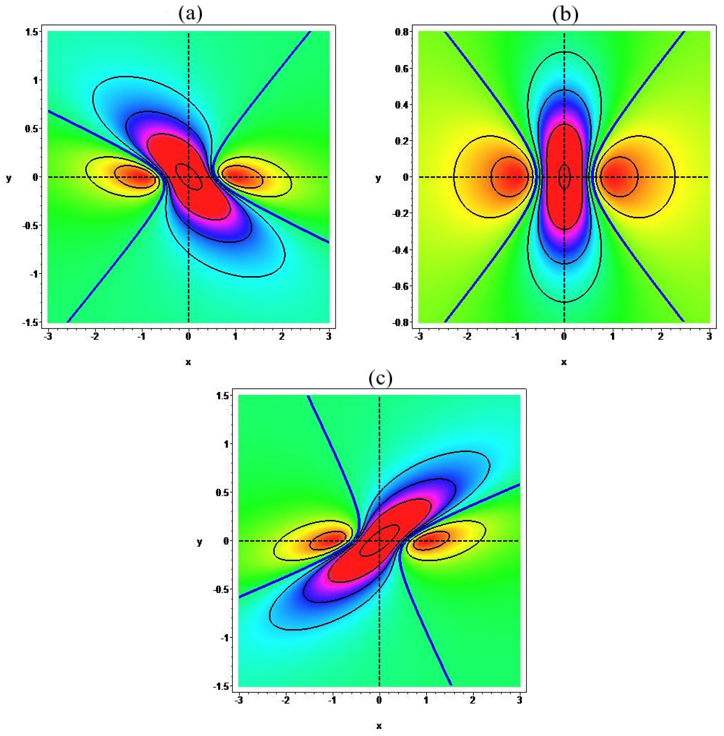
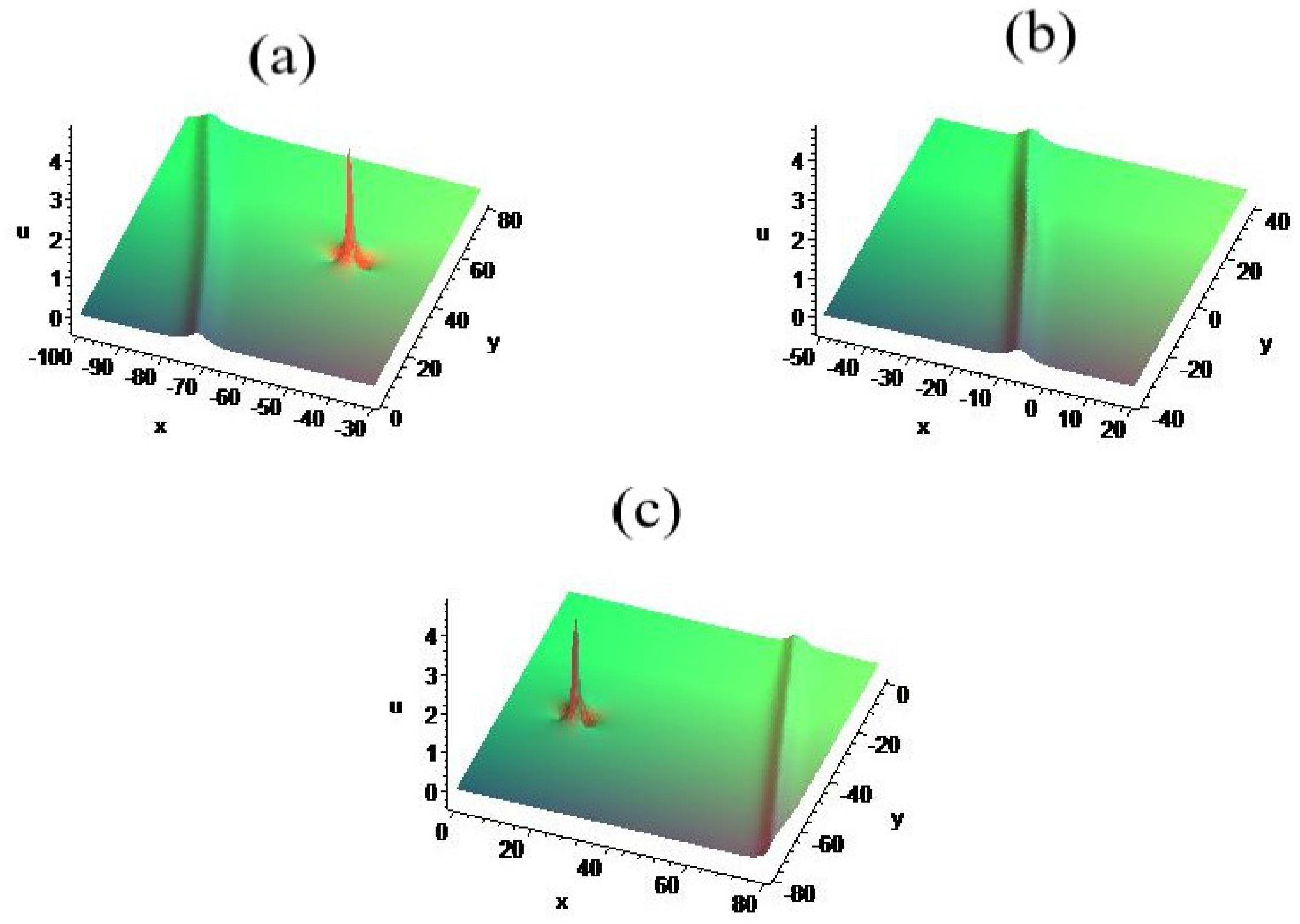
where and signify the horizontal and vertical velocities for the rational localized wave, respectively. The signs of determine the direction of propagation along the y-axis. In addition, the condition suggests that the rational localized wave (24) cannot be converted into a line localized wave [16]. What is more, it is easy to see from the straight line (27) that the inclined direction of the propagation trajectory to the x-axis is determined by the signs of : if , then , and the propagation trajectory passes through the first and the third quadrant in the -plane; if , then , and the propagation trajectory passes through the second and the forth quadrant in the -plane; if , then and , and the propagation trajectory is the y-axis. However, the symmetries of the rational localized wave are determined by the signs of : if , the rational localized wave leans to the right in the -plane; if , the rational localized wave is an axisymmetric graphic; if , the rational localized wave leans to the left in the -plane. Figure 1 illustrates three examples of the rational localized wave, and one of them represents a symmetrical rational localized wave with (Figure 1b), and another two are the skew rational localized wave figures with (Figure 1a,c). In Figure 1a, the rational localized wave leans to the left in the -plane. In Figure 1c, the rational localized wave leans to the right in the -plane. Therefore, according to the relations between and , we can come to the following conclusions:
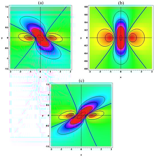
Figure 1.
Contour plots of the rational localized wave: (a) ; (b) ; (c) .
- (1)
- When , the solution (24) displays the oblique propagation of the skew rational localized wave. The rational localized wave leans to the right in the -plane, and its propagation trajectory passes through the first and the third quadrant. However, in this case, the direction of motion for the skew rational localized wave is completely determined by the signs of : if , then , and the skew rational localized wave moves up along the straight line (29) in the -plane; otherwise, it obliquely propagates along the opposite direction.
- (2)
- When , then and , and the rational localized wave moves along the y-axis and is asymmetric about the coordinate axis. Moreover, if , then , and the skew rational localized wave moves up along the y-axis; otherwise, it moves down along the y-axis.
- (3)
- When , the solution (24) also displays the oblique propagation of the skew rational localized wave. However, since , the propagation trajectory passes through the second and the forth quadrant in the -plane. The rational localized wave leans to the right, and the direction of motion is completely determined by the signs of : if , then , and the skew rational localized wave obliquely moves up along the straight line (29) in the -plane; otherwise, it obliquely propagates along the opposite direction.
- (4)
- When , the solution (24) displays the oblique propagation of the symmetrical rational localized wave, and its propagation trajectory passes through the second and the forth quadrant. Moreover, if , the symmetrical rational localized wave obliquely moves up along the straight line (29) in the -plane; otherwise, it obliquely propagates along the opposite direction.
- (5)
- When , the solution (24) displays the oblique propagation of the skew rational localized wave, and its propagation trajectory passes through the second and the forth quadrant in the -plane. However, the rational localized wave leans to the left in the -plane.
3. Interaction of a Rational Localized Wave and a Line Soliton
The interactions of nonlinear waves may demonstrate many interesting and novel dynamical features, and some of the phenomena have important physical meaning. In this section, we investigate the interactions of a rational localized wave and a line soliton. Through the analysis of the delay effect caused by the phase shift, we will show two different types of interaction between a rational localized wave and a line soliton: one is an absorb-emit interaction, and the other one is an emit-absorb interaction.
In order to illustrate the interaction behaviors between two kinds of localized waves, we consider the following interaction test function:
where:
and are complex numbers and real numbers. The solution determined by the interaction test function (31) with (32) contains two kinds of localized waves: one is a rational localized wave, and the other one is a line soliton. This implies the interactions between two kinds of localized waves. The functions and determine the rational localized wave before or after interaction, respectively. The parameters satisfy the relations (19) and (20). is a phase shift parameter to be determined later. The line soliton is determined by , and through (7) and (9), one can derive the exact expression of the line soliton:
where and the wave vector and the frequency s satisfy the following relation:
The solution (33) is localized along the straight line in the -plane, and the velocity is given by:
Further, substituting (31) with (32) into the extended bilinear form (10), we obtain the following result.
Theorem 2.
The extended bilinear form (10) has the solution (31), where the parameters satisfy the relations (19), (20), and (34), and the phase shift parameter is given by:
where . Further, combining with (7), (9), and (31)–(34), we can derive the interaction solution of a rational localized wave and a line soliton in the (2 + 1)-dimensional HSI equation. In particular, if , then the interaction solution degenerates to the rational localized wave solution.
Now, we consider the dynamical behaviors of the interaction solution determined by (31). For convenience in the following discussion, we assume that and that the parameters satisfy then one can obtain , and . With the above conditions and results, we can derive that the rational localized wave is symmetrical about the coordinate axes and obliquely moves down along the direction (30) in the -plane. The line soliton moves up along the direction (35) in the -plane. Therefore, under the above assumption, the interaction solution determined by (31) describes that a fast line soliton with speed overtakes a slow rational localized wave with speed .
To display the interaction process between two kinds of localized waves in detail, we firstly discuss the asymptotic form of the interaction solution as . Based on (21)–(23), the functions , and can be rewritten respectively as the following form:
where:
the parameters denote the real part and imaginary part of the complex parameter , respectively. The condition (20) implies . The velocities and are given by (30) and (35), respectively. To proceed, if , then we can derive the asymptotic expressions as :
and:
Thus, away from the interaction region, the interaction solution can be expressed as a sum of two noninteracting localized waves:
where denotes the rational localized wave and is given by (24). The localized wave denotes the line soliton and is given by (33).
Similarly, if , one can obtain:
Figure 2 and Figure 3 display two different interactions between a rational localized wave and a line soliton. As can be seen from Figure 2, when , the interaction solution determined by (31) describes the propagation of two separate localized waves; see Figure 2a. Interestingly, with the development of time, when two localized waves get close to each other, we observe that the slow rational localized wave gradually is absorbed by the right side of the fast line soliton. Two localized waves fuse to one line soliton; see Figure 2b. However, some time later, gradually, the slow rational localized wave is emitted from the left side of the fast line soliton; see Figure 2c. This interaction phenomenon can be referred to as an absorb-emit interaction phenomenon. Figure 3 is quite distinct from Figure 2. When , away from the interaction region, the interaction solution describes the propagation of two individual localized waves; see Figure 3a. More interestingly, with time evolution, when two localized waves come together, we find that a new rational localized wave gradually is emitted from the left side of the fast line soliton. Three localized waves are displayed; see Figure 3b. However, some time later, gradually, the original rational localized wave is absorbed by the right side of the line soliton; see Figure 3c. This interaction phenomenon can be referred to as an emit-absorb interaction phenomenon. These interactions are completely different from the completely non-elastic interaction between a rational localized wave and a line soliton in References [17,18].
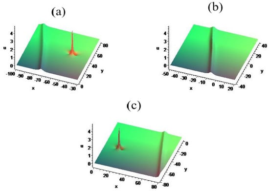
Figure 2.
Absorb-emit interaction with . The parameters are selected with , : (a) ; (b) ; (c) .
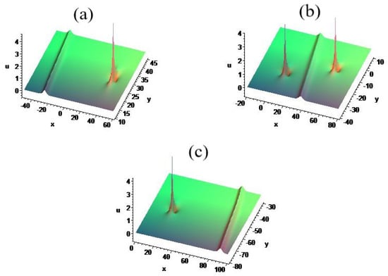
Figure 3.
Emit-absorb interaction with . The parameters are selected with , : (a) ; (b) ; (c) .
The above analysis shows two different interactions between a rational localized wave and a line soliton through numerical simulation. Now, we further explore the causes of two interaction phenomena through the theory analysis. Based on the above discussion, if , we can easily derive the following distance formulas from the rational localized wave to the line soliton before and after interaction in the -plane:
where the phase shift parameters and are given by (38). Therefore, we can obtain two critical points in time:
where and denote the encountering and parting time of two localized waves, respectively. Hence, it easy to see that the phase shift leads to the time delay between the encountering and parting time. Therefore, according to the relationship between and , we can easily draw the conclusion: if , when two localized waves meet, they do not move quickly away from each other. The phase shift leads to a delay in separating time, and the interaction will display the absorb-emit interaction phenomenon; see Figure 2. During this time , two localized waves fuse to one line soliton; see Figure 2b. If , when two localized waves come close to each other, the phase shift leads to a delay in encountering time, and the interaction will display the emit-absorb interaction phenomenon; see Figure 3. During this time , two rational localized waves and a line soliton coexist; see Figure 3b. In the process of interaction, it seems to generate one new line soliton. Indeed, this line soliton is not a new line soliton, but rather the original line soliton (33). If the total mass of the localized wave is defined by then we can obtain the following relations:
and:
where denotes the rational localized wave (24) and represents the line soliton (33). Equation (46) suggests that the interaction between two localized waves satisfies the mass conservation law. Therefore, the line soliton generated by the interaction between two localized waves is the original line soliton. The absorb or emit phenomenon of the line soliton cannot change the dynamical properties of the original line soliton.
In a word, assume that and denote the encountering and separating time of two localized waves, respectively. Then, the interactions between a rational localized wave and a line soliton can be classified into two categories:
- (1)
- When , the phase shift leads to a delay in separating time, and the interaction will display the absorb-emit interaction phenomenon. During this time , we can see that two localized waves fuse to one line soliton.
- (2)
- When , the phase shift leads to a delay in encountering time, and the interaction will display the emit-absorb interaction phenomenon. During this time , two rational localized waves and a line soliton coexist.
Furthermore, by controlling the time delay between the encountering and parting time of two localized waves, one can control the interaction time of two kinds of interaction phenomena.
4. Conclusions
In this work, we investigated the (2 + 1)-dimensional HSI equation with the translation parameter . Based on the extended Hirota bilinear form and the Hermitian quadratic form, we derived the rational localized wave solutions and further discussed their dynamical behaviors. It is shown that the oblique and skew characters of rational localized wave motion depend on the parameters and . When , the rational localized wave moves along the y-axis and is asymmetric about the coordinate axis. Otherwise, the skew rational localized wave moves obliquely with respect to the x-axis. When , the rational localized wave is symmetric about the coordinate axis. Otherwise, the rational localized wave is asymmetric about the coordinate axis. Finally, through theoretic analysis and numerical simulation, we mainly investigated and displayed the interactions between a rational localized wave and a line soliton. According to the time delay effect between the encountering and parting time of two localized waves, the interactions can be classified into two types: one is an absorb-emit interaction, and the other one is an emit-absorb interaction. Compared with the previous literature on the (2 + 1)-dimensional HSI equation, the obtained results with the parameter have richer dynamical behaviors. The oblique and skew characters of rational localized wave motion depend closely on the perturbation parameter . Furthermore, two different types of interaction between a rational localized wave and a line soliton were discussed in detail and illustrated graphically. These obtained localized wave solutions may provide some valuable information for understanding the relevant nonlinear wave phenomena. Following these ideas in this work, further study may be needed to see whether the (2 + 1)-dimensional HSI equation has another type of general high-order localized waves.
Author Contributions
Conceptualization, C.W.; Formal analysis, Y.Z., C.W. and X.Z.; Funding acquisition, C.W.; Investigation, Y.Z. and C.W.; Methodology, Y.Z., C.W. and X.Z.; Supervision, Y.Z. and C.W.; Writing—original draft, Y.Z. and C.W.; Writing—review—editing, Y.Z., C.W. and X.Z. All authors have read and agreed to the published version of the manuscript.
Funding
This research is supported by the National Natural Science Foundation of China (No. 11801240) and the Fund for Fostering Talents in Kunming University of Science and Technology (No. KKSY201707021).
Acknowledgments
The authors would like to express their sincere thanks to the Editors and Referees for their enthusiastic guidance and help.
Conflicts of Interest
The authors declare that there are no conflicts of interest regarding the publication of this paper.
References
- Hirota, R. The Direct Method in Soliton Theory; Cambridge University Press: New York, NY, USA, 2004. [Google Scholar]
- Zhang, Y.; Deng, S.F.; Chen, D.Y. The novel multi-soliton solutions of equation for shallow water waves. J. Phys. Soc. Jpn. 2003, 72, 763–764. [Google Scholar] [CrossRef]
- Lü, X.; Tian, B.; Sun, K.; Wang, P. Bell-polynomial manipulations on the Bäcklund transformations and Lax pairs for some soliton equations with one Tau-function. J. Math. Phys. 2010, 51, 113506. [Google Scholar] [CrossRef]
- Lü, X.; Ma, W.X.; Chen, S.T.; Khalique, C.M. A note on rational solutions to a Hirota–Satsuma-like equation. Appl. Math. Lett. 2016, 58, 13–18. [Google Scholar] [CrossRef]
- Wu, Y.Q. Asymptotic Behavior of Periodic Wave Solution to the Hirota–Satsuma Equation. Chin. Phys. Lett. 2011, 28, 060204. [Google Scholar] [CrossRef]
- Zhao, Z.L.; Zhang, Y.F. Periodic wave solutions and asymptotic analysis of the Hirota–Satsuma shallow water wave equation. Math. Meth. Appl. Sci. 2015, 38, 4262–4271. [Google Scholar] [CrossRef]
- Zhou, Y.; Manukure, S. Complexiton solutions to the Hirota–Satsuma–Ito equation. Math. Meth. Appl. Sci. 2019, 42, 2344–2351. [Google Scholar] [CrossRef]
- Ma, W.X. Interaction solutions to Hirota–Satsuma–Ito equation in (2 + 1)-dimensions. Front Math. Chin. 2019, 14, 619–629. [Google Scholar] [CrossRef]
- Zhou, Y.; Manukure, S.; Ma, W.X. Lump and lump-soliton solutions to the Hirota–Satsuma–Ito equation. Commun. Nonlinear. Sci. Numer. Simulat. 2019, 68, 56–62. [Google Scholar] [CrossRef]
- Liu, Y.Q.; Wen, X.Y.; Wang, D.S. The N-soliton solution and localized wave interaction solutions of the (2 + 1)-dimensional generalized Hirota–Satsuma–Ito equation. Comput. Math. Appl. 2019, 77, 947–966. [Google Scholar] [CrossRef]
- Liu, W.; Wazwaz, A.M.; Zheng, X.X. High-order breathers, lumps, and semi-rational solutions to the (2 + 1)-dimensional Hirota–Satsuma–Ito equation. Phys. Scr. 2019, 94, 075203. [Google Scholar] [CrossRef]
- Liu, J.G.; Zhu, W.H.; Zhou, L. Multi-wave, breather wave, and interaction solutions of the Hirota–Satsuma–Ito equation. Eur. Phys. J. Plus 2020, 135, 1–10. [Google Scholar] [CrossRef]
- Chen, S.J.; Ma, W.X.; Lü, X. Bäcklund transformation, exact solutions and interaction behavior of the (3 + 1)-dimensional Hirota–Satsuma–Ito-like equation. Commun. Nonlinear. Sci. Numer. Simulat. 2020, 83, 105135. [Google Scholar] [CrossRef]
- Wazwaz, A.M. Multiple-soliton solutions for the generalized (1 + 1)-dimensional and the generalized (2 + 1)-dimensional Ito equations. Appl. Math. Comput. 2008, 202, 840–849. [Google Scholar] [CrossRef]
- Horn, R.A.; Johnson, C.R. Matrix Analysis; Cambridge University Press: New York, NY, USA, 1990. [Google Scholar]
- Wang, C.J.; Fang, H.; Tang, X. State transition of lump-type waves for the (2 + 1)-dimensional generalized KdV equation. Nonlinear Dyn. 2019, 95, 2943–2961. [Google Scholar] [CrossRef]
- Wang, C.J.; Dai, Z.D.; Liu, C.F. Interaction between kink solitary wave and rogue wave for (2 + 1)-dimensional Burgers equation. Mediterr. J. Math. 2016, 13, 1087–1098. [Google Scholar] [CrossRef]
- Wang, C.J.; Fang, H. General high-order localized waves to the Bogoyavlenskii-Kadomtsev-Petviashvili equation. Nonlinear Dyn. 2020, 100, 583–599. [Google Scholar] [CrossRef]

Publisher’s Note: MDPI stays neutral with regard to jurisdictional claims in published maps and institutional affiliations. |
© 2020 by the authors. Licensee MDPI, Basel, Switzerland. This article is an open access article distributed under the terms and conditions of the Creative Commons Attribution (CC BY) license (http://creativecommons.org/licenses/by/4.0/).