An Accurate Approximation of the Two-Phase Stefan Problem with Coefficient Smoothing

Abstract

In this work, we consider the heat transfer problems with phase change. The mathematical model is described through a two-phase Stefan problem and defined in the whole domain that contains frozen and thawed subdomains. For the numerical solution of the problem, we present three schemes based on different smoothing of the sharp phase change interface. We propose the method using smooth coefficient approximation based on the analytical smoothing of discontinuous coefficients through an error function with a given smoothing interval. The second method is based on smoothing in one spatial interval (cell) and provides a minimal length of smoothing calculated automatically for the given values of temperatures on the mesh. The third scheme is a convenient scheme using a linear approximation of the coefficient on the smoothing interval. The results of the numerical computations on a model problem with an exact solution are presented for the one-dimensional formulation. The extension of the method is presented for the solution of the two-dimensional problem with numerical results.

1. Introduction

One of the urgent problems of mathematical physics is the Stefan problem, which describes heat transfer with a phase change of matter. An example of physical processes with phase transitions is the problem of melting ice with a movable boundary between water and ice, the problem of melting a solid with an unknown boundary between the solid and liquid phases, and the heat transfer processes in permafrost areas. The Stefan problem is an initial-boundary value problem of a parabolic differential equation with discontinuous coefficients on the phase change interfaces. The phase change occurs for a given value of temperature (freezing point), where the energy balance on the interface is written in the form of the Stefan condition and represented as a sharp interface (a moving-boundary problem).

In the numerical solution of the Stefan problem, a major difficulty is associated with the tracking of the phase change interface evolution. The enthalpy method was presented in [1,2,3,4], where the concept of effective heat capacity was introduced through various methods of smoothing of discontinuous coefficients. The general approach of thermodynamic functions was presented in [5], where an online application was implemented to generate the first-order derivatives of the thermodynamic parameters for a closed system. The substantiation of the correctness and numerical methods for solving various topical applied problems of the Stefan type were summarized in the review paper [6] and the monographs [7,8,9]. The relaxed linearization methods for the solution of the heat transfer problem using finite element approximation were presented in [4]. An efficient enthalpy-based numerical approach with a trust region minimization algorithm was introduced in [10] with various smoothing functions. In [11], the mathematical model with the separate evolution of the phase change interface from the heat equation was presented with XFEMapproximation.

In this work, we consider an enthalpy method with different types of smoothing functions. We propose a smooth coefficient approximation-based on the analytical smoothing of discontinuous coefficients using the error function with a given smoothing interval. We study a grid and time step convergence to examine the accuracy of the method for different lengths of smoothing intervals and compared to the regular linear smoothing. The novel method with smoothing in one spatial interval is proposed. The method provides a minimal length of smoothing that is calculated automatically for the given temperature values on the mesh. We start with the presentation of the methods for the one-dimensional formulation of the heat equation and perform convergence studies against the grid and time-step sizes, where we calculate the errors between analytical and numerical solutions using the proposed smoothing methods. Then, we generalize the methods for finite element approximations and present the results for two-dimensional model problems. Triangular elements are used, but the formulation can be extended for any type of element.

The paper is organized as follows. In Section 2, we describe the problem formulation. In Section 3, we consider the problem in the one-dimensional domain and present a finite difference approximation. In order to construct an approximation, we present three schemes with different smoothing of discontinuous coefficients, which reduces the Stefan problem to a quasilinear problem for a parabolic equation with smooth coefficients. The generalization of the presented schemes is given in Section 4, where we present the finite element approximation for one- and two-dimensional problems. Numerical results for the model problem are presented in Section 5 for one- and two-dimensional formulations, where we investigate the accuracy of the proposed schemes with different types of smoothing. For the one-dimensional problem, we compare the numerical results with the exact solution. A result of the two-dimensional problem is presented for two geometries. The paper ends with the Conclusion.

2. Stefan Problem

We consider the two-phase Stefan problem in the domain $\mathrm{\Omega }$. Let $u(x,t)$ be an unknown function (temperature) and $u^{*}$ be a phase change temperature that occurs on the phase change interface $\xi$:

$$\xi =\{x\in \mathrm{\Omega }, u(x,t)=u^{*}\},\hspace{1em}\mathrm{\Omega }={\mathrm{\Omega }}_1\cup {\mathrm{\Omega }}_2,\hspace{1em}{\mathrm{\Omega }}_1\cap {\mathrm{\Omega }}_2=\xi$$

where ${\mathrm{\Omega }}_1$ is a frozen zone and ${\mathrm{\Omega }}_2$ is a thawed zone:

$${\mathrm{\Omega }}_1(t)=\{x\in \mathrm{\Omega }, u(x,t)<u^{*}\},\hspace{1em}{\mathrm{\Omega }}_2(t)=\{x\in \mathrm{\Omega }, u(x,t)>u^{*}\}.$$

We have conductive heat transfer in ${\mathrm{\Omega }}_1$ and ${\mathrm{\Omega }}_2$:

$$\begin{array}{cc}\hfill \hspace{1em}& c_1\frac{\partial u_1}{\partial t}-\nabla ·\left(k_1\nabla u_1\right)=0,\hspace{1em}x\in {\mathrm{\Omega }}_1,\hspace{1em}t\in (0,T],\hfill \\ \hfill \hspace{1em}& c_2\frac{\partial u_2}{\partial t}-\nabla ·\left(k_2\nabla u_2\right)=0,\hspace{1em}x\in {\mathrm{\Omega }}_2,\hspace{1em}t\in (0,T].\hfill \end{array}$$

(1)

On the phase change interface $\xi$, we have a continuous temperature and the jump of the heat flux, which is associated with the latent heat of fusion for water [1,2]:

$$\begin{array}{cc}\hfill \hspace{1em}& u_1=u_2=u^{*},\hspace{1em}x\in \xi ,\hfill \\ \hfill \hspace{1em}& (k_1\nabla u_1-k_2\nabla u_2,\nabla \xi )=D\frac{d\xi }{dt},\hspace{1em}x\in \xi .\hfill \end{array}$$

(2)

We write the system of Equations (1) and (2) as the two-phase Stefan problem in domain $\mathrm{\Omega }$:

$$\left(c(u)+D\delta (u-u^{*})\right)\frac{\partial u}{\partial t}-\nabla ·\left(k(u)\nabla u\right)=0,\hspace{1em}x\in \mathrm{\Omega },\hspace{1em}t\in (0,T],$$

(3)

where $\delta$ is the Dirac delta function:

$$\delta (u-u^{*})=\frac{d\eta (u-u^{*})}{du},\hspace{1em}\eta (u-u^{*})=\left\{\begin{array}{cc}1,& u\ge u^{*},\\ 0,& u<u^{*},\end{array}\right.$$

and:

$$c(u)=\left\{\begin{array}{cc}{c}_1(u),& u<u^{*},\\ c_2(u),& u>u^{*},\end{array}\right.\hspace{1em}k(u)=\left\{\begin{array}{cc}{k}_1(u),& u<u^{*},\\ k_2(u),& u>q{u}^{*}.\end{array}\right.$$

The coefficients of the equation depend on the function $u(x,t)$ and have a discontinuity of the first kind at $u(x,t)=u^{*}$.

The main difficulty in the presented problem is associated with dynamic tracking of the phase change interface. Since the $\delta$ coefficient of Equation (3) at $u(x,t)=u^{*}$ becomes infinity, a numerical solution of this equation is possible after smoothing the function $\eta$ [1,2,10]. Let the phase change not occur instantaneously, but take place in a small temperature range (slushy zone). The discontinuous coefficients $\eta$ of Equation (3) are replaced by bounded continuous (smooth) functions of temperature $\tilde{\eta }(u)$:

$$\left(\tilde{c}(u)+D\tilde{\delta }(u-u^{*})\right)\frac{\partial u}{\partial t}-\nabla ·\left(\tilde{k}(u)\nabla u\right)=0,\hspace{1em}x\in \mathrm{\Omega },\hspace{1em}t\in (0,T],$$

(4)

where:

$$\tilde{c}(u)=c_1+\tilde{\eta }(u)(c_2-c_1),\hspace{1em}\tilde{k}(u)=k_1+\tilde{\eta }(u)(k_2-k_1),\hspace{1em}\tilde{\delta }=\frac{d\tilde{\eta }(u)}{du}.$$

The resulting Equation (4) is a quasilinear parabolic equation with positive, bounded, continuous (smooth) coefficients, which depends on the coefficient smoothing procedure.

We have the following initial condition:

$$u(x,0)=u_0(x),\hspace{1em}x\in \mathrm{\Omega },$$

(5)

and boundary conditions:

$$\begin{array}{cc}\hfill u=g(t),& \hspace{1em}x\in {\mathrm{\Gamma }}_1,\hspace{1em}t\in (0,T],\hfill \\ \hfill -\tilde{k}(u)\frac{\partial u}{\partial n}=0,& \hspace{1em}x\in {\mathrm{\Gamma }}_2,\hspace{1em}t\in (0,T],\hfill \end{array}$$

(6)

where ${\mathrm{\Gamma }}_1\cup {\mathrm{\Gamma }}_2=\partial \mathrm{\Omega }$.

Next, we present two novel approaches to the accurate approximation of the Stefan problem and consider a convenient approach with a linear approximation of the $\eta$ function. First, we define a smooth approximation of coefficients using the error function and linear approximation. Then, we present a novel approach with smoothing in one spatial interval that provides a very accurate approximation of the problem and does not depend on the interval of a slushy zone, which is hard to define because it depends on the speed of phase change interface propagation and can vary in space and time.

3. Approximation of the One-Dimensional Problem

Let $\mathrm{\Omega }$ be the one-dimensional computational domain ($\mathrm{\Omega }=[0,L]$) and ${\mathcal{T}}_h$ be the uniform mesh:

$${\mathcal{T}}_h=\{x_i=ih, i=0,1,\dots ,N; h=L/N\},$$

where h is the mesh size. For the time approximation, we use an implicit scheme with linearization from the previous time layer, where $t^m=m\tau$ for $m=0,1,\dots ,M$ and $\tau =T/M$ is the time step size.

We have the following finite difference approximation of the problem (4)–(6) with smooth coefficients on the grid ${\mathcal{T}}_h$:

$$\left({\tilde{c}}_i^{m-1}+D{\tilde{\delta }}_i^{m-1}\right)\frac{u_i^m-u_i^{m-1}}{\tau } h+q_{i+0.5}^m-q_{i-0.5}^m=0,\hspace{1em}m=1,2,\dots ,M,$$

(7)

where:

$$q_{i+0.5}^m=-{\tilde{k}}_{i+0.5}^{m-1}\frac{u_{i+1}^m-u_i^m}{h},$$

(8)

for $i=1,\dots ,N$.

We consider the approximation (7) with the following initial conditions:

$$u_i^0=u_0(x_i),\hspace{1em}i=0,\dots ,N.$$

(9)

Let ${\mathrm{\Gamma }}_1$ and ${\mathrm{\Gamma }}_2$ be the left and right boundaries, $x=0$ and $x=L$. For the Dirichlet boundary condition on $x=0$, we have:

$$\begin{array}{c}\hfill u_i^m=g(t^m),\hspace{1em}i=0.\end{array}$$

(10)

For the Neumann boundary condition on $x=L$, we have:

$$\begin{array}{c}\hfill q_{i+0.5}^m=0,\hspace{1em}i=N,\end{array}$$

(11)

for $m=1,2,\dots ,M$.

3.1. Smoothing on the $\Delta$ Interval

Let $[u^{*}-\Delta ,u^{*}+\Delta ]$ be the smoothing interval (slushy zone). For the coefficients of Equations (7) and (8), we have:

$$\begin{array}{cc}\hfill \hspace{1em}& {\tilde{k}}_{i+0.5}^m=\frac{2}{{({\tilde{k}}_{i+1}^m)}^{-1}+{({\tilde{k}}_i^m)}^{-1}},\hspace{1em}{\tilde{k}}_i^m=k_1+{\tilde{\eta }}_i^m(k_2-k_1),\hfill \\ \hfill \hspace{1em}& {\tilde{c}}_i^m=c_1+{\tilde{\eta }}_i^m(c_2-c_1),\hspace{1em}{\tilde{\delta }}_i^m=\frac{d{\tilde{\eta }}_i^m}{d{u}_i^m}.\hfill \end{array}$$

(12)

Note that, in this approximation, coefficients ${\tilde{c}}_i^m$, ${\tilde{k}}_i^m$ are defined on the mesh nodes, and ${\tilde{k}}_{i+0.5}^m$ is defined on the cell as the harmonic average of the values on nodes $x_{i+1}$ and $x_i$.

In schemes with smoothing on the $\Delta$ interval, the coefficients $\tilde{\eta }$ and $\tilde{\delta }$ are defined in each node of the mesh and calculated using the given value of function $u_i$ on current node $x_i$:

$${\tilde{\eta }}_i^m=\tilde{\eta }(u_i^m),\hspace{1em}{\tilde{\delta }}_i^m=\tilde{\delta }(u_i^m).$$

We consider the following smoothing of discontinuous coefficients and define smooth functions $\tilde{\eta }$ as follows:

• Smoothing on the $\Delta$ interval using the error function:

  $$\tilde{\eta }(u)=\frac{1}{2}\left(1+\mathrm{erf}\left(\frac{u-u^{*}}{\sqrt{2}\Delta }\right)\right),\hspace{1em}\tilde{\delta }(u)=\frac{1}{\sqrt{2\pi }\Delta }exp\left(-\frac{{(u-u^{*})}^2}{2{\Delta }^2}\right).$$

  (13)
• Linear smoothing in the $\Delta$ interval:

  $$\tilde{\eta }(u)=\left\{\begin{array}{cc}1,& u\ge u^{*}+\Delta ,\\ \frac{(u-u^{*}+\Delta )}{2\Delta },\hspace{1em}& u^{*}-\Delta <u<u^{*}+\Delta ,\\ 0,& u\le u^{*}-\Delta ,\end{array}\right.\hspace{1em}\tilde{\delta }(u)=\left\{\begin{array}{cc}0,& u\ge u^{*}+\Delta ,\\ \frac{1}{2\Delta },& u^{*}-\Delta <u<u^{*}+\Delta ,\\ 0,& u\le u^{*}-\Delta .\end{array}\right.$$

  (14)

We note that the accuracy of the presented schemes depends on the choice of the $\Delta$ parameter. If we choose a very large $\Delta$ interval, we overestimate the slushy zone interval and obtain large errors. In general, the parameter $\Delta$ should depend on the spatial and time meshes in approximation as the parameter highly depends on the speed of the freezing front propagation. Other methods of such procedures were proposed in [10], where exponential- or sinusoidal-based functions can be used to smooth function $\tilde{\eta }$ on the $\Delta$ interval. In [1,2], the authors presented smoothing using polynomials of a given degree.

3.2. Smoothing in One Spatial Interval

In order to construct a scheme without the estimation of the smoothing interval parameter $\Delta$, we present a novel method to an accurate approximation of the two-phase Stefan problem by choosing the minimal possible interval of the slushy zone for the current mesh.

Let a phase change occur on one spatial interval $[x_i,x_{i+1}]$ if $(u_i-u^{*})·(u_{i+1}-u^{*})<0$. In this scheme, $\tilde{\eta }$ and $\tilde{\delta }$ are defined on cell $[x_i,x_{i+1}]$ and approximated using values of the functions $u_i$ and $u_{i+1}$. For the coefficients of Equations (7) and (8), we have:

$${\tilde{k}}_{i+0.5}^m=k_1+{\tilde{\eta }}_{i+0.5}^m(k_2-k_1),\hspace{1em}{\tilde{c}}_i^m=\left\{\begin{array}{cc}{c}_1,\hfill & \hspace{1em}{u}_i^m<u^{*},\hfill \\ c_2,\hfill & \hspace{1em}{u}_i^m\ge u^{*},\hfill \end{array}\right.,\hspace{1em}{\tilde{\delta }}_i^m={\tilde{\delta }}_{i-0.5}^m+{\tilde{\delta }}_{i+0.5}^m,$$

(15)

where coefficient ${\tilde{c}}_i^m$ is defined on each node $x_i$ and coefficients ${\tilde{\eta }}_{i+0.5}^m$ and ${\tilde{\delta }}_{i+0.5}^m$ are calculated taking into account the presence or absence of the phase change interface in the temperature interval $[u_i,u_{i+1}]$.

For the accurate approximation of the two-phase Stefan problem, we present a smoothing in one spatial interval:

$${\tilde{\eta }}_{i+0.5}=\left\{\begin{array}{cc}1,\hfill & \hspace{1em}{u}_i\ge u^{*} \mathrm{and} u_{i+1}\ge u^{*},\hfill \\ (u_{i+1}-u^{*})/(u_{i+1}-u_i),\hfill & \hspace{1em}{u}_i<u^{*} \mathrm{and} u_{i+1}>u^{*},\hfill \\ (u_i-u^{*})/(u_i-u_{i+1}),\hspace{1em}\hfill & \hspace{1em}{u}_i>u^{*} \mathrm{and} u_{i+1}<u^{*},\hfill \\ 0,\hfill & \hspace{1em}{u}_i<u^{*} \mathrm{and} u_{i+1}<u^{*},\hfill \end{array}\right.,$$

(16)

$${\tilde{\delta }}_{i+0.5}=\left\{\begin{array}{cc}0,\hfill & \hspace{1em}{u}_i\ge u^{*} \mathrm{and} u_{i+1}\ge u^{*},\hfill \\ (u_{i+1}-u^{*})/{(u_{i+1}-u_i)}^2,\hfill & \hspace{1em}{u}_i<u^{*} \mathrm{and} u_{i+1}>u^{*},\hfill \\ -(u_{i+1}-u^{*})/{(u_i-u_{i+1})}^2,\hspace{1em}\hfill & \hspace{1em}{u}_i>u^{*} \mathrm{and} u_{i+1}<u^{*},\hfill \\ 0,\hfill & \hspace{1em}{u}_i<u^{*} \mathrm{and} u_{i+1}<u^{*}.\hfill \end{array}\right.$$

(17)

At the calculation of the phase change interface position, we use a linear interpolation of the desired function within the indicated temperature interval. Further, we determine the value of the corresponding coefficient for the difference equation.

4. Generalization of Methods for Finite Element Approximation

In this section, we generalize the presented algorithm for the solution of the two-dimensional problems on unstructured meshes [12]. We use a finite element method and set:

$$V=\{v\in H(\mathrm{\Omega }): v=g_1 \mathrm{on} {\mathrm{\Gamma }}_1\},\hspace{1em}{V}^{\prime }=\{v\in H(\mathrm{\Omega }): v=0 \mathrm{on} {\mathrm{\Gamma }}_1\}.$$

For the heat problem (4)–(6), we have the following variational formulation of the problem: find $u^m\in V$ such that:

$$s(u^m-u^{m-1},v)+a(u^m,v)=0,\hspace{1em}\forall v\in V^{\prime },$$

(18)

where:

$$s(u^m,v)=\frac{1}{\tau }{\int }_{\mathrm{\Omega }}\left({\tilde{c}}^{m-1}+D{\tilde{\delta }}^{m-1}\right)u^m v dx,\hspace{1em}a(u^m,v)={\int }_{\mathrm{\Omega }}{\tilde{k}}^{m-1}\nabla u^m·\nabla v dx.$$

Let ${\mathcal{T}}_h$ be the mesh for the domain $\mathrm{\Omega }$:

$${\mathcal{T}}_h={\cup }_i{K}_i,\hspace{1em}i=1,\dots N_c,$$

where $N_c$ is the number of grid cells.

We replace the space V by a finite dimensional subspace $V_h$, $V_h\subset V$. We suppose that space $V_h$ is composed of piecewise linear basis functions ${\varphi }_i$ on the grid cell, $i=1,\dots N$ and $N=\dim (V_h)$ is the number of nodes (vertices) for linear basis functions. We have the following decomposition of $u_h$ in the basis of $V_h$:

$$u_h(x,t^m)=\sum _{j=1}^N{u}_j^m{\varphi }_j(x).$$

Problem (18) is replaced by the following discrete problem:

$$\sum _{j=1}^N{u}_j^m\left(s({\varphi }_j,{\varphi }_i)+a({\varphi }_j,{\varphi }_i)\right)=l({\varphi }_i),\hspace{1em}i=1,\dots N,$$

where $l({\varphi }_i)=s(u_h^{m-1},{\varphi }_i)$

We have the following discrete system in the matrix form for $U={(u_1,\dots ,u_N)}^T$:

$$(S^{m-1}+A^{m-1})U^m=F^{m-1},$$

where $S^m$ and $A^m$ are global mass and stiffness matrices:

$$S^m=\sum _{i=1}^{N_c}{S}^{m,i},\hspace{1em}{A}^m=\sum _{i=1}^{N_c}{A}^{m,i},\hspace{1em}{F}^m=S^m{U}^m.$$

Here, $S^{m,i}$ and $A^{m,i}$ are local matrices in cell $K_i$:

$$A^{m,i}=\{A_{lj}^{K_i}\},\hspace{1em}{A}_{lj}^{K_i}=a^{K_i}({\varphi }_l,{\varphi }_j)={\int }_{K_i}{\tilde{k}}^{m-1}\nabla {\varphi }_l·\nabla {\varphi }_j dx,$$

$$S^{m,i}=\{S_{lj}^{K_i}\},\hspace{1em}{S}_{lj}^{K_i}=s^{K_i}({\varphi }_l,{\varphi }_j)={\int }_{K_i}\left({\tilde{c}}^{m-1}+D{\tilde{\delta }}^{m-1}\right){\varphi }_l {\varphi }_j dx,$$

where:

$$\tilde{c}(u)=c_1+\tilde{\eta }(u)(c_2-c_1),\hspace{1em}\tilde{k}(u)=k_1+\tilde{\eta }(u)(k_2-k_1),\hspace{1em}\tilde{\delta }=\frac{d\tilde{\eta }(u)}{du}.$$

In order to obtain a similar form of discrete system as in the previous section with finite difference approximation, we suppose that coefficient ${\tilde{k}}_i$ is defined in each cell ($i=1,\dots ,N_c$) and coefficient ${\tilde{c}}_j$ is defined on mesh node ($j=1,\dots ,N$). We use a trapezoidal integration to obtain a diagonal mass matrix.

4.1. Smoothing on the $\Delta$ Interval

Similarly to the previous section, $\tilde{\eta }$ and $\tilde{\delta }$ are defined in each node of the mesh and calculated using the given value of function $u_i$ on current node $x_i$:

$${\tilde{\eta }}_i^m=\tilde{\eta }(u_i^m),\hspace{1em}{\tilde{\delta }}_i^m=\tilde{\delta }(u_i^m),$$

with the following approximations:

• Smoothing on the $\Delta$ interval using the error function:

  $$\tilde{\eta }(u)=\frac{1}{2}\left(1+\mathrm{erf}\left(\frac{u-u^{*}}{\sqrt{2}\Delta }\right)\right),\hspace{1em}\tilde{\delta }(u)=\frac{1}{\sqrt{2\pi }\Delta }exp\left(-\frac{{(u-u^{*})}^2}{2{\Delta }^2}\right).$$

  (19)
• Linear smoothing on the $\Delta$ interval:

  $$\tilde{\eta }(u)=\left\{\begin{array}{cc}1,& u\ge u^{*}+\Delta ,\\ \frac{(u-u^{*}+\Delta )}{2\Delta },\hspace{1em}& u^{*}-\Delta <u<u^{*}+\Delta ,\\ 0,& u\le u^{*}-\Delta ,\end{array}\right.\hspace{1em}\tilde{\delta }(u)=\left\{\begin{array}{cc}0,& u\ge u^{*}+\Delta ,\\ \frac{1}{2\Delta },& u^{*}-\Delta <u<u^{*}+\Delta ,\\ 0,& u\le u^{*}-\Delta .\end{array}\right.$$

  (20)

Let $n_K$ be the number of vertices in cell K, where $n_K=2$ for the one-dimensional problem and $n_K=3$ for the two-dimensional problem with triangular cells. For the stiffness matrix, we have:

$$A_{lj}^{K_i}={\tilde{k}}_{K_i}^{m-1}{\int }_{K_i}\nabla {\varphi }_l·\nabla {\varphi }_j dx,$$

where:

$${\tilde{k}}_{K_i}^m=\frac{n_K}{{\sum }_{j=1}^{n_K}{({\tilde{k}}_j^m)}^{-1}},\hspace{1em}{\tilde{k}}_j^m=k_1+{\tilde{\eta }}_j^m(k_2-k_1).$$

For the mass matrix with trapezoidal integration, we have:

$$S_{jj}^{K_i}=\frac{|K_i|}{n_K}\left({\tilde{c}}_j^{m-1}+D{\tilde{\delta }}_j^{m-1}\right),\hspace{1em}{S}_{lj}^{K_i}=0,\hspace{1em} \mathrm{for} l\ne j,$$

where:

$${\tilde{c}}_j^m=c_1+{\tilde{\eta }}_j^m(c_2-c_1).$$

Here, coefficients ${\tilde{c}}_j^m$, ${\tilde{k}}_j^m$ are defined on the mesh nodes, and ${\tilde{k}}_{K_i}^m$ is defined on the cell as the harmonic average of the values on the cell nodes.

4.2. Smoothing in One Mesh Cell

Similar to smoothing in one spatial interval for the one-dimensional problem, we construct smoothing in one cell of the grid for the general case, where a cell can be of any shape (interval, triangle, tetrahedron, quadrilateral, etc.).

Let a phase change occur on one mesh cell $K_i$ if $(u_i-u^{*})·(u_j-u^{*})<0$ for $i,j=1,\dots ,n_K$ ($n_K$ is the number of vertices of mesh cell). We define $\tilde{\eta }$ and $\tilde{\delta }$ on cell $K_i$ using a similar approximation by the values of the function $u_j^{K_i}$ in cell $K_i$ ($j=1,\dots ,n_K$). For the stiffness matrix, we have:

$$A_{lj}^{K_i}={\tilde{k}}_{K_i}^{m-1}{\int }_{K_i}\nabla {\varphi }_l·\nabla {\varphi }_j dx$$

with:

$${\tilde{k}}_{K_i}^m=k_1+{\tilde{\eta }}_{K_i}^m(k_2-k_1),$$

(21)

For the mass matrix, we have:

$$S_{jj}^{K_i}=\frac{|K_i|}{n_K} {\tilde{c}}_j^{m-1}+\left|K_i\right| D {\tilde{\delta }}_{K_i,j}^{m-1},\hspace{1em}{S}_{lj}^{K_i}=0,\hspace{1em} \mathrm{for} l\ne j,$$

with:

$${\tilde{c}}_j^m=\left\{\begin{array}{cc}{c}_1,\hfill & \hspace{1em}{u}_j^{K_i,m}<u^{*},\hfill \\ c_2,\hfill & \hspace{1em}{u}_j^{K_i,m}\ge u^{*},\hfill \end{array}\right.\hspace{1em}{\tilde{\delta }}_{K_i,j}^m=\frac{d{\tilde{\eta }}_{K_i}^m}{d{u}_j^{K_i,m}}.$$

(22)

where $u_j^{K_i,m}$ is the value of function u on node j in cell $K_i$ and $j,l=1,\dots ,n_v$. Here, ${\tilde{c}}_j^{K_i,m}$ is defined on mesh vertex j in cell $K_i$ using the corresponding value of function u, and ${\tilde{k}}_{K_i}^m$ is defined on cell $K_i$. The coefficient ${\tilde{\eta }}_{K_i}^m$ is calculated by taking into account the presence or absence of the phase change interface in cell $K_i$.

For the one-dimensional problem with $n_K=2$, we have cell $K_i=[x_i,x_{i+1}]$ with $|K_i|=x_{i+1}-x_i=h$ and $u_i=u_1^{K_i}$, $u_{i+1}=u_2^{K_i}$. Therefore, we have:

$${\tilde{\eta }}_{K_i}=\left\{\begin{array}{cc}1,\hfill & \hspace{1em}{u}_1^{K_i}\ge u^{*} \mathrm{and} u_2^{K_i}\ge u^{*},\hfill \\ (u_2^{K_i}-u^{*})/(u_2^{K_i}-u_1^{K_i}),\hfill & \hspace{1em}{u}_1^{K_i}<u^{*} \mathrm{and} u_2^{K_i}>u^{*},\hfill \\ (u_1^{K_i}-u^{*})/(u_1^{K_i}-u_2^{K_i}),\hspace{1em}\hfill & \hspace{1em}{u}_1^{K_i}>u^{*} \mathrm{and} u_2^{K_i}<u^{*},\hfill \\ 0,\hfill & \hspace{1em}{u}_1^{K_i}<u^{*} \mathrm{and} u_2^{K_i}<u^{*},\hfill \end{array}\right.$$

(23)

$${\tilde{\delta }}_{K_i,1}=\left\{\begin{array}{cc}0,\hfill & \hspace{1em}{u}_1^{K_i}\ge u^{*} \mathrm{and} u_2^{K_i}\ge u^{*},\hfill \\ (u_2^{K_i}-u^{*})/{(u_2^{K_i}-u_1^{K_i})}^2,\hfill & \hspace{1em}{u}_1^{K_i}<u^{*} \mathrm{and} u_2^{K_i}>u^{*},\hfill \\ -(u_2^{K_i}-u^{*})/{(u_1^{K_i}-u_2^{K_i})}^2,\hspace{1em}\hfill & \hspace{1em}{u}_1^{K_i}>u^{*} \mathrm{and} u_2^{K_i}<u^{*},\hfill \\ 0,\hfill & \hspace{1em}{u}_1^{K_i}<u^{*} \mathrm{and} u_2^{K_i}<u^{*},\hfill \end{array}\right.$$

(24)

$${\tilde{\delta }}_{K_i,2}=\left\{\begin{array}{cc}0,\hfill & \hspace{1em}{u}_1^{K_i}\ge u^{*} \mathrm{and} u_2^{K_i}\ge u^{*},\hfill \\ -(u_1^{K_i}-u^{*})/{(u_2^{K_i}-u_1^{K_i})}^2,\hfill & \hspace{1em}{u}_1^{K_i}<u^{*} \mathrm{and} u_2^{K_i}>u^{*},\hfill \\ (u_1^{K_i}-u^{*})/{(u_1^{K_i}-u_2^{K_i})}^2,\hspace{1em}\hfill & \hspace{1em}{u}_1^{K_i}>u^{*} \mathrm{and} u_2^{K_i}<u^{*},\hfill \\ 0,\hfill & \hspace{1em}{u}_1^{K_i}<u^{*} \mathrm{and} u_2^{K_i}<u^{*}.\hfill \end{array}\right.$$

(25)

Note that this approximation is equal to the smoothing presented in the previous section for the one-dimensional formulation using the finite-difference method.

Before the generalization of the smoothing in one mesh cell, we present a brief explanation of the concept that we used in this method. Let $V_{+}^{K_i}$ and $V_{-}^{K_i}$ be the volume of thawed and frozen zones in cell $K_i$, $V^{K_i}=\left|K_i\right|$ the volume of the cell, and $V^{K_i}=V_{+}^{K_i}+V_{-}^{K_i}$. The coefficient $\eta$ is the unfrozen water concentration that can be represented as a fraction of the thawed zone from the cell volume:

$${\tilde{\eta }}_{K_i}=\frac{V_{+}^{K_i}}{V^{K_i}},$$

where $V_{+}^{K_i}=V^{K_i}$ for $u_j^{K_i}\ge u^{*}$, $\forall j=1,\dots ,n_v$ ($\tilde{\eta }=1$) and $V_{+}^{K_i}=0$ for $u_j^{K_i}<u^{*}$, $\forall j=1,\dots ,n_v$ ($\tilde{\eta }=0$). In order to calculate the volume of the thawed zone in mesh cell $V_{+}^{K_i}$, we use a linear approximation of the temperature in cell.

In the one-dimensional case, we have:

$$u(x)=u_1{\varphi }_1(x)+u_2{\varphi }_2(x),$$

where:

$${\varphi }_1(x)=\frac{x_1-x}{x_2-x_1},\hspace{1em}{\varphi }_2(x)=\frac{x-x_1}{x_2-x_1}.$$

Therefore, the location of the phase change interface in cell $K_i$ is the following (see Figure 1):

$$x^{*}=x_1+(x_2-x_1)\frac{u^{*}-u_1}{u_2-u_1},$$

and therefore, we obtain:

$${\tilde{\eta }}_{K_i}=\frac{x^{*}-x_1}{x_2-x_1}=\frac{u_1-u^{*}}{u_1-u_2}\hspace{1em} \mathrm{for} u_1>u_2,$$

$${\tilde{\eta }}_{K_i}=1-\frac{x^{*}-x_1}{x_2-x_1}=1-\frac{u^{*}-u_1}{u_2-u_1}=\frac{u_2-u^{*}}{u_2-u_1}\hspace{1em} \mathrm{for} u_2>u_1,$$

for the one-dimensional problem when the phase change occurs in cell $K_i$, $(u_i-u^{*})·(u_2-u^{*})<0$. In the approximation construction for the two-dimensional case, we use a similar approach, where we find an interface position on each edge between two nodes and use it to calculate a fraction of the unfrozen zone in cell $K_i$. For example, for the case with $u_1>u^{*}$, $u_2<u^{*}$, and $u_3<u^{*}$ (see Figure 1), we have:

$${\tilde{\eta }}_{K_i}=\frac{V_{+}^{K_i}}{V^{K_i}}=\left(\frac{u_1-u^{*}}{u_1-u_2}\right)\left(\frac{u_1-u^{*}}{u_1-u_3}\right),$$

where the unfrozen zone volume and the volume of the cell are calculated as the area of corresponding triangles. Approximations of the $\tilde{\eta }$ for other cases can be calculated in a similar way. In Figure 1, we present an illustration of thawed and frozen zones on mesh cell $K_i$.

Finally, for the two-dimensional formulation with triangular cells, we have:

$${\tilde{\eta }}_{K_i}=\left\{\begin{array}{cc}1,\hfill & \hspace{1em}{u}_1\ge u^{*}, u_2\ge u^{*}, u_3\ge u^{*},\hfill \\ \left(\frac{u_1-u^{*}}{u_1-u_2}\right)\left(\frac{u_1-u^{*}}{u_1-u_3}\right),\hspace{1em}\hfill & \hspace{1em}{u}_1\ge u^{*}, u_2<u^{*}, u_3<u^{*},\hfill \\ 1-\left(\frac{u_1-u^{*}}{u_1-u_2}\right)\left(\frac{u_1-u^{*}}{u_1-u_3}\right),\hspace{1em}\hfill & \hspace{1em}{u}_1<u^{*}, u_2\ge u^{*}, u_3\ge u^{*},\hfill \\ \left(\frac{u_3-u^{*}}{u_3-u_1}\right)\left(\frac{u_3-u^{*}}{u_3-u_2}\right),\hspace{1em}\hfill & \hspace{1em}{u}_1<u^{*}, u_2<u^{*}, u_3\ge u^{*},\hfill \\ 1-\left(\frac{u_3-u^{*}}{u_3-u_1}\right)\left(\frac{u_3-u^{*}}{u_3-u_2}\right),\hspace{1em}\hfill & \hspace{1em}{u}_1\ge u^{*}, u_2\ge u^{*}, u_3<u^{*},\hfill \\ \left(\frac{u_2-u^{*}}{u_2-u_1}\right)\left(\frac{u_2-u^{*}}{u_2-u_3}\right),\hspace{1em}\hfill & \hspace{1em}{u}_1<u^{*}, u_2\ge u^{*}, u_3<u^{*},\hfill \\ 1-\left(\frac{u_2-u^{*}}{u_2-u_1}\right)\left(\frac{u_2-u^{*}}{u_2-u_3}\right),\hspace{1em}\hfill & \hspace{1em}{u}_1\ge u^{*}, u_2<u^{*}, u_3\ge u^{*},\hfill \\ 0,\hfill & \hspace{1em}{u}_1<u^{*}, u_2<u^{*}, u_3<u^{*},\hfill \end{array}\right.$$

(26)

$${\tilde{\delta }}_{K_i,1}=\left\{\begin{array}{cc}0,\hfill & \hspace{1em}{u}_1\ge u^{*}, u_2\ge u^{*}, u_3\ge u^{*},\hfill \\ \frac{(u_2-u^{*})}{{(u_2-u_1)}^2}\left(\frac{u_1-u^{*}}{u_3-u_1}\right)+\left(\frac{u_2-u^{*}}{u_2-u_1}\right)\frac{(u_1-u^{*})}{{(u_3-u_1)}^2},\hspace{1em}\hfill & \hspace{1em}{u}_1\ge u^{*}, u_2<u^{*}, u_3<u^{*},\hfill \\ -\frac{(u_2-u^{*})}{{(u_2-u_1)}^2}\left(\frac{u_1-u^{*}}{u_3-u_1}\right)-\left(\frac{u_2-u^{*}}{u_2-u_1}\right)\frac{(u_1-u^{*})}{{(u_3-u_1)}^2},\hspace{1em}\hfill & \hspace{1em}{u}_1<u^{*}, u_2\ge u^{*}, u_3\ge u^{*},\hfill \\ \left(\frac{u_3-u^{*}}{{(u_3-u_1)}^2}\right)\left(\frac{u_3-u^{*}}{u_3-u_2}\right),\hspace{1em}\hfill & \hspace{1em}{u}_1<u^{*}, u_2<u^{*}, u_3\ge u^{*},\hfill \\ -\frac{(u_3-u^{*})}{{(u_3-u_1)}^2}\left(\frac{u_3-u^{*}}{u_3-u_2}\right),\hspace{1em}\hfill & \hspace{1em}{u}_1\ge u^{*}, u_2\ge u^{*}, u_3<u^{*},\hfill \\ \frac{(u_2-u^{*})}{{(u_2-u_1)}^2}\left(\frac{u_2-u^{*}}{u_2-u_3}\right),\hspace{1em}\hfill & \hspace{1em}{u}_1<u^{*}, u_2\ge u^{*}, u_3<u^{*},\hfill \\ -\frac{(u_2-u^{*})}{{(u_2-u_1)}^2}\left(\frac{u_2-u^{*}}{u_2-u_3}\right),\hspace{1em}\hfill & \hspace{1em}{u}_1\ge u^{*}, u_2<u^{*}, u_3\ge u^{*},\hfill \\ 0,\hfill & \hspace{1em}{u}_1<u^{*}, u_2<u^{*}, u_3<u^{*}.\hfill \end{array}\right.$$

(27)

Here, the values of ${\tilde{\delta }}_{K_i,2}$ and ${\tilde{\delta }}_{K_i,3}$ are calculated in a similar way. The presented method can be extended to other types of elements.

We obtained an approximation of unfrozen water concentration with one mesh cell as a function of cell temperatures on nodes. The proposed methods work with unstructured meshes that can handle complex computational domains.

5. Numerical Results

We present the results for the proposed difference schemes on one- and two-dimensional examples. We solve the two-phase Stefan problem, which serves as a mathematical model for the pore water freezing/thawing process with input data specified in the international SI system:

$$k_1=2.21 \mathrm{W}/(\mathrm{m}·\mathrm{K}),\hspace{1em}{k}_2=0.59 \mathrm{W}/(\mathrm{m}·\mathrm{K}),$$

$$c_1=1.89\times {10}^6 \mathrm{J}/({\mathrm{m}}^3·\mathrm{K}),\hspace{1em}{c}_2=4.12\times {10}^6 \mathrm{J}/({\mathrm{m}}^3·\mathrm{K}),$$

$$D=3.33\times {10}^8 \mathrm{J}/({\mathrm{m}}^3·\mathrm{K}).$$

The phase change temperature is $u^{*}=0{ }^{\circ }$C. In the calculations, we use a linearized difference scheme, where nonlinear coefficients are calculated using a solution from the previous time layer.

We present numerical results for the three scheme:

• erf-smoothing: the scheme with smoothing using the error function on the $\Delta$ interval.
• delta-smoothing: the scheme with linear smoothing on the $\Delta$ interval.
• h-smoothing: the scheme with smoothing in one spatial interval (mesh cell).

The first and third approximations are based on the definition of a slushy zone interval with parameter $\Delta$.

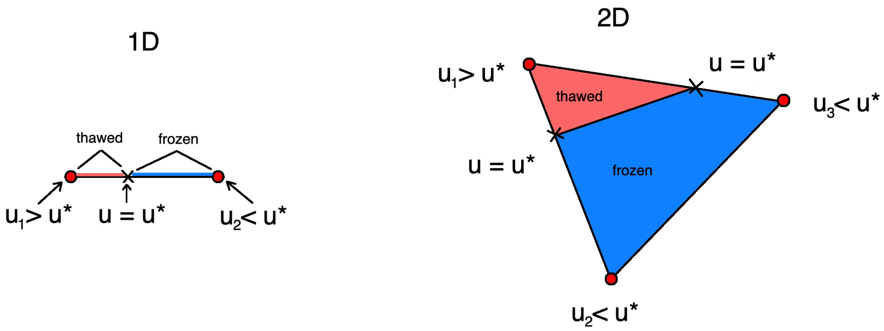
5.1. One-Dimensional Problem

The computational domain size $L=8 \mathrm{m}$. We simulate for $T={10}^7 \mathrm{s}$ with initial condition:

$$u_0(x)=u_0,\hspace{1em}t=0,\hspace{1em}x\in [0,L],$$

with $u_0=5{ }^{\circ }$C.

The boundary conditions are the following:

$$u(0,t)=g,\hspace{1em}\frac{\partial u}{\partial x}(L,t)=0,\hspace{1em}t>0,$$

where we consider two test cases with $g=-5{ }^{\circ }$C and $g=-15{ }^{\circ }$C.

For a one-dimensional problem, an exact solution of the two-phase Stefan problem is defined using the phase change interface location $\xi =\xi (t)$:

$$\xi =\gamma \sqrt{t},$$

where $\gamma$ is the coefficient of proportionality (m/s${}^{0.5}$).

The exact solution has the following form [13]:

$$u(x,t)=\left\{\begin{array}{cc}g\left[\mathrm{erf}\left(\frac{\xi }{2a_1\sqrt{t}}\right)-\mathrm{erf}\left(\frac{x}{2a_1\sqrt{t}}\right)\right]/\mathrm{erf}\left(\frac{\xi }{2a_1\sqrt{t}}\right),\hfill & x\ge \xi (t),\hfill \\ u_0\left[\mathrm{erf}\left(\frac{x}{2a_2\sqrt{t}}\right)-\mathrm{erf}\left(\frac{\xi }{2a_2\sqrt{t}}\right)\right]/\left[1-\mathrm{erf}\left(\frac{\xi }{2a_2\sqrt{t}}\right)\right],\hfill & x<\xi (t).\hfill \end{array}\right.$$

Using a phase change interface condition (2), we find $\gamma$ as the root of the transcendental equation:

$$\frac{k_1}{a_1}g\frac{exp\left(-{\left(\frac{\gamma }{2a_1}\right)}^2\right)}{\mathrm{erf}\left(\frac{\gamma }{2a_1}\right)}+\frac{k_2}{a_2}{u}_0\frac{exp\left(-{\left(\frac{\gamma }{2a_2}\right)}^2\right)}{1-\mathrm{erf}\left(\frac{\gamma }{2a_2}\right)}+\gamma D\frac{\sqrt{\pi }}{2}=0,$$

where $a_1=\sqrt{k_1/c_1}, a_2=\sqrt{k_2/c_2}$, and $\mathrm{erf}$ is the error function [13,14,15,16]. The value of $\gamma$ is calculated using the iterative secant method with the accuracy of $ϵ<{10}^{-12}$. We have $\gamma =0.00023897230346$ for $g=-5$ and $\gamma =0.0004188066281859222$ for $g=-15$.

In Figure 2, we present exact and numerical solutions at the final time $T={10}^7 \mathrm{s}\approx 115$ days and a phase change interface location $\xi (t)$. We present the results of the numerical solution of the problem using three types of smoothing. Numerical calculations were performed with $n=200$ (mesh by space) and $m=200$ for the time approximation. We consider the case with $g=-5{ }^{\circ }$C and $g=-15{ }^{\circ }$C. The smoothing parameter is chosen constant $\Delta =0.3$ throughout the entire computation time $t\in (0,T]$. In the left figure, a solution at the final time is presented, where we see that the first derivative of the function has a discontinuity of the first kind with respect to spatial variable x at $u=u^{*}$, which agrees with the Stefan condition. In the right figure, we depict a phase change interface location by time. In numerical calculations, the phase change interface is found through the linear interpolation method in the interval, where the sought function has different signs at the ends $(u_i^m·u_{i+1}^m)<0$. We observe that the numerical solution both for the temperature at the final time and for the phase change interface location is accurate for smoothing using error functions (erf-smoothing) and for smoothing in one spatial interval (h-smoothing). We note that the novel method based on smoothing in one spatial interval is more accurate than the scheme with approximation using the $\Delta$ parameter, that is, in general, it should be carefully chosen for each test case and depends on the mesh size, number of time steps, and speed of the phase change interface propagation.

Next, we investigate the influence of the mesh size and the number of time steps on the accuracy of the presented methods. We consider $n=25,50,100,200$ for the spatial mesh and $m=50,100,200$ for the time approximation. We perform simulations and calculate errors for two smoothing parameters $\Delta =0.3$ and $\Delta =0.6$ in the erf-smoothing and delta-smoothing methods. We calculate the relative $L_2$ errors for a solution and phase change interface:

$$e_e(u_T)=\sqrt{\frac{{\sum }_i{(y_i(T)-u(x_i,T))}^2}{{\sum }_{i}u{(x_i,T)}^2}}\times 100\%,\hspace{1em}{e}_f(u_T)=\sqrt{\frac{{\sum }_i{(y_i(T)-{\tilde{u}}_i(T))}^2}{{\sum }_i{({\tilde{u}}_i(T))}^2}}\times 100\%,$$

$$e_e(\gamma )=\sqrt{\frac{{\sum }_j{({\xi }_j-{\xi }_e(t_j))}^2}{{\sum }_j{\xi }_e{(t_j)}^2}}\times 100\%,\hspace{1em}{e}_f(\gamma )=\sqrt{\frac{{\sum }_j{({\xi }_j-{\xi }_f(t_j))}^2}{{\sum }_j{\xi }_f{(t_j)}^2}}\times 100\%,$$

where $y,\xi$ are the numerical solutions, $u(x,t),{\xi }_e(t)$ are the exact solutions, and $\tilde{u},{\xi }_f$ are the solutions on the very fine grid with $n=m=800$.

In

Table 1. One-dimensional problem with erf-smoothing. Relative $L_2$ error for the temperature at the final time and phase change interface location with respect to the exact solution and a very fine grid solution.

$\mathit{g}=-5$
n	m	${\mathit{e}}_{\mathit{e}}({\mathit{u}}_{\mathit{T}})$	${\mathit{e}}_{\mathit{e}}(\mathit{\gamma })$	${\mathit{e}}_{\mathit{f}}({\mathit{u}}_{\mathit{T}})$	${\mathit{e}}_{\mathit{f}}(\mathit{\gamma })$
$\Delta =0.3$
25	50	8.665	57.564	9.786	57.766
50	50	7.962	53.930	9.059	54.133
100	50	0.603	9.985	1.195	10.152
200	50	1.657	1.209	0.468	1.146
25	100	5.747	36.560	6.781	36.752
50	100	3.625	30.125	4.752	30.310
100	100	1.116	1.575	0.291	1.718
200	100	1.478	0.889	0.238	0.783
25	200	2.039	13.374	2.889	13.517
50	200	2.194	19.971	3.285	20.147
100	200	1.755	18.043	2.709	18.220
200	200	1.059	2.812	0.346	2.963
$\Delta =0.6$
25	50	4.364	11.751	3.196	11.694
50	50	3.463	4.871	1.206	4.781
100	50	3.253	2.253	0.532	2.169
200	50	3.125	0.900	0.299	0.883
25	100	4.536	13.432	3.293	13.367
50	100	3.660	6.740	1.330	6.633
100	100	2.813	2.559	0.278	2.616
200	100	3.059	0.738	0.170	0.674
25	200	4.510	13.737	3.278	13.670
50	200	3.561	6.637	1.219	6.529
100	200	3.199	2.567	0.386	2.450
200	200	3.072	0.924	0.147	0.806
$\Delta =0.3$
25	50	29.267	85.669	30.360	87.115
50	50	24.491	68.825	25.694	70.129
100	50	2.556	2.614	1.691	2.923
200	50	3.855	4.075	2.880	3.587
25	100	12.403	34.199	13.338	35.294
50	100	6.643	24.756	7.729	25.782
100	100	3.129	14.451	4.188	15.393
200	100	2.387	2.329	1.309	1.982
25	200	2.641	16.891	3.888	17.781
50	200	8.379	31.700	9.514	32.780
100	200	7.077	24.754	8.161	25.780
200	200	1.805	1.509	0.612	1.098
$\Delta =0.6$
25	50	5.451	5.759	5.157	5.718
50	50	3.335	3.963	1.644	4.004
100	50	3.883	3.273	2.051	3.235
200	50	3.968	2.998	2.025	2.815
25	100	3.851	6.643	3.920	6.910
50	100	1.587	9.790	1.916	10.239
100	100	2.811	2.737	0.625	2.966
200	100	3.396	2.268	1.166	1.992
25	200	5.495	8.275	5.050	8.042
50	200	3.332	4.132	1.616	3.848
100	200	3.196	2.468	0.908	2.192
200	200	3.054	1.555	0.594	1.253

,

Table 2. One-dimensional problem with h-smoothing. Relative $L_2$ error for the temperature at the final time and phase change interface location with respect to the exact solution and a very fine grid solution.

$\mathit{g}=-5$
n	m	${\mathit{e}}_{\mathit{e}}({\mathit{u}}_{\mathit{T}})$	${\mathit{e}}_{\mathit{e}}(\mathit{\gamma })$	${\mathit{e}}_{\mathit{f}}({\mathit{u}}_{\mathit{T}})$	${\mathit{e}}_{\mathit{f}}(\mathit{\gamma })$
25	50	1.841	5.102	1.651	5.647
50	50	0.824	2.902	0.641	3.497
100	50	0.519	2.864	0.326	3.415
200	50	0.960	1.726	0.766	1.481
25	100	1.686	5.060	1.504	5.596
50	100	0.610	2.580	0.448	3.177
100	100	0.374	1.598	0.179	2.204
200	100	0.490	1.051	0.302	1.447
25	200	1.750	4.555	1.567	5.035
50	200	0.616	2.131	0.454	2.703
100	200	0.352	1.142	0.157	1.729
200	200	0.156	0.813	0.049	1.326
$\mathit{g}=-\mathbf{15}$
n	m	${\mathit{e}}_{\mathit{e}}({\mathit{u}}_{\mathit{T}})$	${\mathit{e}}_{\mathit{e}}(\mathit{\gamma })$	${\mathit{e}}_{\mathit{f}}({\mathit{u}}_{\mathit{T}})$	${\mathit{e}}_{\mathit{f}}(\mathit{\gamma })$
25	50	0.467	8.617	1.478	10.688
50	50	0.821	4.320	0.521	6.231
100	50	1.794	2.198	0.565	3.629
200	50	4.215	4.275	2.979	3.140
25	100	0.544	7.970	1.557	9.978
50	100	0.827	3.373	0.507	5.273
100	100	1.739	1.308	0.476	1.469
200	100	1.896	1.700	0.645	1.308
25	200	0.557	7.558	1.504	9.549
50	200	0.426	3.459	0.915	5.404
100	200	0.740	1.450	0.545	3.282
200	200	0.910	0.799	0.356	1.649

and

Table 3. One-dimensional problem with delta-smoothing. Relative $L_2$ error for temperature at the final time and phase change interface location with respect to the exact solution and a very fine grid solution.

$\mathit{g}=-5$
n	m	${\mathit{e}}_{\mathit{e}}({\mathit{u}}_{\mathit{T}})$	${\mathit{e}}_{\mathit{e}}(\mathit{\gamma })$	${\mathit{e}}_{\mathit{f}}({\mathit{u}}_{\mathit{T}})$	${\mathit{e}}_{\mathit{f}}(\mathit{\gamma })$
$\Delta =0.3$
25	50	19.718	90.023	20.149	88.656
50	50	8.422	39.373	8.826	38.419
100	50	2.789	20.121	3.178	19.112
200	50	1.228	11.510	1.560	10.564
25	100	4.133	20.358	4.559	19.400
50	100	3.817	25.213	4.255	24.123
100	100	4.897	33.164	5.303	32.035
200	100	3.086	24.004	3.467	22.928
25	200	3.801	15.419	4.188	14.540
50	200	5.337	37.751	5.809	36.612
100	200	2.102	13.071	2.411	12.129
200	200	0.431	6.272	0.745	5.244
$\Delta =0.6$
25	50	8.393	31.522	9.007	30.953
50	50	1.764	2.935	1.257	2.982
100	50	0.957	9.480	1.298	8.953
200	50	0.868	5.798	0.668	5.290
25	100	3.388	12.386	3.494	12.402
50	100	2.153	9.925	2.511	9.401
100	100	3.092	25.393	3.997	24.806
200	100	1.195	1.599	0.189	1.069
25	200	2.873	10.084	3.473	9.805
50	200	2.238	9.417	2.589	8.893
100	200	1.369	1.684	0.296	2.024
200	200	1.117	2.739	0.305	2.189
$\mathit{g}=-\mathit{15}$
n	m	${\mathit{e}}_{\mathit{e}}({\mathit{u}}_{\mathit{T}})$	${\mathit{e}}_{\mathit{e}}(\mathit{\gamma })$	${\mathit{e}}_{\mathit{f}}({\mathit{u}}_{\mathit{T}})$	${\mathit{e}}_{\mathit{f}}(\mathit{\gamma })$
$\Delta =0.3$
25	50	55.431	102.593	55.776	102.265
50	50	43.798	104.751	44.197	104.378
100	50	3.391	9.541	3.651	9.250
200	50	0.774	4.601	1.077	4.341
25	100	30.288	69.374	30.599	69.026
50	100	16.591	46.798	16.940	46.499
100	100	3.516	9.969	3.798	9.654
200	100	2.262	7.067	2.513	6.768
25	200	2.343	7.735	2.730	7.711
50	200	16.595	48.645	16.944	48.349
100	200	15.455	42.005	15.826	41.679
200	200	0.880	3.063	1.046	2.723
$\Delta =0.6$
25	50	31.869	63.799	32.609	63.736
50	50	1.384	5.835	1.789	5.774
100	50	0.655	3.723	1.154	3.659
200	50	1.179	2.218	0.364	2.154
25	100	3.711	19.023	4.782	18.960
50	100	8.162	19.368	8.695	19.299
100	100	3.725	12.748	4.387	12.681
200	100	1.294	6.778	1.675	6.710
25	200	2.821	7.808	3.557	7.752
50	200	8.437	24.475	9.144	24.414
100	200	1.143	1.521	0.402	1.451
200	200	1.113	1.113	0.276	1.032

, we present the relative errors for the three methods: erf-smoothing, h-smoothing, and linear delta-smoothing. We present relative errors in % and investigate the influence of the boundary condition, smoothing interval $\Delta$, and the space and time mesh parameters on the accuracy of the numerical solution. In Table 1, the relative errors for the scheme with smoothing using an error function are presented (erf-smoothing) for $\Delta =0.3$ and $\Delta =0.6$, where errors for $g=-5$ are presented on the left and for $g=-15$ presented on the right. In Table 2, the results for the scheme with smoothing in one spatial interval (h-smoothing) are presented. Relative errors for the scheme with linear smoothing on the $\Delta$ interval are presented in Table 3 (h-smoothing) for $\Delta =0.3$ and $\Delta =0.6$. From the errors between the exact and numerical solutions ($e_e(u_T)$ and $e_e(\gamma )$), we observe that the erf-smoothing and linear delta-smoothing methods are highly dependent on parameter $\Delta$. The error decreases along with the spatial mesh refining as the number of time layers increases.

The errors between a very fine grid solution ($m=n=800$) and a numerical solution for different parameters m and n ($e_f(u_T)$ and $e_f(\gamma )$) demonstrate the convergence of the solution depending on m and n. We observe that for the coarse parameters m and n, we can obtain results with a large error. For example, we have $e_f(u_T)=25\%$ and $e_f(\gamma )=70\%$ for $\Delta =0.3$, $g=-15$, and $m=n=50$ for the erf-smoothing method. For larger $\Delta$, we can obtain more stable results. However, for a finer mesh and more time steps, the parameter $\Delta =0.6$ is too large to obtain good approximation. For example, we have $e_f(u_T)=3\%$ for $\Delta =0.6$ and $e_f(u_T)=1\%$ for $\Delta =0.3$ in the test problem with $g=-5$ and $m=n=200$. A new method with smoothing in one spatial interval (h-smoothing) does not have parameter $\Delta$ and provides very good results with small errors and convergence depending on parameters m and n. This method automatically determines a sufficient smoothing parameter.

A graphical illustration of the errors from Table 1, Table 2 and Table 3 for the presented methods is shown in Figure 3 and Figure 4. We depict errors for $m=100$ and $m=200$ with different spatial mesh parameters n and $\Delta$. The h-smoothing scheme provides accurate results on a coarse spatial grid at large time steps. We observe that the erf-smoothing method is less sensitive to the parameter $\Delta$ and provides sufficiently good results with a good choice of the parameter $\Delta$. By comparing the results for $g=-5$ and $g=-15$ in Figure 3 and Figure 4, we see that for a larger temperature gradient, we obtain worse results. In the erf-smoothing and delta-smoothing methods, we should use a finer mesh and more time steps for better approximation with a good choice of parameter $\Delta$. The scheme with smoothing in one spatial interval provides an accurate numerical solution with the minimal smoothing interval, which is different in each spatial interval and time layer.

5.2. Two-Dimensional Problem

In this section, we present numerical results for a two-dimensional heat problem. We consider the two-phase Stefan problem with similar parameters as in the previous section. We consider computational domain $\mathrm{\Omega }=[L_1\times L_2]$ with size $L_1=L_2=2 \mathrm{m}$ and simulate for $T={10}^6 \mathrm{s}$ with initial condition $u_0=5{ }^{\circ }$C. As boundary conditions, we set $g=-5{ }^{\circ }$C and $g=-15{ }^{\circ }$C for $x\in {\mathrm{\Gamma }}_1=\{x\in \partial \mathrm{\Omega }:x=0, y=0\}$ and zero flux on other boundaries, $\partial \mathrm{\Omega }/{\mathrm{\Gamma }}_1$. The computational mesh is uniform with triangular cells with size $n=n_1\times n_2$. Numerical calculations are performed with $m=200$ for the time approximation. We present the results of the numerical solution of the problem using three types of smoothing schemes for $n=n_1\times n_2$, $n_1=n_2=25,50,100$, and 100.

We calculate relative $L_2$ errors for the solution at the final time:

$$e_e(u_T)=\sqrt{\frac{{\sum }_i{(y_i(T)-u_{f,hs}(x_i,T))}^2}{{\sum }_i{u}_{f,hs}{(x_i,T)}^2}},\hspace{1em}{e}_f(u_T)=\sqrt{\frac{{\sum }_i{(y_i(T)-{\tilde{u}}_i(T))}^2}{{\sum }_i{({\tilde{u}}_i(T))}^2}},$$

where y is the numerical solution and $\tilde{u}$ is the solution on the fine grid with $n=m=400$ using the current method. Here, for $u_{f,hs}(x,T)$, we use a reference solution with the h-smoothing method. We compare the results with h-smoothing to show that this method provides an accurate solution and does not depend on the parameter $\Delta$ as in the previous examples for the one-dimensional problem.

In Figure 5, we present the numerical solution at the final time for $g=-5{ }^{\circ }$C and $g=-15{ }^{\circ }$C. In the left figure, we depict a temperature field at the final time with an isotherm of $u=u^{*}$ (phase change interface). In the right figure, we show a solution on line $x_1=x_2$, where the line is depicted in yellow color in the left figure. The phase change interface at the final time is depicted for three types of smoothing and indicated in different colors. Here, we use a similar color in the right figure to plot the temperature along the line $x_1=x_2$. Numerical calculations are performed with $n=200$ (mesh by space) and $m=200$ for the time approximation. The smoothing parameter is chosen as constant $\Delta =0.3$.

In

Table 4. Two-dimensional problem with erf-smoothing. Relative $L_2$ error for the temperature at the final time with respect to the finest grid solution using the presented method ($e_f(u_T)$) and h-smoothing ($e_e(u_T)$).

$\mathit{g}=-5$
n	m	${\mathit{e}}_{\mathit{e}}({\mathit{u}}_{\mathit{T}})$	${\mathit{e}}_{\mathit{f}}({\mathit{u}}_{\mathit{T}})$
$\Delta =0.15$
25 × 25	200	6.671	6.430
50 × 50	200	4.252	4.073
100 × 100	200	1.540	1.079
200 × 200	200	1.211	0.329
$\Delta =0.3$
25 × 25	200	7.339	6.083
50 × 50	200	4.714	2.957
100 × 100	200	3.851	1.467
200 × 200	200	3.263	0.552
$\Delta =0.6$
25 × 25	200	9.585	5.538
50 × 50	200	7.472	2.080
100 × 100	200	7.022	1.036
200 × 200	200	6.554	0.281
$\mathit{g}=-\mathit{15}$
n	m	${\mathit{e}}_{\mathit{e}}({\mathit{u}}_{\mathit{T}})$	${\mathit{e}}_{\mathit{f}}({\mathit{u}}_{\mathit{T}})$
$\Delta =0.15$
25 × 25	200	3.409	3.664
50 × 50	200	1.633	1.598
100 × 100	200	1.259	1.923
200 × 200	200	2.059	1.226
$\Delta =0.3$
25 × 25	200	4.206	4.484
5 × 500	200	1.567	1.348
100 × 100	200	2.360	2.426
200 × 200	200	1.967	1.376
$\Delta =0.6$
25 × 25	200	6.636	6.360
50 × 50	200	4.368	3.427
100 × 100	200	3.891	2.013
200 × 200	200	3.738	0.833

,

Table 5. Two-dimensional problem with h-smoothing. Relative $L_2$ error for the temperature at the final time with respect to the finest grid solution using the presented method ($e_f(u_T)=e_e(u_T)$).

$\mathit{g}=-5$
n	m	${\mathit{e}}_{\mathit{e}}({\mathit{u}}_{\mathit{T}})$	${\mathit{e}}_{\mathit{f}}({\mathit{u}}_{\mathit{T}})$
25 × 25	200	4.338	4.338
50 × 50	200	1.760	1.760
100 × 100	200	0.574	0.574
200 × 200	200	0.178	0.178
$\mathit{g}=-\mathit{15}$
n	m	${\mathit{e}}_{\mathit{e}}({\mathit{u}}_{\mathit{T}})$	${\mathit{e}}_{\mathit{f}}({\mathit{u}}_{\mathit{T}})$
25 × 25	200	2.078	2.078
50 × 50	200	1.293	1.293
100 × 100	200	1.029	1.029
200 × 200	200	0.145	0.145

and

Table 6. Two-dimensional problem with delta-smoothing. Relative $L_2$ error for the temperature at the final time with respect to the finest grid solution using the presented method ($e_f(u_T)$) and h-smoothing ($e_e(u_T)$).

$\mathit{g}=-5$
n	m	${\mathit{e}}_{\mathit{e}}({\mathit{u}}_{\mathit{T}})$	${\mathit{e}}_{\mathit{f}}({\mathit{u}}_{\mathit{T}})$
$\Delta =0.15$
25 × 25	200	6.151	5.598
50 × 50	200	11.598	10.937
100 × 100	200	10.485	9.836
200 × 200	200	7.338	6.668
$\Delta =0.3$
25 × 25	200	3.647	3.818
50 × 50	200	3.782	3.556
100 × 100	200	4.261	3.951
200 × 200	200	1.374	0.919
$\Delta =0.6$
25 × 25	200	4.748	4.148
50 × 50	200	3.968	2.340
100 × 100	200	3.153	0.486
200 × 200	200	3.146	0.304
$\mathit{g}=-\mathit{15}$
n	m	${\mathit{e}}_{\mathit{e}}({\mathit{u}}_{\mathit{T}})$	${\mathit{e}}_{\mathit{f}}({\mathit{u}}_{\mathit{T}})$
$\Delta =0.15$
25 × 25	200	27.421	20.040
50 × 50	200	27.005	19.437
100 × 100	200	25.048	17.213
200 × 200	200	9.524	2.822
$\Delta =0.3$
25 × 25	200	12.662	9.941
50 × 50	200	18.554	15.872
100 × 100	200	15.926	13.138
200 × 200	200	5.139	2.203
$\Delta =0.6$
25 × 25	200	2.991	2.856
50 × 50	200	4.883	3.217
100 × 100	200	1.968	0.909
200 × 200	200	2.121	0.692

, we investigate the influence of the mesh size (n) on the accuracy of the presented methods. Time step number m is fixed, $m=200$. We consider $n=25,50,100,200$ for the spatial mesh. In Table 4, we present the relative errors for the erf-smoothing scheme with $\Delta =0.15,0.3$, and $0.6$. In the left table, we present the errors for boundary condition $g=-5$. The table at the right demonstrates the results for $g=-15$. We present relative errors in % and investigate the influence of mesh size on the accuracy of the numerical solution. In Table 5, the results for the h-smoothing scheme are presented for $g=-5$ and $-15$. Relative errors for delta-smoothing are shown in Table 6. The first error $e_e(u_T)$ is an error between the current solution and a reference solution using the h-smoothing scheme on mesh $m=n=400$. We observe that in order to obtain good results using the erf-smoothing scheme, we should take smaller $\Delta$ for $g-5$ than for the test case with $g=-15$. For example, we have $6.5\%$ of the error for $\Delta =0.6$ and $1.2\%$ of the error for $\Delta =0.15$ in the test case with $g=-5$. Table 6 shows the optimal value of $\Delta =0.3$ for $g=-5$ and $\Delta =0.6$ for $g=-15$. For the h-smoothing scheme with smoothing in one spatial interval, we obtain good results for both test cases with $g=-5$ and $g=-15$.

The second error $e_f(u_T)$ illustrates the convergence of the solution with increasing mesh parameters m and n to the reference solution on the fine grid $m=n=400$ using the corresponding method. We observe that both errors $e_f(u_T)$ and $e_e(u_T)$ are sensitive to the size of the mesh, where we obtain a large error for a very coarse grid $n_1=n_2=25$. We obtain accurate results for $n=50,100$, and 100 using the h-smoothing method.

5.3. Geometry with an Unstructured Grid

The main advantage of the finite element method is that it provides the possibility of problem solving in complex geometries using the construction of the unstructured mesh with triangular elements.

We consider the computational domain with size $L_1=6 \mathrm{m}$ with a rough boundary and two circle perforations. In Figure 6, we depict the computational domain and unstructured mesh. In the left figure, we present the computational domain. The unstructured grid with triangular elements is presented in the right figure. We depict a rough top boundary ${\mathrm{\Gamma }}_1$ in green color, where we set the Dirichlet boundary conditions:

$$u(x,t)=g,\hspace{1em}x\in {\mathrm{\Gamma }}_1.$$

Similar to the previous results, we consider $g=-5$ and $g=-15$. On the circle perforation, we set the Robin-type boundary conditions:

$$-k\frac{\partial u}{\partial x}(x,t)=\alpha (u-g_1),\hspace{1em}x\in {\mathrm{\Gamma }}_{t1},\hspace{1em}-k\frac{\partial u}{\partial x}(x,t)=\alpha (u-g_2),\hspace{1em}x\in {\mathrm{\Gamma }}_{t2},$$

where we set $\alpha =20$. In Figure 6, the first circle is indicated in red color with $g_1=10$, and the second circle is indicated in orange color with $g_2=15$. Circle perforations illustrate a pipe influence to the temperature distribution. The pipes contain fluid with temperature $g_1$ (first) and $g_2$ (second) with heat transfer parameter $\alpha$. The radius of the first circle is $r_1=0.1$, and the radius of the second one is $r_2=0.2$. On other boundaries (blue color), we set the Neumann boundary condition:

$$-k\frac{\partial u}{\partial x}(x,t)=0,\hspace{1em}x\in \partial \mathrm{\Omega }/({\mathrm{\Gamma }}_1\cup {\mathrm{\Gamma }}_{t1}\cup {\mathrm{\Gamma }}_{t1}.$$

We simulate for $T={10}^6 \mathrm{s}$ with initial condition $u_0=2{ }^{\circ }$C. A computational mesh is fixed and contains n vertices, $n=$ 18,242.

The numerical solution at the final time for $g=-5{ }^{\circ }$C and $g=-15{ }^{\circ }$C is presented in Figure 7 and Figure 8, respectively. In the left figure, we depict the temperature field at the final time with the isotherm of $u=u^{*}$ (phase change interface). In the right figure, we show the solution on lines $x_1=2.5$ (line position is indicated in yellow color in the left figure) and $x_1=4.2$ (orange color in the left figure). The phase change interface at the final time is depicted for three types of smoothing in different colors in the left figure, and we use a similar color in the right figure to plot the temperature along lines. Numerical calculations are performed for $\Delta =0.3$ with $m=200$ for the time approximation.

We calculate similar errors for the solution at the final time ($e_e(u_T)$ and $e_f(u_T)$). The error $e_f(u_T)$ is calculated using the solution with $m=400$ using the current method. The error $e_f(u_T)$ is calculated using the reference solution with the h-smoothing method. In

Table 7. Geometry with unstructured grid with delta-smoothing. Relative $L_2$ error for the temperature at the final time and phase change interface location with respect to the exact solution and a very fine grid solution.

$\mathit{g}=-5$
n	m	${\mathit{e}}_{\mathit{e}}({\mathit{u}}_{\mathit{T}})$	${\mathit{e}}_{\mathit{f}}({\mathit{u}}_{\mathit{T}})$
$\Delta =0.15$
18,242	50	1.753	0.589
18,242	100	1.871	0.443
18,242	200	1.857	0.301
$\Delta =0.3$
18,242	50	3.052	0.825
18,242	100	3.249	0.322
18,242	200	3.366	0.086
$\Delta =0.6$
18,242	50	7.075	0.960
18,242	100	7.286	0.430
18,242	200	7.407	0.144
$\mathit{g}=-\mathit{15}$
n	m	${\mathit{e}}_{\mathit{e}}({\mathit{u}}_{\mathit{T}})$	${\mathit{e}}_{\mathit{f}}({\mathit{u}}_{\mathit{T}})$
$\Delta =0.15$
18,242	50	3.934	3.257
18,242	100	3.087	2.318
18,242	200	1.923	1.007
$\Delta =0.3$
18,242	50	2.487	1.759
18,242	100	2.192	1.189
18,242	200	1.894	0.548
$\Delta =0.6$
18,242	50	3.422	0.797
18,242	100	3.499	0.486
18,242	200	3.534	0.210

,

Table 8. Geometry with the unstructured grid with h-smoothing. Relative $L_2$ error for the temperature at the final time and phase change interface location with respect to the exact solution and a very fine grid solution.

$\mathit{g}=-5$
n	m	${\mathit{e}}_{\mathit{e}}({\mathit{u}}_{\mathit{T}})$	${\mathit{e}}_{\mathit{f}}({\mathit{u}}_{\mathit{T}})$
18,242	50	0.877	0.877
18,242	100	0.515	0.515
18,242	200	0.196	0.196
$\mathit{g}=-\mathit{15}$
n	m	${\mathit{e}}_{\mathit{e}}({\mathit{u}}_{\mathit{T}})$	${\mathit{e}}_{\mathit{f}}({\mathit{u}}_{\mathit{T}})$
18,242	50	3.355	3.355
18,242	100	1.992	1.992
18,242	200	0.821	0.821

and

Table 9. Geometry with the unstructured grid with delta-smoothing. Relative $L_2$ error for the temperature at the final time and phase change interface location with respect to the exact solution and a very fine grid solution.

$\mathit{g}=-5$
n	m	${\mathit{e}}_{\mathit{e}}({\mathit{u}}_{\mathit{T}})$	${\mathit{e}}_{\mathit{f}}({\mathit{u}}_{\mathit{T}})$
$\Delta =0.15$
18,242	50	2.833	1.361
18,242	100	2.684	0.909
18,242	200	2.357	0.570
$\Delta =0.3$
18,242	50	1.556	0.721
18,242	100	1.500	0.376
18,242	200	1.500	0.167
$\Delta =0.6$
18,242	50	2.941	0.951
18,242	100	3.032	0.401
18,242	200	3.113	0.105
$\mathit{g}=-\mathit{15}$
n	m	${\mathit{e}}_{\mathit{e}}({\mathit{u}}_{\mathit{T}})$	${\mathit{e}}_{\mathit{f}}({\mathit{u}}_{\mathit{T}})$
$\Delta =0.15$
18,242	50	3.832	2.351
18,242	100	4.459	1.009
18,242	200	4.356	0.892
$\Delta =0.3$
18,242	50	1.489	2.190
18,242	100	1.132	1.221
18,242	200	1.416	0.500
$\Delta =0.6$
18,242	50	1.510	1.177
18,242	100	1.483	0.647
18,242	200	1.552	0.273

, we investigate the influence of the number of time steps m and $\Delta$ on the accuracy of the presented methods. We consider $m=50,100,200$ and $\Delta =0.15,0.3,0.6$.

In Table 7, we present relative errors for the erf-smoothing scheme with $\Delta =0.15,0.3$, and $0.6$. In the left table, we present errors for boundary condition $g=-5$. In the right table, results for $g=-15$ are shown. In Table 8, the results for the h-smoothing scheme are presented for $g=-5$ and $-15$. The relative errors for delta-smoothing are shown in Table 9 for different values of m and $\Delta$. We observe good results for the erf-smoothing scheme, when we take $\Delta =0.15$ for $g=-5$ and $\Delta =0.3$ for $g=-15$. In the delta-smoothing scheme, we have good results for $\Delta =0.3$ for $g=-5$ and $g=-15$. We obtain an accurate solution for the scheme with h-smoothing for $m=50,100$, and 200 for $g=-5$ with less then one percent of error. The scheme with h-smoothing works very well for $g=-15$ with less than one percent for $m=200$.

We present and investigate three schemes: smoothing on the $\Delta$ interval using the error function (erf-smoothing), linear smoothing on the $\Delta$ interval (delta-smoothing), and smoothing in one mesh cell (h-smoothing). The first algorithm (erf-smoothing) is based on the analytical spreading of the point source function and smoothing of discontinuous coefficients. The algorithm with smoothing in one mesh cell (h-smoothing) provides a minimal length of the smoothing interval that is calculated automatically for the given temperature values on the mesh at a given time layer. The third scheme (delta-smoothing) is a convenient scheme based on smoothing using linear approximation on the $\Delta$ interval. We study the proposed schemes on one-dimensional and two-dimensional model problems. We consider a problem with two values of the boundary conditions on different spatial and time meshes. We present errors for the methods with smoothing on the $\Delta$ interval for different values of the smoothing interval parameter $\Delta$, which is fixed and given as a constant value. Numerical results show that the smoothing scheme with the minimal smoothing interval shows its computational efficiency and provides good results.

6. Conclusions

In this work, we consider the two-phase Stefan problem, which describes the heat transfer problems with phase change. In a two-phase formulation, the mathematical model is defined in the whole domain, which contains frozen and thawed zones.

The main problem is associated with the sharp phase change interface. For the numerical solution of the problem, we present and investigate schemes with smoothing in one spatial interval (cell) and smoothing on the $\Delta$ interval using the linear function and the error function. We observe that smoothing with the error function provides better results with smaller errors than linear smoothing on the $\Delta$ interval. However, the novel smoothing on one spatial interval (cell) gives better results, does not depend on the parameter $\Delta$, and can automatically smooth the coefficient in one mesh cell. We generalize the presented methods for the two-dimensional formulation of the problem and present results for two geometries with structured and unstructured meshes.

References

1. Samarsky, A.; Moiseenko, B. Economical shock-capturing scheme for multidimensional Stefan problems. Comput. Math. Math. Phys. 1965, 5, 816–827. [Google Scholar]
2. Budak, B.M.; Sobol’eva, E.; Uspenskii, A.B. A difference method with coefficient smoothing for the solution of Stefan problems. USSR Comput. Math. Math. Phys. 1965, 5, 59–76. [Google Scholar] [CrossRef]
3. Morgan, K.; Lewis, R.; Zienkiewicz, O. An improved algrorithm for heat conduction problems with phase change. Int. J. Numer. Methods Eng. 1978, 12, 1191–1195. [Google Scholar] [CrossRef]
4. Nedjar, B. An enthalpy-based finite element method for nonlinear heat problems involving phase change. Comput. Struct. 2002, 80, 9–21. [Google Scholar] [CrossRef]
5. Jäntschi, L.; Bolboacă, S.D. First order derivatives of thermodynamic functions under assumption of no chemical changes revisited. J. Comput. Sci. 2014, 5, 597–602. [Google Scholar] [CrossRef]
6. Danilyuk, I. On the Stefan problem. Russ. Math. Surv. 1985, 40, 157. [Google Scholar] [CrossRef]
7. Vasil’ev, V. Numerical Integration of Differential Equations with Nonlocal Boundary Conditions. Yakutsk. Fil. Sib. Otd. Akad. Nauk. SSSR Yakutsk. 1985. [Google Scholar]
8. Vasil’ev, V.; Maksimov, A.; Petrov, E.; Tsypkin, G. Heat and mass transfer in freezing and thawing soils. Nauk. Fizmatlib M 1996. [Google Scholar]
9. Samarskii, A.A.; Vabishchevich, P.N. Computational Heat Transfer; Wiley: Hoboken, NJ, USA, 1995. [Google Scholar]
10. Amiri, E.A.; Craig, J.R.; Hirmand, M.R. A trust region approach for numerical modeling of non-isothermal phase change. Comput. Geosci. 2019, 23, 911–923. [Google Scholar] [CrossRef]
11. Chessa, J.; Smolinski, P.; Belytschko, T. The extended finite element method (XFEM) for solidification problems. Int. J. Numer. Methods Eng. 2002, 53, 1959–1977. [Google Scholar] [CrossRef]
12. Vasilyeva, M.; Stepanov, S.; Spiridonov, D.; Vasil’ev, V. Multiscale Finite Element Method for heat transfer problem during artificial ground freezing. J. Comput. Appl. Math. 2020, 371, 112605. [Google Scholar] [CrossRef]
13. Tikhonov, A.N.; Samarskii, A.A. Equations of Mathematical Physics; Courier Corporation: North Chelmsford, MA, USA, 2013. [Google Scholar]
14. Neumann, F. Lectures Given in the 1860’s. Die Partiellen Differential-Gleichungen der Mthematischen Physik; 1912; Volume 2, pp. 17–121. [Google Scholar]
15. Lunardini, V.J. Heat Transfer with Freezing and Thawing; Elsevier: Amsterdam, The Netherlands, 1991. [Google Scholar]
16. Kurylyk, B.L.; McKenzie, J.M.; MacQuarrie, K.T.; Voss, C.I. Analytical solutions for benchmarking cold regions subsurface water flow and energy transport models: One-dimensional soil thaw with conduction and advection. Adv. Water Resour. 2014, 70, 172–184. [Google Scholar] [CrossRef]
Figure 1. Illustration of unfrozen water concentration η in mesh cell K i . Left: one-dimensional formulation (1D). Right: two-dimensional formulation (2D).
Mathematics 08 01924 g001
Figure 2. One-dimensional problem. Exact solution (black color). Numerical solutions using error function (erf) smoothing (blue color), smoothing in one spatial interval (red color), and linear smoothing in the Δ interval (green color). Left: solution at the final time. Right: phase change interface location.
Mathematics 08 01924 g002
Figure 3. One-dimensional problem. Boundary conditions g = 5 . Numerical solutions using error function smoothing (blue color), smoothing in one spatial interval (red color), and linear smoothing using the Δ interval (green color). Solid line for m = 200 and dashed line for m = 100 . Left: relative L 2 errors for the solution at the final time. Right: relative L 2 errors for the phase change interface location.
Mathematics 08 01924 g003
Figure 4. One-dimensional problem. Boundary conditions g = 5 . Numerical solutions using error function smoothing (blue color), smoothing in one spatial interval (red color), and linear smoothing using the Δ interval (green color). Solid line for m = 200 and dashed line for m = 100 . Left: relative L 2 errors for the solution at the final time. Right: relative L 2 errors for the phase change interface location.
Mathematics 08 01924 g004
Figure 5. Two-dimensional problem. Numerical solutions using error function smoothing (blue color), smoothing in one spatial interval (red color), and linear smoothing using the Δ interval (green color). Left: solution at the final time. Right: solution on line x 1 = x 2 at the final time.
Mathematics 08 01924 g005
Figure 6. Geometry with unstructured grid. Left: computational domain (gray color), top boundary (green), circle one (red), and circle two (orange). Right: unstructured mesh with triangular elements.
Mathematics 08 01924 g006
Figure 7. Geometry with the unstructured grid for g = 5 . Numerical solutions using error function smoothing (blue color), smoothing in one spatial interval (red color), and linear smoothing using the Δ interval (green color). Yellow line: x 1 = 2.5 . Orange line: x 1 = 4.2 .
Mathematics 08 01924 g007
Figure 8. Geometry with the unstructured grid for g = 5 . Numerical solutions using error function smoothing (blue color), smoothing in one spatial interval (red color), and linear smoothing using the Δ interval (green color). Yellow line: x 1 = 2.5 . Orange line: x 1 = 4.2 .
Mathematics 08 01924 g008