A New HWMA Dispersion Control Chart with an Application to Wind Farm Data ^†

Abstract

Recently, a homogeneously weighted moving average (HWMA) chart has been suggested for the efficient detection of small shifts in the process mean. In this study, we have proposed a new one-sided HWMA chart to effectively detect small changes in the process dispersion. The run-length (RL) profiles like the average RL, the standard deviation RL, and the median RL are used as the performance measures. The RL profile comparisons indicate that the proposed chart has a better performance than its existing counterpart’s charts for detecting small shifts in the process dispersion. An application related to the Dhahran wind farm data is also part of this study.

1. Introduction

In every industrial environment, product quality is affected by the variation in the manufacturing process. The presence of variation in the manufacturing processes is quite obvious, which blemishes the product’s quality characteristics. To maintain the product quality, it is necessary to monitor the changes that occur due to assignable causes. Control charts are very popular statistical process monitoring (SPM) tools used to monitor the changes that occur due to assignable causes. There are two main types of control charts: memory-less and memory-type control charts. Memory-type control charts have received much attention in modern era industries to handle the unusual variations in the parameters of the distribution of manufacturing/service process characteristics. The cumulative sum (CUSUM) and the exponentially weighted moving average (EWMA) introduced by References [1,2] respectively, are frequently used memory-type charts, and the most commonly used memory-less charts are the Shewhart charts proposed by Reference [3].

Generally, assignable causes affect both the process mean and variance. A process can go to an out-of-control (OOC) process if the mean is shifted to another level. Likewise, an increase in variance can also cause inconsistency in the process [4]. In real-life applications, it is essential to monitor the process output for early detection of deviation in process parameters, i.e., mean and variance. However, we prefer to stabilize the variance first, as we know the mean structure depends on it, and also the decrease in variance leads to an enhancement in the process production [5].

The transformation of the sample variance ($S^2)$ is the most useful procedure to monitor the process variance. The authors of Reference [6] suggest a one-sided EWMA chart by adopting the log transformation on $S^2$, labeled as the ${\mathrm{CH}}_{\mathrm{E}}$ chart. The S²-EWMA and S²-CUSUM charts were introduced by References [7] and [8] by applying the three parametric logarithmic transformations on $S^2$. The one-sided CH-EWMA chart was suggested in Reference [9] by applying the truncating log transformation on $S^2$ and is hereafter named the ${\mathrm{SJ}}_{\mathrm{E}}$ chart. The work of Reference [10] suggested the one-sided EWMA chart to monitor the increase in the process variance and labeled this chart as the H-EWMA chart. The CS-EWMA and mixed CUSUM-EWMA (S²-MCE) charts were suggested in References [11] and [12] by applying the same transformation used in Reference [7]. Motivated by Reference [11], the authors of Reference [13] introduced a mixture of generally weighted moving average (GWMA) and CUSUM charts for monitoring small deviations in the process variance.

Recently, a homogeneously weighted moving average (HWMA) chart was proposed in Reference [14] to overcome the deficiency in the EWMA chart statistic. Numerous works have been done with the HWMA chart due to its earlier shift detection ability in the process mean as compared to the EWMA chart. The authors of References [15,16] developed the auxiliary information-based HWMA chart and multivariate form of the HWMA chart. The HWMA chart using the neoteric ranked set sampling was proposed in Reference [17]. To enhance the HWMA chart’s performance, a double HWMA chart for efficient monitoring of the process mean was suggested in Reference [18]. The literature mentioned above on the HWMA chart has only monitored the changes in the process mean. To the best of our knowledge, no work has been done in the SPM literature to monitor the changes in the process variance under the HWMA chart scenario. In this study, we fill this gap and suggest a HWMA chart to evaluate the changes in the process variance.

Moreover, most industrial and manufacturing processes are usually affected by the increase in the process variance. The increase in the process variance deteriorates the performance of the production processes. This study’s main objective is to propose an effective control chart that performs efficiently in the case of often increases in the process variance. So, inspired by Huwang et al. [10] and Abbas [14], we suggest a one-sided HWMA chart to monitor the changes in the increase of the process variance, hereafter labeled as ${\mathrm{SJ}}_{\mathrm{H}}$. To evaluate the performance of the ${\mathrm{SJ}}_{\mathrm{H}}$ chart, we have used various run-length (RL) profiles like the average RL (ARL), the standard deviation RL (SDRL), and the median RL (MDRL). A chart having a larger value of in-control ($\mathrm{IC})$ $\mathrm{ARL},$ i.e., ${\mathrm{ARL}}_0,$ and a smaller value of $\mathrm{OOC}$ $\mathrm{ARL},$ i.e., ${\mathrm{ARL}}_1$ is considered to be efficient.

The other sections of this article are in the following sequence: In Section 2, we provide the suggested chart’s proposal. The tabulated and graphical comparisons are offered in Section 3. Real-life applications are provided in Section 4. In Section 5, conclusions are drawn based on findings from this research

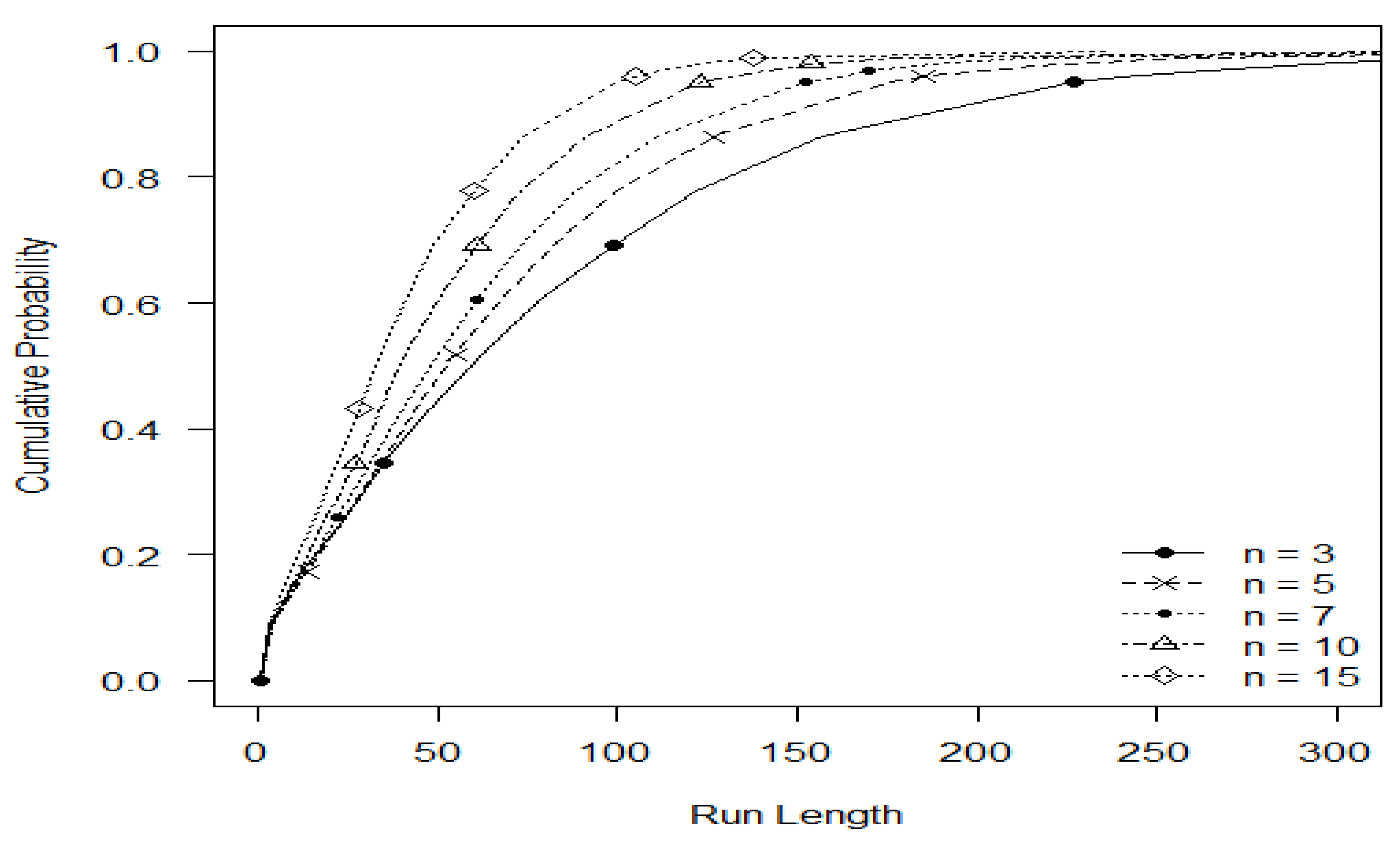
2. Design and Performance Evaluation of the Proposed Chart

Let us assume that $X_{t1},X_{t2}, . . ., X_{tn}$ be $n$ independent and identically distributed normal random variables with mean ${\mu }_t$ and variance ${\sigma }_t^2,$ i.e., $X_{ti}~N\left({\mu }_t, {\sigma }_t^2\right)$ for, $i=1, 2, 3, . . ., n$, where ${\sigma }_t^2={\sigma }_0^2$ for an IC process, and let ${\sigma }_t^2\ne {\sigma }_0^2$ for an OOC process. Let $\tau ={\sigma }_t/{\sigma }_0$ be the ratio of the OOC and IC standard deviations. For an IC process, $\tau =1$, and for an OOC process, $\tau \ne 1$. Without loss of generality, we have assumed that ${\mu }_t=0$. Let ${\overline{X}}_t$ and $S_t^2$ be the sample mean and sample variance at time $t$, respectively. Let $Y_t=ln\left(S_t^2/{\sigma }_0^2\right)$. The distribution of the random variable $S_t^2/{\sigma }_0^2$ is the gamma distribution with shape $\left(n-1\right)/2$ and scale $2{\delta }_t^2/\left(n-1\right)$, and the parameters and the distribution of $Y_t$ is log-gamma distribution. Later on, the authors of Reference [19] showed that $Y_t$ is approximately normally distributed with mean ${\mu }_Y$ and variance ${\sigma }_Y^2$, where

$${\mu }_Y\approx ln\left({\delta }_t^2\right)-\frac{1}{n-1}-\frac{1}{3{\left(n-1\right)}^2}+\frac{2}{15{\left(n-1\right)}^4} \mathrm{and} {\sigma }_Y^2\approx \frac{2}{n-1}+\frac{2}{{\left(n-1\right)}^2}+\frac{4}{3{\left(n-1\right)}^3}-\frac{16}{15{\left(n-1\right)}^5}.$$

Let the sample mean of $Y_t$ be defined as: $Z_t=\frac{{{\displaystyle \sum }}_{i=1}^n{Y}_{ti}}{n}$. Motivated from Reference [10], the statistic of the suggested ${\mathrm{SJ}}_{\mathrm{H}}$ chart is defined as:

$$H_t=max\left(\lambda Z_t + \left(1-\lambda \right){\overline{Z}}_{t-1},0\right)$$

(1)

where $\lambda \in (0, 1]$ is the smoothing constant and ${\overline{Z}}_{t-1},$ is the mean of all the previous $Z_t \mathrm{values}.$ It is defined as ${\overline{Z}}_{t-1}=\frac{{{\displaystyle \sum }}_{i=1}^{t-1}{Z}_i}{t-1}$. We consider ${\overline{Z}}_0=0$. The statistic given in (1) can also be defined as:

$$H_t=max\left[\lambda Z_t +\left\{\left(\frac{1-\lambda }{t-1}\right)Z_{t-1}+\left(\frac{1-\lambda }{t-1}\right)Z_{t-2}+\dots +\left(\frac{1-\lambda }{t-1}\right)Z_1\right\} ,0\right]$$

(2)

The ${\mathrm{SJ}}_{\mathrm{H}}$ chart triggers an OOC signal if $H_t$ is greater than

$$UC{L}_t=\begin{array}{c} C_t\sqrt{\frac{{\lambda }^2{\sigma }_Y^2}{n}} if t=1\\ C_t\sqrt{\frac{{\lambda }^2{\sigma }_Y^2}{n}+{\left(1-\lambda \right)}^2\frac{{\sigma }_Y^2}{n\left(t-1\right)} }, if t>1\end{array}$$

(3)

and it indicates the increase in the process variance, where $C_t$ is the width of the control limits and can be chosen to achieve the desired ${\mathrm{ARL}}_0$.

So many methods are available, like integral equations, Markov chains, and Monte Carlo (MC) simulations, to calculate the $\mathrm{ARL}$. We have performed MC simulations to evaluate the $\mathrm{ARL}$ of the ${\mathrm{SJ}}_{\mathrm{H}}$ chart because this method is more accurate than the integral equations and Markov chain methods [13]. The flow chart for the computation of the $\mathrm{ARL}$ of the ${\mathrm{SJ}}_{\mathrm{H}}$ chart is given in Figure 1.

The$\mathrm{RL}$ profiles’ values of the proposed ${\mathrm{SJ}}_{\mathrm{H}}$ chart are provided in

Table 1. The RL profiles of the proposed chart under various choices of $\lambda$ for $n=5$.

$\mathit{\tau }$	RL Characteristic	$\mathit{\lambda }$
		0.05	0.1	0.2	0.3	0.5
1	ARL	199.90	201.42	201.47	202.11	202.38
	MDRL	113.00	154.00	149.00	146.00	141.50
	SDRL	246.86	182.73	183.48	188.57	200.84
1.05	ARL	50.04	65.53	73.66	77.56	89.27
	MDRL	29.00	51.00	58.00	58.00	64.00
	SDRL	58.62	57.67	61.46	69.86	85.98
1.1	ARL	22.25	32.47	37.57	39.39	45.93
	MDRL	12.00	26.00	30.00	31.00	33.00
	SDRL	25.80	27.70	30.35	33.26	42.84
1.2	ARL	8.78	13.68	15.88	16.19	18.14
	MDRL	5.00	11.00	13.00	13.00	14.00
	SDRL	9.61	11.82	12.25	12.82	16.05
1.3	ARL	5.15	7.66	9.11	9.44	9.89
	MDRL	4.00	6.00	8.00	8.00	8.00
	SDRL	5.14	6.63	6.78	7.20	8.38
1.4	ARL	3.64	5.20	6.23	6.40	6.45
	MDRL	3.00	4.00	5.00	5.00	5.00
	SDRL	3.35	4.30	4.55	4.73	5.19
1.5	ARL	2.86	3.93	4.62	4.65	4.68
	MDRL	2.00	3.00	4.00	4.00	4.00
	SDRL	2.40	3.16	3.38	3.38	3.67
1.6	ARL	2.40	3.16	3.71	3.67	3.67
	MDRL	1.00	3.00	3.00	3.00	3.00
	SDRL	1.96	2.46	2.64	2.58	2.70
1.7	ARL	2.12	2.66	3.08	3.08	3.05
	MDRL	1.00	2.00	3.00	3.00	3.00
	SDRL	1.65	2.01	2.14	2.11	2.17
1.8	ARL	1.88	2.32	2.64	2.66	2.61
	MDRL	1.00	1.00	2.00	2.00	2.00
	SDRL	1.43	1.70	1.85	1.83	1.81
1.9	ARL	1.74	2.08	2.33	2.32	2.27
	MDRL	1.00	1.00	2.00	2.00	2.00
	SDRL	1.24	1.51	1.60	1.56	1.49
2	ARL	1.57	1.91	2.10	2.10	2.05
	MDRL	1.00	1.00	1.00	2.00	2.00
	SDRL	1.09	1.35	1.40	1.37	1.30
$C_t$		1.3	1.932	2.402	2.55	2.65

for selective choices of $\lambda$ by fixing ${\mathrm{ARL}}_0\approx 200$. From Table 1, it is observed that if we increase the value of $\lambda ,$ the ${\mathrm{ARL}}_1$ values of the ${\mathrm{SJ}}_{\mathrm{H}}$ chart decrease, and vice versa (for example, when ${\delta }_t=1.1, \lambda =0.05, {\mathrm{ARL}}_1=22.25 \mathrm{vs}. {\delta }_t=1.1,$ $\lambda =0.5, {\mathrm{ARL}}_1=45.93$). The MDRL values are smaller than ARL values which specify that the distribution of the RL is positively skewed (Table 1). The SDRL values are decreased as the value of ${\delta }_t$ increases (for example, when ${\delta }_t=0, \lambda =0.05, \mathrm{SDRL}=246.86 \mathrm{vs}. {\delta }_t=1.2,$ $\lambda =0.5, \mathrm{SDRL}=9.61$ (Table 1)). We have also checked the performance of the proposed ${\mathrm{SJ}}_{\mathrm{H}}$ chart for various choices of $n$ and it is reported in

Table 2. The RL profiles of the proposed chart under various choices of $n$ for $\lambda =0.1.$

$\mathit{\tau }$	RL Characteristic	$\mathit{n}$
		3	5	7	10	15
1	ARL	202.85	201.42	198.01	198.44	196.41
	MDRL	143	154	153	158	155
	SDRL	209.11	182.73	176.45	170.88	167.69
1.05	ARL	80.57	65.53	56.92	47.78	39.4
	MDRL	60	51	46	39	33
	SDRL	77.68	57.67	48.25	39.29	31.72
1.1	ARL	43.9	32.47	26.54	21.37	16.12
	MDRL	33	26	22	18	13
	SDRL	41.44	27.7	22.2	17.61	13.21
1.2	ARL	19.48	13.68	10.32	7.71	5.83
	MDRL	14.5	11	8	6	5
	SDRL	18.45	11.82	8.7	6.28	4.58
1.3	ARL	11.67	7.66	5.88	4.41	3.22
	MDRL	8	6	5	4	3
	SDRL	10.84	6.63	4.76	3.45	2.35
1.4	ARL	8.14	5.2	3.96	3.02	2.25
	MDRL	6	4	3	3	1
	SDRL	7.54	4.3	3.11	2.24	1.56
1.5	ARL	6.05	3.93	3.01	2.33	1.77
	MDRL	4	3	3	1	1
	SDRL	5.5	3.16	2.26	1.65	1.17
1.6	ARL	4.9	3.16	2.48	1.91	1.49
	MDRL	4	3	2	1	1
	SDRL	4.34	2.46	1.78	1.3	0.91
1.7	ARL	4.06	2.66	2.1	1.64	1.31
	MDRL	3	2	1	1	1
	SDRL	3.51	2.01	1.47	1.06	0.73
1.8	ARL	3.62	2.32	1.83	1.47	1.18
	MDRL	3	1	1	1	1
	SDRL	3.05	1.7	1.27	0.9	0.56
1.9	ARL	3.15	2.08	1.65	1.34	1.11
	MDRL	3	1	1	1	1
	SDRL	2.6	1.51	1.09	0.77	0.44
2	ARL	2.81	1.91	1.5	1.25	1.07
	MDRL	2	1	1	1	1
	SDRL	2.25	1.35	0.95	0.66	0.35
$C_t$		1.591	1.932	2.09	2.215	2.32

. The ${\mathrm{ARL}}_1$ values of the ${\mathrm{SJ}}_{\mathrm{H}}$ chart decrease as the value of n is increased for a fixed choice of ${\delta }_t$ and $\lambda$ (for example, when ${\delta }_t=1.1, \lambda =0.05, n=3, {\mathrm{ARL}}_1=43.6 \mathrm{vs}. {\delta }_t=1.1,$ $\lambda =0.05, n=15, {\mathrm{ARL}}_1=16.12$). Moreover, the RL curves of the proposed ${\mathrm{SJ}}_{\mathrm{H}}$ chart are provided in Figure 2 and Figure 3 for various combinations of $\lambda \mathrm{and} n$. It is noted that as the value of $\lambda$ increases, the RL values of the ${\mathrm{SJ}}_{\mathrm{H}}$ chart are decreased for a fixed choice of $n$ and ${\delta }_t$ (Figure 2). From Figure 3, it is seen that as the value of $n$ increases, the RL values of the ${\mathrm{SJ}}_{\mathrm{H}}$ chart decrease or are fixed values of $\lambda$ and ${\delta }_t$.

3. Comparisons between Proposed and Existing Charts

The ${\mathrm{ARL}}_1$ comparisons of the proposed ${\mathrm{SJ}}_{\mathrm{H}}$ chart with the existing charts are provided in this sub-section. For comparison purposes, the following existing charts are included: ${\mathrm{CH}}_{\mathrm{E}}$, ${\mathrm{SJ}}_{\mathrm{E}}$, and H-EWMA proposed by References [6,9,10], respectively. The performance comparisons between proposed and existing charts are also judged by using another measure called the percentage decrease in $\mathrm{ARL}$, hereafter labeled as PD-ARL. The PD-ARL can be computed by using the formula $\left(\frac{AR{L}_0-AR{L}_1}{AR{L}_0}\right)\times 100$ [18]. A chart having a larger PD-ARL value is considered to be efficient. We have fixed the ${\mathrm{ARL}}_0$ at $200$ for valid comparisons.

To compare the ${\mathrm{ARL}}_1$ performance of the ${\mathrm{SJ}}_{\mathrm{H}}$ chart with existing charts, we have found the following interesting points:

• The ${\mathrm{ARL}}_1$ performance of the ${\mathrm{SJ}}_{\mathrm{H}}$ chart is relatively improved compared to the ${\mathrm{CH}}_{\mathrm{E}}$chart (for example, in the ${\mathrm{CH}}_{\mathrm{E}}$chart with $=0.05,$ ${\delta }_t=1.1, 1.2, 1.3, 1.4, \mathrm{and} 1.5$, ${\mathrm{ARL}}_1=43.24, 18.09, 10.77, 7.13, \mathrm{and} 5.98,$and in the ${\mathrm{SJ}}_{\mathrm{H}}$ chart for $\lambda =0.05$, ${\delta }_t=1.1, 1.2, 1.3, 1.4, \mathrm{and} 1.5$, ${\mathrm{ARL}}_1=22.25, 8.78, 5.15, 3.64, \mathrm{and} 2.86$ (Table 1 vs.

  Table 3. The ${\mathrm{ARL}}_1$ performance of the existing charts for various choices of $\lambda$ for $n=5.$

  $\mathit{\tau }$	$\mathit{\lambda }$
  	0.05			0.1			0.2			0.3
  	$\mathbf{C}{\mathbf{H}}_{\mathbf{E}}$	$\mathbf{S}{\mathbf{J}}_{\mathbf{E}}$	H-EWMA	$\mathbf{C}{\mathbf{H}}_{\mathbf{E}}$	$\mathbf{S}{\mathbf{J}}_{\mathbf{E}}$	H-EWMA	$\mathbf{C}{\mathbf{H}}_{\mathbf{E}}$	$\mathbf{S}{\mathbf{J}}_{\mathbf{E}}$	H-EWMA	$\mathbf{C}{\mathbf{H}}_{\mathbf{E}}$	$\mathbf{S}{\mathbf{J}}_{\mathbf{E}}$	H-EWMA
  1	200.33	200.75	200.92	200.02	200.36	199.51	200.64	199.48	199.43	199.4	199.67	200.22
  1.1	43.24	32.26	28.89	44.26	35.15	34.32	46.63	39.73	41.18	48.48	43.45	46.14
  1.2	18.09	14.43	11.69	18.23	14.96	14.1	18.79	16.05	16.66	19.52	17.25	18.65
  1.3	10.77	9.17	6.85	10.56	9.09	8.2	10.54	9.21	9.45	10.67	9.56	10.35
  1.4	7.63	6.73	4.75	7.35	6.53	5.65	7.16	6.4	6.45	7.09	6.43	6.9
  1.5	5.98	5.38	3.62	5.68	5.13	4.28	5.41	4.89	4.83	5.24	4.8	5.11
  1.6	4.96	4.51	2.94	4.68	4.27	3.46	4.38	3.99	3.86	4.2	3.88	4.06
  1.7	4.29	3.92	2.51	4.02	3.69	2.91	3.73	3.41	3.25	3.53	3.26	3.39
  1.8	3.8	3.5	2.2	3.56	3.27	2.53	3.27	3	2.81	3.06	2.83	2.91
  1.9	3.44	3.17	1.96	3.22	2.96	2.25	2.92	2.69	2.48	2.73	2.53	2.57
  2	3.18	2.93	1.8	2.95	2.72	2.03	2.67	2.45	2.24	2.47	2.3	2.32
  $C_t$	1.055	1.568	1.828	1.303	1.943	2.079	1.513	2.27	2.253	1.598	2.433	2.302

  )). Also, at ${\delta }_t=1.1$, the values of PD-ARL in ${\mathrm{CH}}_{\mathrm{E}}$ and ${\mathrm{SJ}}_{\mathrm{H}}$ charts are 78.38% and 88.87% respectively, for $\lambda =0.05$.
• The ${\mathrm{SJ}}_{\mathrm{H}}$ chart has an enhanced ${\mathrm{ARL}}_1$ performance over the ${\mathrm{SJ}}_{\mathrm{E}}$chart (for example, when $\lambda =0.05, \mathrm{and} {\delta }_t=1.1, 1.2, 1.3, 1.4,$ the ${\mathrm{ARL}}_1$ values of the ${\mathrm{SJ}}_{\mathrm{E}}$and ${\mathrm{SJ}}_{\mathrm{H}}$ charts are 32.26, 14.43, 9.17, 6.73 and $22.25, 8.78, 5.15, 3.64, 2.86$, respectively (Table 1 vs. Table 2)). Also, at ${\delta }_t=1.2$, the value of PD-ARL in the ${\mathrm{SJ}}_{\mathrm{E}}$chart is 92.52% but the value of PD-ARL in the ${\mathrm{SJ}}_{\mathrm{H}}$ chart is 93.16%, for $\lambda =0.1$.
• It is revealed that the ${\mathrm{ARL}}_1$ performance of the ${\mathrm{SJ}}_{\mathrm{H}}$ is quite efficient against the H-EWMA chart (for example, in the H-EWMA chart with $=0.05,$ ${\delta }_t=1.1, 1.3, 1.5$, ${\mathrm{ARL}}_1=28.89, 6.87, 3.62,$and in the ${\mathrm{SJ}}_{\mathrm{H}}$ chart for$\lambda =0.05$, ${\delta }_t=1.1, 1.3, 1.5$, and ${\mathrm{ARL}}_1=22.25, 5.15, 2.86$ (Table 1 vs. Table 3)). The PD-ARL values of the H-EWMA and ${\mathrm{SJ}}_{\mathrm{H}}$ charts are 79.11% and 81.26% respectively, with ${\delta }_t=1.1 \mathrm{and} \lambda =0.2.$

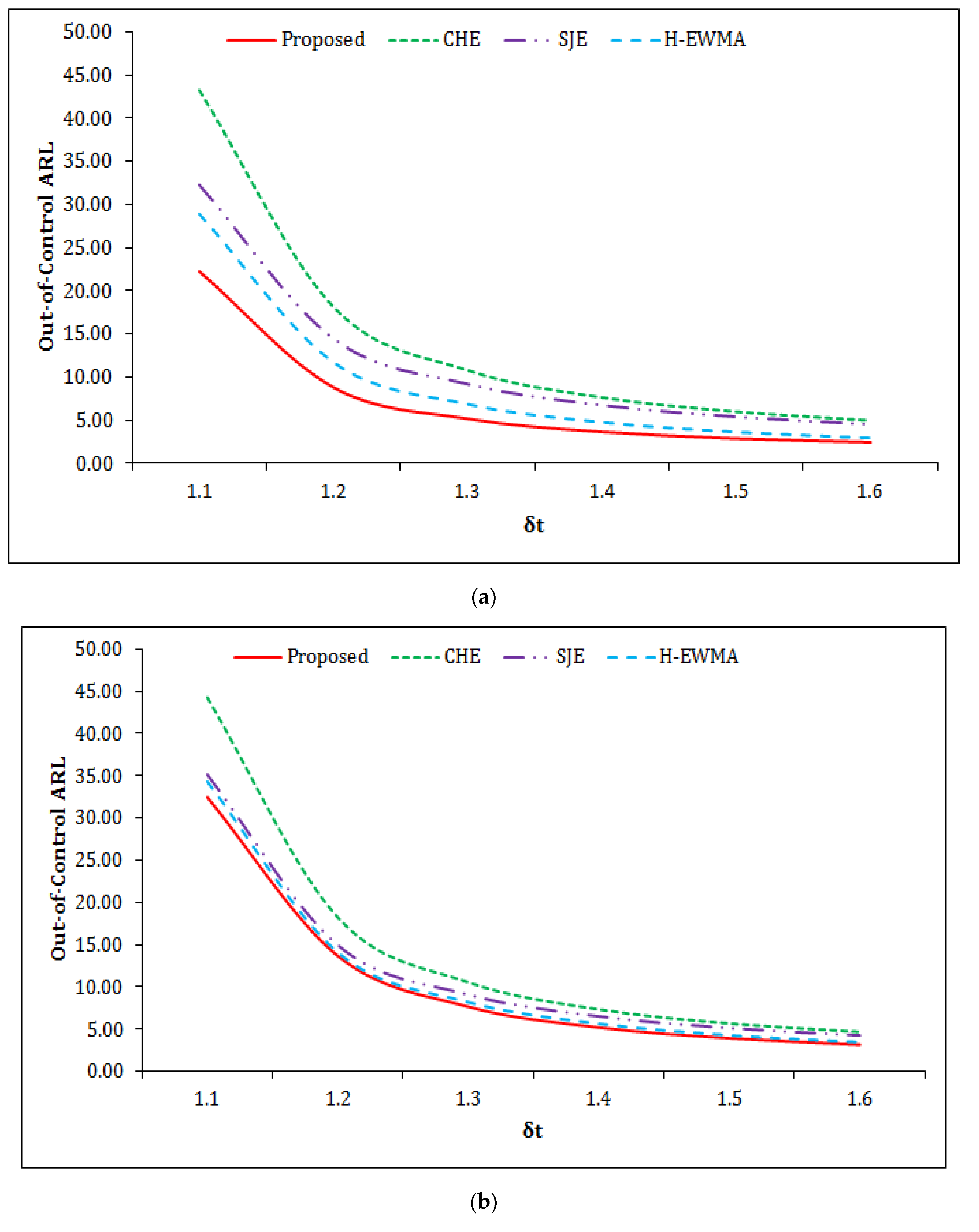
Graphical Comparisons between Proposed and Existing Charts

In this sub-section, we have also presented the ${\mathrm{ARL}}_1$-based graphical comparisons of the ${\mathrm{SJ}}_{\mathrm{H}}$ chart with the existing charts. From Figure 4a–d, it is noted that the performance of the proposed ${\mathrm{SJ}}_{\mathrm{H}}$ chart is relatively better than the ${\mathrm{CH}}_{\mathrm{E}}$, ${\mathrm{SJ}}_{\mathrm{E}}$, and H-EWMA charts for all selected choices of $\lambda$ and ${\delta }_t$. It is found that as the value of $\lambda$ increases the ${\mathrm{ARL}}_1,$ differences between the proposed ${\mathrm{SJ}}_{\mathrm{H}}$ and existing charts are decreased (Figure 4a–d). The performance of the ${\mathrm{SJ}}_{\mathrm{H}}$ is far better than the ${\mathrm{CH}}_{\mathrm{E}}$ and ${\mathrm{SJ}}_{\mathrm{E}}$ for selected choices of $\lambda$ under selected choices of ${\delta }_t$ (Figure 4a–d).

From tabulated and graphical comparisons, we have concluded that the ${\mathrm{SJ}}_{\mathrm{H}}$ chart performs well against the ${\mathrm{CH}}_{\mathrm{E}}$, ${\mathrm{SJ}}_{\mathrm{E}}$, and H-EWMA charts.

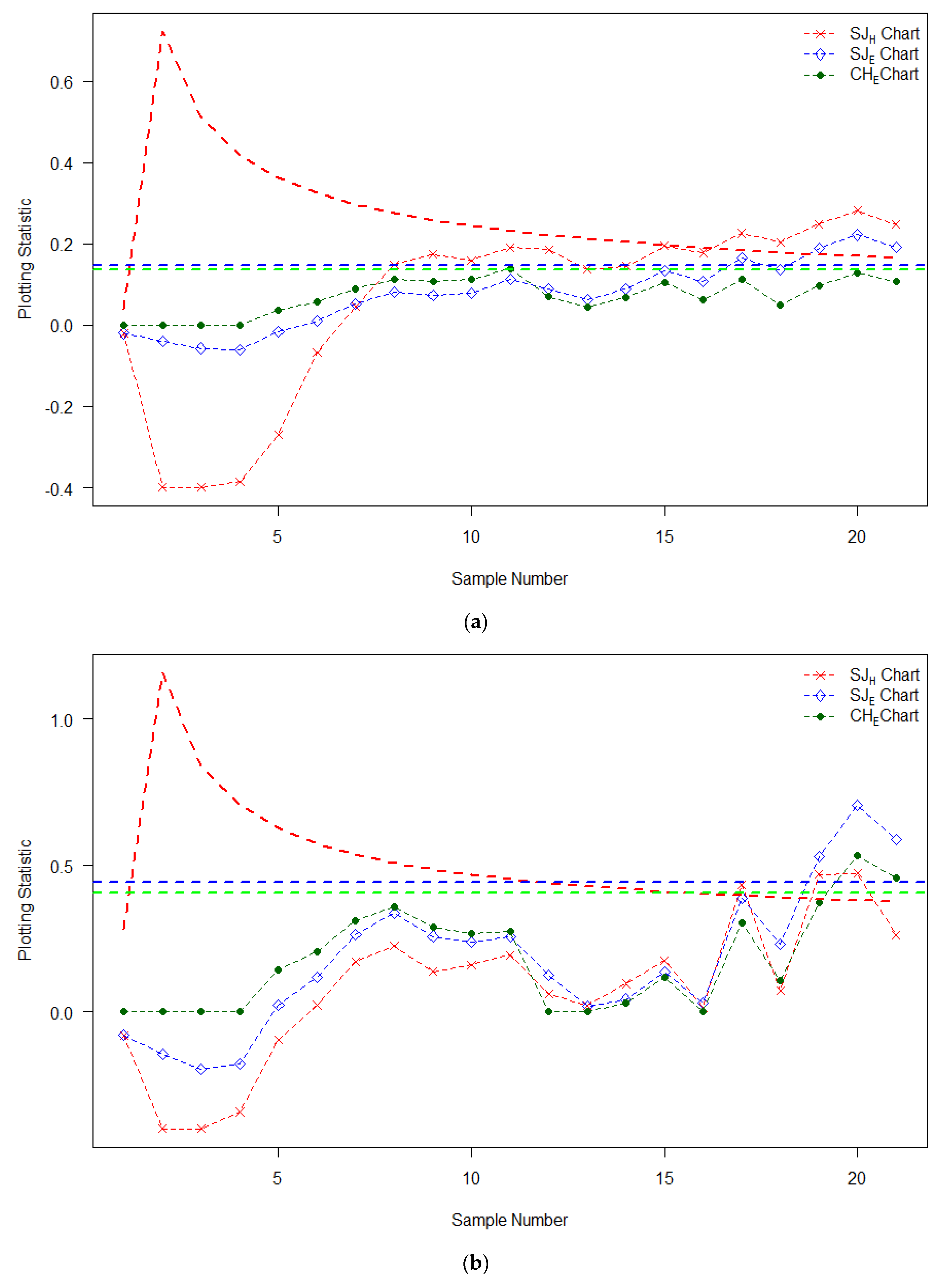
4. Application: Monitoring of Daily Power Generation at Dhahran Wind Farm

In this section, we present the application related to monitoring the daily power generated at the wind station located at the eastern coast of Dhahran (26°32′, 50°13′), Saudi Arabia. The daily energy generated was recorded during the winter period (15 November to 29 February 2020). The obtained data are given in

Table 4. The description of the wind farm data along with the plotting statistics of ${\mathrm{SJ}}_{\mathrm{H}}$, ${\mathrm{SJ}}_{\mathrm{E}}$, and ${\mathrm{CH}}_{\mathrm{E}}$.

Subgroup	${\mathit{X}}_1$	${\mathit{X}}_2$	${\mathit{X}}_3$	${\mathit{X}}_4$	${\mathit{X}}_5$	Example 1			Example 2
						$\mathbf{S}{\mathbf{J}}_{\mathbf{H}}$	$\mathbf{S}{\mathbf{J}}_{\mathbf{E}}$	$\mathbf{C}{\mathbf{H}}_{\mathbf{E}}$	$\mathbf{S}{\mathbf{J}}_{\mathbf{H}}$	$\mathbf{S}{\mathbf{J}}_{\mathbf{E}}$	$\mathbf{C}{\mathbf{H}}_{\mathbf{E}}$
1	0.6243	0.3376	−0.9172	0.0709	0.5376	−0.0199	−0.0199	0.0000	−0.0798	−0.0798	0.0000
2	0.0718	0.3996	−0.0596	1.3659	0.3227	−0.3989	−0.0389	0.0000	−0.3989	−0.1436	0.0000
3	−0.0353	−1.2937	−0.0296	0.0709	0.6338	−0.3989	−0.0569	0.0000	−0.3989	−0.1947	0.0000
4	−0.4403	−1.4717	0.0898	−0.4838	1.2130	−0.3847	−0.0598	0.0000	−0.3422	−0.1787	0.0000
5	−0.7443	−1.8528	−0.1009	0.9281	1.8177	−0.2703	−0.0155	0.0357	−0.0972	0.0222	0.1426
6	−1.1330	−1.6470	0.6685	1.3644	−0.6021	−0.0671	0.0105	0.0566	0.0231	0.1186	0.2051
7	−1.6013	−1.7784	0.6058	1.5148	0.2711	0.0450	0.0520	0.0901	0.1708	0.2632	0.3092
8	−1.3388	−1.4219	1.3121	1.1986	0.0989	0.1482	0.0810	0.1134	0.2244	0.3367	0.3587
9	−0.1471	−0.7052	0.6952	1.8248	−0.2702	0.1741	0.0740	0.1079	0.1375	0.2578	0.2877
10	0.4738	−1.2046	1.3146	1.5710	0.2134	0.1594	0.0785	0.1116	0.1601	0.2390	0.2664
11	−0.6251	−0.5070	2.4901	1.6751	−0.0464	0.1907	0.1136	0.1399	0.1931	0.2565	0.2756
12	−0.9566	−0.1195	−0.1200	0.4168	0.2475	0.1854	0.0880	0.0693	0.0601	0.1254	0.0000
13	−1.2295	0.8355	−0.9625	−0.2670	−0.4800	0.1367	0.0636	0.0434	0.0218	0.0206	0.0000
14	−0.5131	−0.8745	1.6919	−0.6865	−1.8279	0.1447	0.0897	0.0672	0.0954	0.0426	0.0310
15	0.6651	−0.3131	3.1758	−0.4326	−0.1728	0.1952	0.1335	0.1051	0.1742	0.1365	0.1170
16	0.8609	1.2055	0.7537	−0.5934	0.6171	0.1783	0.1069	0.0621	0.0145	0.0294	0.0000
17	−0.0632	−3.9879	−0.3150	−0.0427	−0.2883	0.2258	0.1652	0.1126	0.4340	0.3891	0.3036
18	−1.1750	−0.0632	−0.2966	0.2486	0.1488	0.2038	0.1370	0.0506	0.0707	0.2315	0.1070
19	−1.8194	−0.1347	2.6720	−0.3043	0.6523	0.2487	0.1886	0.0976	0.4695	0.5303	0.3727
20	−1.2295	−1.6588	1.8223	−1.1769	0.3310	0.2814	0.2219	0.1295	0.4724	0.7062	0.5346
21	−0.3456	−1.3377	0.7569	0.2470	0.6539	0.2474	0.1908	0.1081	0.2619	0.5895	0.4574

in the form of 21 subgroups, each of size 5, along with the plotting statistics of the charts considered for the application section.

Data Description

It is a tenable fact that the world is shifting focus from fossil fuels to renewable energy owing to CO₂ emission associated with fossil fuels during operation. Saudi Arabia subscribed to this initiative. Also, the increase in energy demand calls for the exploitation of other available cost-effective energy sources. Harnessing the readily available renewable energy sources such as wind and solar helps meet energy demand in a remote area and contributes significantly to the national grid. Extensive work has been carried out on wind data from various wind farms in the Kingdom; however, in the context of the control charts this is the first application. Wind speed data is available from different sources in the Kingdom. Among these are Saudi Aramco, Meteorology and Environmental Protection Administration (MEPA), and King Fahd University of Petroleum and Minerals (KFUPM) [20]. Wind power is the application of air flow through wind turbines to generate electric energy. The important parameter influencing the rate of energy generated in a wind farm are wind speed, wind direction, air temperature, and global solar radiation. Hourly metrological data was obtained from the meteorological monitoring station in the Eastern Province of Saudi Arabia [21]. The pictorial representation of the Dhahran wind farm is presented in Figure 5. We have also applied the Anderson Darling test to check the distribution of the Dhahran wind farm data, and from this test, it is observed that the distribution of the wind farm data is normal (Figure 6). We have considered the ${\mathrm{SJ}}_{\mathrm{H}}$, ${\mathrm{CH}}_{\mathrm{E}},$ and ${\mathrm{SJ}}_{\mathrm{E}}$ charts to possibly examine the deviations in the process variance by fixing ${\mathrm{ARL}}_0\approx 200$.

We have presented two examples based on wind farm data. In the first example, the first 10 subgroups are considered IC, and a shift of size 1.2 is introduced in the next 11 subgroups with $\lambda =0.05$ (Figure 7a). In the second example, the first 16 subgroups are considered IC, and a shift of size 1.5 is introduced in the next 5 subgroups with $\lambda =0.2$ (Figure 7b). The description of the wind farm data along with the plotting statistics of ${\mathrm{SJ}}_{\mathrm{H}}$, ${\mathrm{CH}}_{\mathrm{E}}$, and ${\mathrm{SJ}}_{\mathrm{E}}$ charts are reported in Table 4. From Figure 7a, it is seen that both the ${\mathrm{SJ}}_{\mathrm{H}}$ and ${\mathrm{SJ}}_{\mathrm{E}}$ charts trigger the $\mathrm{OOC}$ signal at the 17th subgroup point, whereas the ${\mathrm{CH}}_{\mathrm{E}}$ charts do not trigger any $\mathrm{OOC}$ signal. From Figure 7b, it is observed that the ${\mathrm{SJ}}_{\mathrm{H}}$ chart has detected the OOC signals at the 17th subgroup point. However, ${\mathrm{SJ}}_{\mathrm{E}}$ and ${\mathrm{CH}}_{\mathrm{E}}$ charts trigger the OOC signal at the 19th and 20th subgroup points, respectively. These illustrative examples clearly show the superiority of the ${\mathrm{SJ}}_{\mathrm{H}}$ chart as compared to the ${\mathrm{CH}}_{\mathrm{E}}$ and ${\mathrm{SJ}}_{\mathrm{E}}$ charts. The real life application also supported the findings in Section 3.

5. Concluding Remarks

The increase in the process variance deteriorates the performance of the production processes under consideration. In this study, we have suggested the ${\mathrm{SJ}}_{\mathrm{H}}$ chart for quickly and efficiently monitoring the changes in the upward increase of the process variance. Monte Carlo simulations were used to compute the various $RL$ profiles of the ${\mathrm{SJ}}_{\mathrm{H}}$ chart. The $RL$ profiles of the ${\mathrm{SJ}}_{\mathrm{H}}$ chart have been compared with ${\mathrm{CH}}_{\mathrm{E}}$, ${\mathrm{SJ}}_{\mathrm{E}}$, and H-EWMA charts. The $RL$ comparisons revealed that the ${\mathrm{SJ}}_{\mathrm{H}}$ chart shows superior performance compared with existing charts for monitoring upward shifts in the process dispersion. Hence, we recommend the practice of the ${\mathrm{SJ}}_{\mathrm{H}}$ chart to the SPM practitioners to monitor the upward shifts in the variance of a normally distributed process.

The scope of this study may be extended to develop efficient non-parametric and multivariate charts using the design structure of the ${\mathrm{SJ}}_{\mathrm{H}}$ chart.

References

1. Page, E.S. Continuous inspection schemes. Biometric 1954, 41, 100–115. [Google Scholar] [CrossRef]
2. Roberts, S.W. Control chart tests based on geometric moving averages. Technometrics 1959, 1, 239–250. [Google Scholar] [CrossRef]
3. Shewhart, W.A. Economic control of quality of manufactured product. Van Nostrand N. Y. 1932, 27, 215–217. [Google Scholar]
4. Montgomery, D.C. Introduction to Statistical Quality Control, 7th ed.; John Wiley & Sons: New York, NY, USA, 2011. [Google Scholar]
5. Domangue, R.; Patch, S.C. Some omnibus exponentially weighted moving average statistical process monitoring schemes. Technometrics 1991, 33, 299–313. [Google Scholar] [CrossRef]
6. Crowder, S.V.; Hamilton, M.D. An EWMA for monitoring a process standard deviation. J. Qual. Technol. 1992, 24, 12–21. [Google Scholar] [CrossRef]
7. Castagliola, P. A new S2-EWMA control chart for monitoring the process variance. Qual. Reliab. Eng. Int. 2005, 21, 781–794. [Google Scholar] [CrossRef]
8. Castagliola, P.; Celano, G.; Fichera, S. A new CUSUM-S2 control chart for monitoring the process variance. J. Qual. Mainte. Eng. 2009, 15, 344–357. [Google Scholar] [CrossRef]
9. Shu, L.; Jiang, W. A new EWMA chart for monitoring process dispersion. J. Qual. Technol. 2008, 40, 319–331. [Google Scholar] [CrossRef]
10. Huwang, L.; Huang, C.-J.; Wang, Y.-H.T. New EWMA control charts for monitoring process dispersion. Comput. Stat. Data Anal. 2010, 54, 2328–2342. [Google Scholar] [CrossRef]
11. Abbas, N.; Riaz, M.; Does, R.J.M.M. CS-EWMA chart for monitoring process dispersion. Qual. Reliab. Eng. Int. 2013, 29, 653–663. [Google Scholar] [CrossRef]
12. Zaman, B.; Abbas, N.; Riaz, M.; Lee, M.H. Mixed CUSUM-EWMA chart for monitoring process dispersion. Int. J. Adv. Manuf. Technol. 2016, 86, 3025–3039. [Google Scholar] [CrossRef]
13. Ali, R.; Haq, A. New GWMA-CUSUM control chart for monitoring the process dispersion. Qual. Reliab. Eng. Int. 2018, 34, 997–1028. [Google Scholar]
14. Abbas, N. Homogeneously weighted moving average control chart with an application in substrate manufacturing process. Comput. Ind. Eng. 2018, 120, 460–470. [Google Scholar] [CrossRef]
15. Adegoke, N.A.; Smith, A.N.H.; Anderson, M.J.; Sanusi, R.A.; Pawley, M.D.M. Efficient homogeneously weighted moving average chart for monitoring process mean using an auxiliary variable. IEEE Access 2019, 7, 94021–94032. [Google Scholar] [CrossRef]
16. Adegoke, N.A.; Abbasi, S.A.; Smith, A.N.H.; Anderson, M.J.; Pawley, M.D.M. A multivariate homogeneously weighted moving average control chart. IEEE Access 2019, 7, 9586–9597. [Google Scholar] [CrossRef]
17. Nawaz, T.; Han, D. Monitoring the process location by using new ranked set sampling based memory control charts. Qual. Technol. Quanti. Manag. 2020, 17, 255–284. [Google Scholar] [CrossRef]
18. Abid, M.; Shabbir, A.; Nazir, H.Z.; Sherwani, R.A.K.; Riaz, M. A double homogenously weighted moving average control chart for monitoring of the process mean. Qual. Reliab. Eng. Int. 2020, 36, 1513–1527. [Google Scholar] [CrossRef]
19. Lawless, J.F. Statistical Models and Methods for Lifetime Data, 2nd ed.; John Wiley & Sons: New York, NY, USA, 2003. [Google Scholar]
20. Said, S.A.; El-Amin, I.M.; Al-Shehri, A.M. Renewable energy potentials in Saudi Arabia. In Beirut regional Collaboration Workshop on Energy Efficiency and Renewable Energy Technology; American University of Beirut: Beirut, Lebanon, 2004; pp. 76–82. [Google Scholar]
21. Shaahid, S.M.; Elhadidy, M.A. Wind and solar energy at Dhahran, Saudi Arabia. Renew. Energy 1994, 4, 441–445. [Google Scholar] [CrossRef]
22. Wind Power Plant Project–Dumat Al Jandal. Available online: https://images.app.goo.gl/4t6QiQYvdDBYqehZ9 (accessed on 22 July 2019).
Figure 1. Flow chart procedure for the proposed chart.
Mathematics 08 02136 g001
Figure 2. Run-length (RL) curves for different levels of λ when n   =   5 and δ t = 1.2 .
Mathematics 08 02136 g002
Figure 3. Run-length curves for different levels of n when λ   =   0.05 and δ t = 1.05 .
Mathematics 08 02136 g003
Figure 4. The ARL 1 comparisons between proposed CH-EWMA, SJ-EWMA, and H-EWMA charts when (a) φ = 0.05 , (b) φ = 0.1 , (c) φ = 0.2 , and (d) φ = 0.3 .
Mathematics 08 02136 g004aMathematics 08 02136 g004b
Figure 5. Pictorial description of Dumat Al-Jandal wind farm [22].
Mathematics 08 02136 g005
Figure 6. Anderson-Darling normality test for Dhahran wind.
Mathematics 08 02136 g006
Figure 7. An application based on the wind farm data: (a) λ = 0.05 , (b) λ = 0.2 .
Mathematics 08 02136 g007