Abstract
For precise modeling of electromagnetic devices, we have to model material hysteresis. A Genetic Algorithm, Differential Evolution with three different strategies, teaching–learning-based optimization and Artificial Bee Colony, were used for testing seven different modified mathematical expressions, and the best combination of mathematical expression and solving method was used for hysteresis modeling. The parameters of the hysteresis model were determined based on the measured major hysteresis loop and first-order reversal curves. The model offers a simple determination of the magnetization procedure in the areas between measured curves, with the only correction of two parameters based on only two known points in the magnetization process. It was tested on two very different magnetic materials, and results show good agreement between the measured and calculated curves. The calculated curves between the measured curves have correct shapes. The main difference between our model and other models is that, in our model, each measured curve, major and reversal, is described with different parameters. The magnetization process between measured curves is described according to the nearest measured curve, and this ensures the best fit for each measured curve. In other models, there is mainly only one curve, a major hysteresis or magnetization curve, used for the determination of the parameters, and all other curves are then dependent on this curve. Results confirm that the evolutionary optimization method offers a reliable procedure for precise determination of the parameters.
1. Introduction
Precise modeling of electromagnetic devices helps us to develop energy-efficient devices. Modeling of modern electromagnetic devices is done mainly with the use of numerical models, such as the finite element model. To get a precise model that allows accurate modeling of electromagnetic devices, the description of the materials’ properties should be as good as possible. Often nonlinear magnetic material is described using a magnetization curve. To make a better material description and consider hysteresis losses, material hysteresis also has to be modeled. In the past, different hysteresis models were presented by different authors.
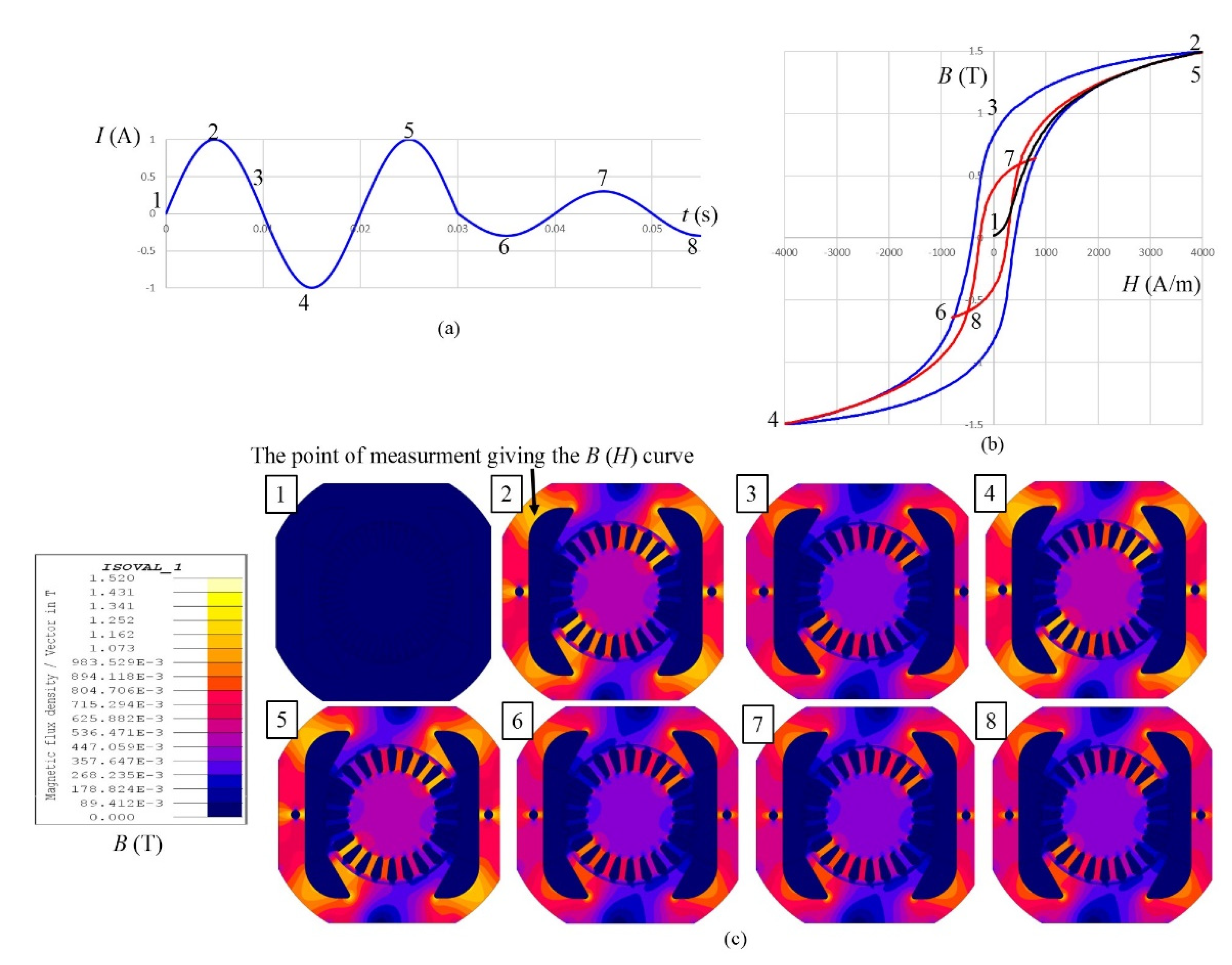
To understand the meaning of the hysteresis model better, the magnetization of the motor cross-section using hysteresis is presented schematically in Figure 1. The value of the excitation current (Figure 1a) changes from the value presented with point 1 to values in points 2, 3, … to point 8. Magnetization changes according to the curves presented between points marked at the hysteresis loop (Figure 1b) and appropriate magnetic flux density B at a cross-section of the motor for magnetization at each presented point (Figure 1c).

Figure 1.
Schematically presented magnetization using hysteresis: (a) Excitation current; (b) Hysteresis loop; (c) Magnetic flux density in the cross-section of the motor.
The magnetization process starts with demagnetized material at point 1. Magnetization from zero to the maximum current, point 2, is made using the original magnetization curve. From point 2 to point 4, magnetization is made according to the left part of the major hysteresis loop. From point 4 to point 5, magnetization is made according to the right part of the major hysteresis loop. For smaller current at points 6, 7 and 8, the magnetization is made according to the first-order reversal magnetization curves. The current can have any value, so the magnetization can be anywhere inside the hysteresis loop. Some of the first-order curves inside the hysteresis loop are measured, but most of them should be obtained using a hysteresis model.
Mathematical models can be classified into two main categories: physical and phenomenological. The former (physical model) is created from the physics of a phenomenon, while the latter merely describes the end result with mathematical functions. Therefore, the latter is usually less complex, but it loses the connection to the physics of the material. Among the physical models is the Stoner–Wohlfarth model [1], which is often used to describe events in ferromagnetic thin layers. The material is treated as a single magnetic domain. Jiles-Atherton [2,3,4], on the other hand, also considers inter-domain interactions. Their main advantage is the connection with the physical parameters. More numerically oriented is the Preisach model of hysteresis [5,6,7]. It enables the description of different forms of hysteresis loops that are constructed from the so-called hysterons. They can switch between −1 and 1, depending on whether the input data exceed the start-up or shut-off threshold. Other less known hysteresis models can be found, such as the Mayergoyz Vector Hysteresis model [8], or Vector Magneto–Hysteretic H&S model [9], and many modifications and corrections of existing models. The phenomenological, numerically oriented approach is presented in the paper.
The history of the magnetization process must also be known in the case of magnetic field calculation considering hysteresis. For the Finite Element Method (FEM) calculation [10,11,12,13,14,15,16,17,18,19,20], the magnetization process could be different for almost every element. Due to this fact, it is favorable that the description of the magnetization history is as simple as possible. It is expected that the model is suitable for a wide range of different materials. It is a challenging problem to determine the parameters of the hysteresis models.
In our work, a phenomenological scalar hysteresis model is made, which offers a simple description of the magnetization process. Different mathematical expressions are tested to get the most appropriate.
This test is possible only if a reliable tool to determine the parameters is available. Different evolutionary optimization methods were used for the determination of the parameters, with the aim to determine the best for such a problem. The improper determination of model parameters due to the improper selection of the optimization method can lead to an incorrect evaluation of model quality. The used methods were genetic algorithm (GA) [21,22,23,24,25,26], differential evolution (DE) with three different strategies, which are DE/rand/1/exp, DE/rand/2/exp, DE/best/1/bin [27,28,29,30,31,32,33,34,35,36], teaching–learning-based optimization (TLBO) [37,38,39,40,41,42,43,44,45] and artificial bee colony (ABC) [46,47,48,49,50,51,52,53,54,55]. If an inappropriate solving method is used, the adequacy of the mathematical expression will not be determined correctly.
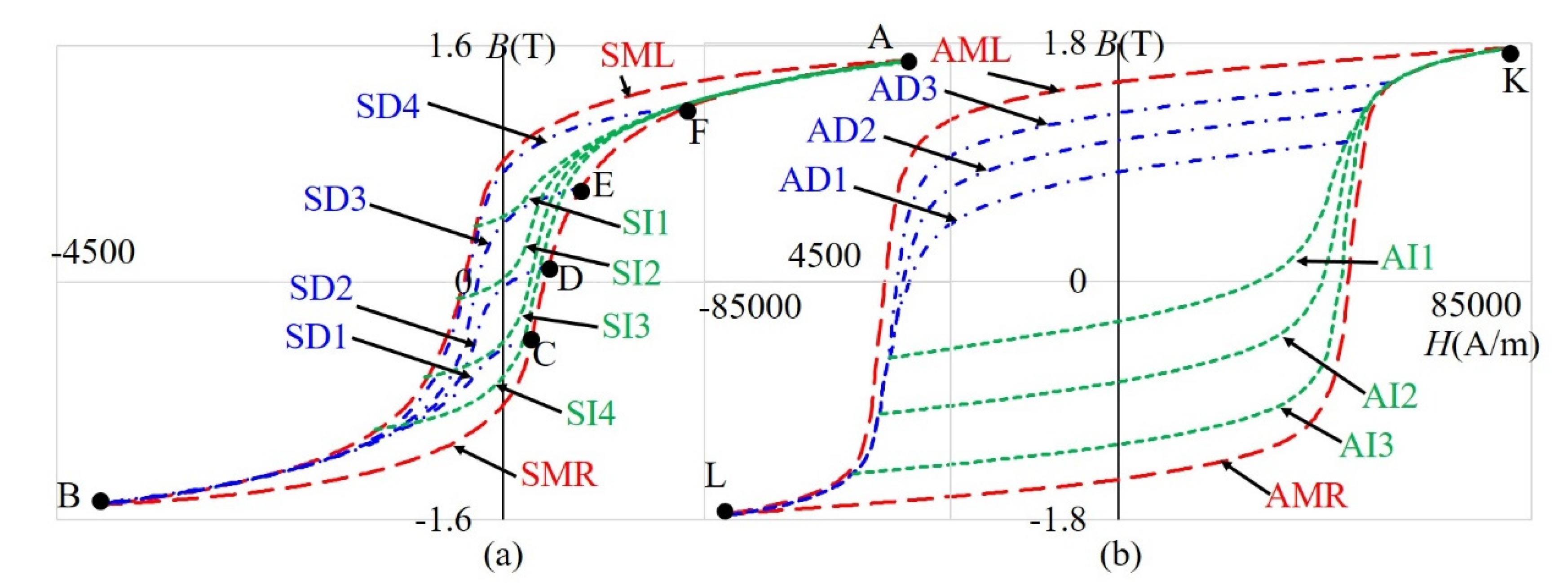
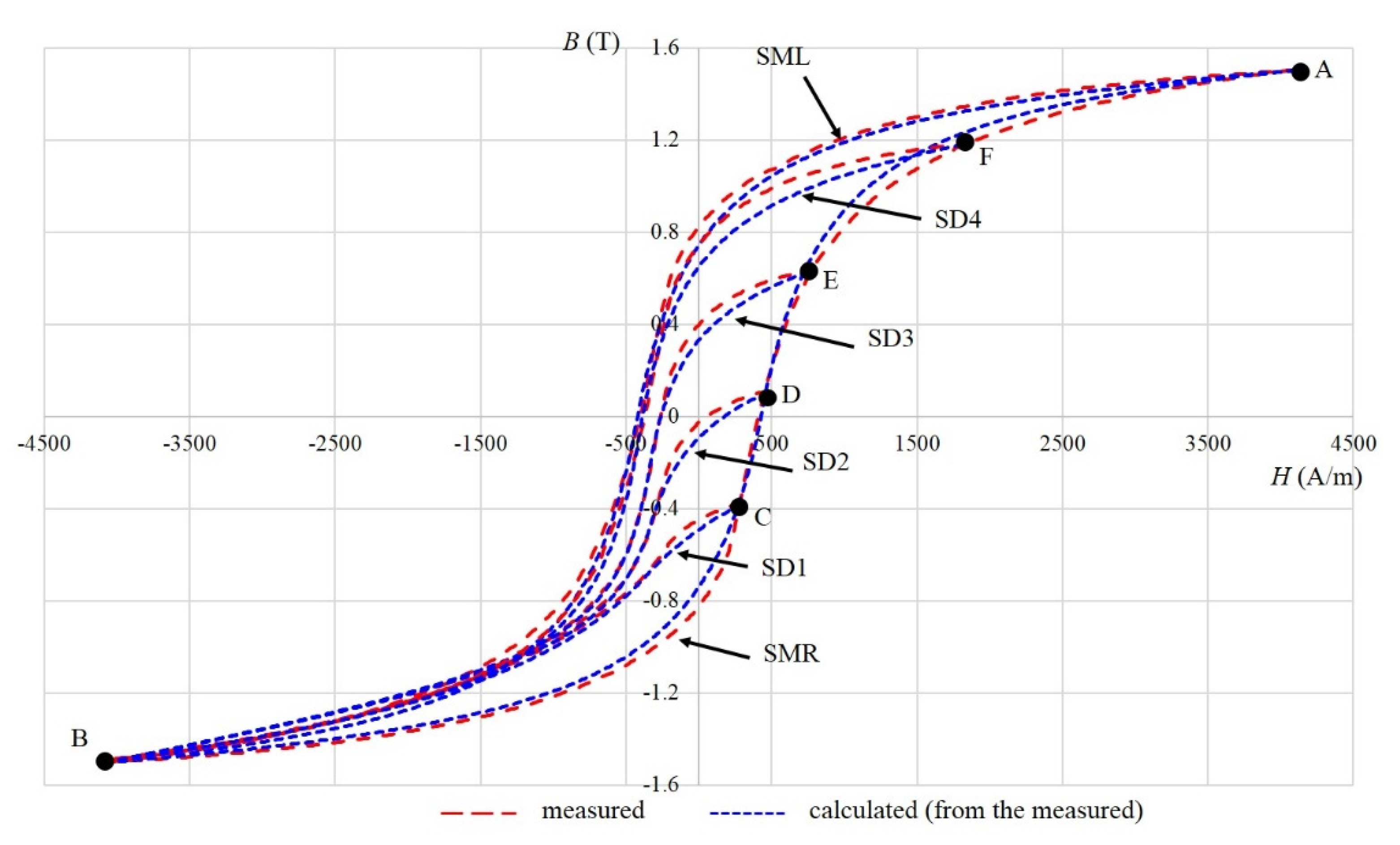
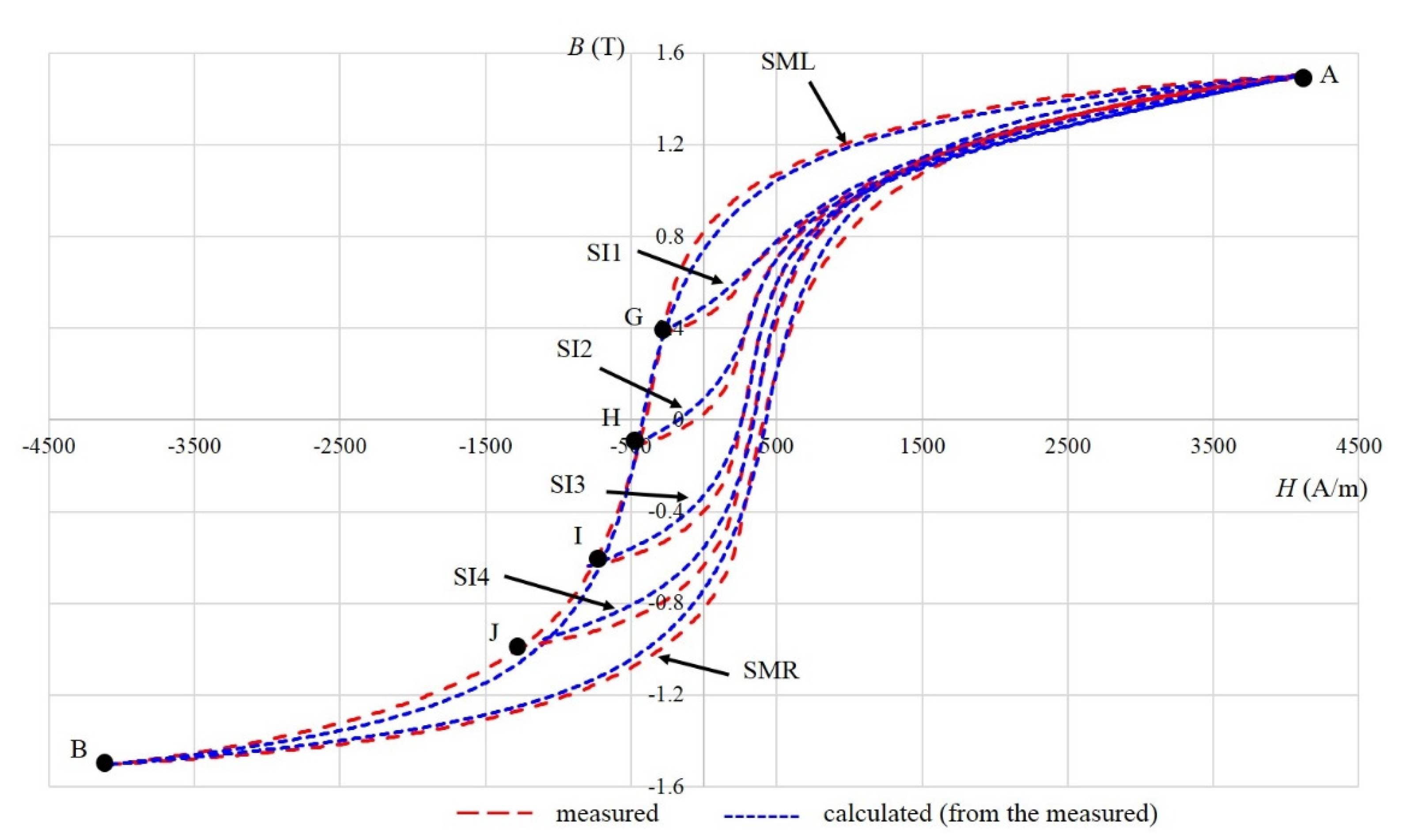
Two measured hystereses of materials 9S20 and Alnico with first-order reversal curves were used for the tests, and both are presented in Figure 2. The materials 9S20 and Alnico are magnetic, with very different hysteresis curves.

Figure 2.
Measured hysteresis of materials: (a) 9S20; (b) Alnico.
For the material 9S20, the parts of major hysteresis are marked with the left/right part of the measured major hysteresis loop (SML/SMR), decreasing first-order reversal curves are marked as SD1–SD4, and increasing first-order reversal curves are marked with SI1–SI4. For the material Alnico, the parts of major hysteresis are marked with the left/right part of the Alnico measured major hysteresis loop (AML/ AMR), decreasing curves are marked as AD1–AD3, and increasing curves are marked with AI1–AI3. The measured major hysteresis curve and first-order reversal curves were used to determine the parameters of the model. After that, only two points, the point at which the excitation is changed (for example, C–F in Figure 2) and the point at the ends of the hysteresis (for example, A and B in Figure 2), were used to determine the magnetization process in the hysteresis area between the measured curves.
No comparison between different mathematical expressions and their use on cases of very different hysteresis have been found in the literature, to know which of them is the most appropriate for the hysteresis modeling. Our contributions in this work are:
- Modification of the mathematical expressions from the literature, such as expressions from [56], by adding additional terms, with the aim to get a more suitable expression.
- Determination of a mathematical expression, selected between seven modified expressions, and determination of an appropriate method for the calculation of the parameters, selected between six methods (four methods and three different strategies of DE), to get the combination of expression and solving method which is suitable for a wide range of different materials. The appropriate method for the determination of the parameters is suggested, and tested by using it for the determination of parameters of a major hysteresis loop and more reversal curves inside the hysteresis loop for two very different materials.
- An innovative description of the magnetization process inside the hysteresis areas between the measured curves is presented, which offers a fast determination of the magnetization process and, with that, is suitable for use in the scope of the FEM calculation. It is impossible to make so many measurements that the calculation of curves in the area between the measurements would not be necessary.
Other authors have tried to make models appropriate for FEM calculation. In [7] M. Kuczmann developed an inverse vector Preisach hysteresis model, and it was inserted in the finite element procedure. Y. Zhang et al. in [57] presented a novel hysteresis core loss model for magnetic laminations, which is used in the scope of the finite element model. Like us, L. Petreswcu et al. in [56] also used Sigmoid’s functions in hysteresis phenomena modeling. The main difference between our model and other models is that, in our model, each measured curve, major and reversal, is described with different parameters, obtained using the optimization method, and the magnetization process between measured curves is described according to the nearest measured curve. In other models there is mainly only one curve, a major hysteresis or magnetization curve, used for the determination of the parameters, and all other curves are then dependent on this curve.
The paper consists of six Sections. In Section 2, different mathematical expressions are tested using standard optimization methods and evolutionary methods, and the best combination is presented of expression and method for determination of the parameters. The use of the model for the material 9S20 is presented in Section 3, and for the material Alnico in Section 4. The limits of the parameters are presented in Section 5 and the use of the model is presented in Section 6. In the last, Section 7, conclusions are given considering the proposed model.
2. Tested Mathematical Expressions and Solving Methods
Many engineering problems were solved using optimization methods. Sometimes the number of function evaluations is severely limited by time or cost. In [58] Jones et al. presented a response surface methodology to address this challenge. These surfaces can then be used for visualization, tradeoff analysis, and optimization. We were dealing with a problem presented in [59] by Jesenik et al., where the Newton–Raphson method was used to solve it. It is combined with approximation planes for a two-dimensional problem, obtained with the time consuming Finite Element Model. In the presented work, we are dealing with a curve-fitting problem, and function evaluations are not costly. Therefore, approaches for decreasing the number of fitness evaluations are not used, such as the approach with response surface methodology.
2.1. Tested Mathematical Expressions
Hysteresis occurs in various fields of engineering work [60,61,62]. In the past, different mathematical expressions were used for hysteresis modeling. The magnetization curve, and also hysteresis, can be modeled in the easiest way by using a Sigmoid function. In the literature, different expressions of the Sigmoid function can be found [56], and it plays a very important role in hysteresis modeling. A Sigmoid function is a mathematical function, which usually has an “S” shape. It is real-valued and differentiable. It is used in many fields, such as in the field of Neural Networks, to describe the processes in the human brain, in mathematical psychology, etc. We selected seven mathematical expressions of Sigmoid function from [56]. The Langevin function is related to the Boltzmann law of magnetic moment distributions. Other functions are mathematical expressions in which parameters have less physical meaning. These are used to adjust mathematical expressions to hysteresis curves.
Seven mathematical expressions from [56] are modified appropriately by adding additional terms into the expressions, and tested on the basis of two very different hystereses of a material named 9S20, with coercive magnetic field strength 4096 A/m, and a material named Alnico, with coercive magnetic field strength 47,289 A/m, and both materials are presented in Figure 2. Measurements were made in our laboratory (the Laboratory of Applied Electromagnetics at the Faculty of Electrical Engineering and Computer Science, University of Maribor). Based on our experience in working with magnetic materials, we added the following parts in each used expression:
- -
- After each H, a parameter was added in the form (H + Pa), which offers the possibility to move a curve with respect to the H axis.
- -
- Parameter + Pb was added, which offers the possibility to move a curve with respect to the B axis.
- -
- Part Pc∙μ0∙(H + Pa) was added for better adjustment of saturation.
The used modified expressions are:
Langevin:
Grompertz:
Hyptan (Hyperbolic tangents):
Algebraic:
Logistic:
Sigmoid:
Elliot:
2.2. Calculation of the Parameters Using Standard Optimization Methods
Standard optimization methods can be used for the determination of the parameters. We tested the Levenberg-Marquardt algorithm and nonlinear regression to determine their usefulness for solving the described problem.For the test of the standard optimization methods, we used Elliot’s expression (7) and SML of the material 9S20, presented in Figure 2.
The Objective Function (OF) is written in (8).
where n is the number of measured points, Bmeasured are the measured points, and Bcalculated are the calculated points.
An initial guess is needed to start standard optimization methods. The Levenberg-Marquardt (LM) algorithm is often used for solving curve-fitting problems, which is also evident from the literature [63,64]. A set of nonlinear equations was solved in the least-square sense. The minimization of a sum of squares of equation residuals was made using the LM algorithm.
Unfortunately, the local minima caused that different initial values led to different results. The lack of change of the parameters was the stopping condition of the algorithm (the maximum change must be less than 10−12). Figure 3 shows the tests for the SML curve, and the values of the parameters which were used for both the initial and final curves are presented in Table 1.
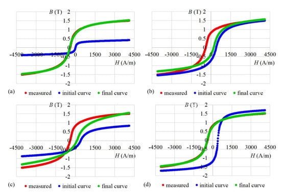
Figure 3.
Final curves obtained with Levenberg–Marquardt algorithm (LM) for curve left part of the measured major hysteresis loop (SML) using four different initial curves: (a) The correct result; (b) An incorrect result; (c) An incorrect result; (d) The correct result.

Table 1.
The OF and parameters’ values calculated with LM and used for both the initial and final analytical curves presented in Figure 3.
The results presented in Figure 3b,c are not correct (OF is 0.1548 and 0.1215). The OF for cases (a) and (d) is 6.342·10−4. Based on the results presented as (b) and (c) in Table 1 and Figure 3, it can be seen that, for two initial curves, the obtained results are in two different local minima (the final curve is not similar to the measured values), and they are not the global minimum. The results presented in (a) and (d) are global minima.
LM is very fast. A very good result can be obtained by using appropriate initial values. Due to the fact that LM is not able to bypass the local minima, it is not suitable to be used as a stand-alone method. Also, NonLinear regression using the Matlab function “nlinfit” and using analytical derivatives were not suitable for the presented problem.
2.3. Calculation of the Parameters Using Evolutionary Methods
Evolutionary optimization methods [21,22,23,24,25,26,27,28,29,30,31,32,33,34,35,36,37,38,39,40,41,42,43,44,45,46,47,48,49,50,51,52,53,54,55] are population-based search algorithms, where the space of all possible solutions is searched through many solutions with various suitability (fitness). Better solutions have a higher probability to survive into the next generation, where they might be altered by mutation and/or crossover. Evolutionary optimization methods have a remarkable ability to balance exploration and exploitation [25] and, as such, avoid local optima. They are often used for technical problems, and also to determine the parameters of different models [65] describing real material properties or real devices. In this work, we used and compared GA [21,22,23,24,25,26], DE [27,28,29,30,31,32,33,34,35,36], TLBO [37,38,39,40,41,42,43,44,45] and ABC [46,47,48,49,50,51,52,53,54,55]. In GA 0.5 was used for the fraction of the kept population, and 0.2 was used for the mutation rate. For all three used DE strategies, which were DE/rand/1/exp (Algorithm 1), DE/rand/2/exp and DE/best/1/bin, 0.8 was used for the crossover probability, and 0.6 was used for the amplification of the differential variation. Different strategies are used, because it is known that the appropriateness of the strategy depends on the problem being addressed. The duplication elimination phase was omitted in the TLBO used in our work. Therefore, the number of Fitness Evaluations (FEs) which were consumed for the calculation was determined statically as FEs = 2 * population size * iterations. The limit value used in ABC was set at 100, and was used as a control parameter for the bee population. A scout bee might not be used for every iteration [49], therefore the number of FE’s used in ABC cannot be determined statically.
| Algorithm 1. Pseudo-code for DE/rand/1/exp. |
| 1. Setting control parameters (maximum number of FEs, population size, F, Cr) |
| 2. Randomly generates the initial population of vectors in the D-dimensional search space |
| 3. repeat |
| 4. for each vector i in the population do |
| 5. select three mutually exclusive random vectors |
| 6. generate a donor vector according to (9) |
| 7. |
| 8. |
| 9. do |
| 10. |
| 11. while (rand(0,1) <= Cr AND L <= D) |
| 12. N = a random integer in the range of [1,D] |
| 13. generate a trial vector using exponential crossover by (10) |
| 14. |
| 15. evaluate the candidate vector using (8) |
| 16. replace with , if fitness of is better than fitness of |
| 17. end-for |
| 18. until a termination condition is met |
For all tests we used 83,160 FEs, which were appropriate in [66] for nine parameters, and in this work we are dealing with five (D = 5) or six parameters (D = 6). The population size is ten times the number of parameters, fifty for five parameters and sixty for six parameters. The OF which was used for the analytical curves’ quality estimation was defined previously in (8).
To compare the ability of the presented expressions (1)–(7) to express hysteresis analytically, they were tested at the left part of the 9S20 measured major hysteresis loop (SML) and AML, which are presented in Figure 2. The number of independent runs was 30 for each expression for GA, three DE strategies, (DE/rand/1/exp, DE/rand/2/exp and DE/best/1/bin), TLBO and ABC. The best (B), worst (W), mean (M) OF and standard deviation (SD) are written in Table 2 for SML, and in Table 3 for AML. In Table 2 and Table 3 the lowest best OF and the lowest mean OF are marked with bold, and the second-lowest best OF and the second-lowest mean OF are marked with italics.

Table 2.
Best (B), worst (W), mean (M) and standard deviation (SD) for 30 independent runs of different methods using expressions (1) to (7) for SML.

Table 3.
B, W, M and SD for 30 independent runs of different methods using expressions (1) to (7) for left part of the Alnico measured major hysteresis loop (AML).
For each combination of expression and method from Table 2, appropriate parameters obtained using results with the best OF are shown in Table 4. For each presented combination in Table 3, appropriate parameters obtained using results with the best OF are shown in Table 5.

Table 4.
Parameters of expressions for the results (best OF) from Table 2 for SML.

Table 5.
Parameters of expressions for the results (best OF) from Table 3 for AML.
The aim of the results presented in Table 2, Table 3, Table 4 and Table 5 is also to find out if different algorithms lead to different parameters. For Langevin, Grompertz, Hyptan and Elliot, it can be seen that, with methods that reached the same best OF, the calculated parameters are also the same. If the best OF is only a little different, the parameters are also just slightly different. In the case of algebraic, the parameters are different, although the best OF is the same. In the case of logistic and Sigmoid, the obtained best OF is different for almost every algorithm, and, consequently, the calculated parameters are also different. Although the same best OF is obtained using different methods, mean OF can be very different, which means that some methods occasionally give poor results on this problem, which is not desirable.
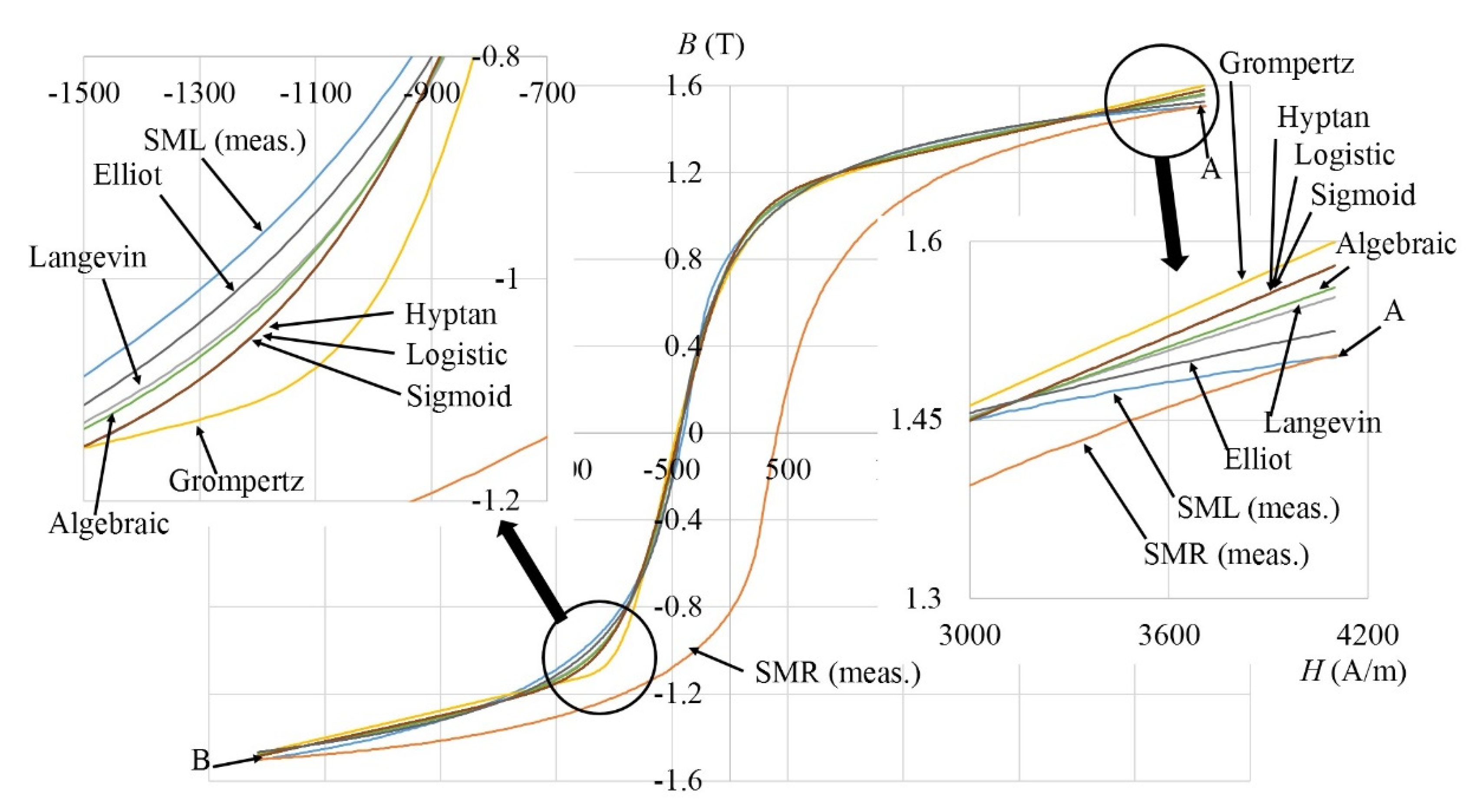
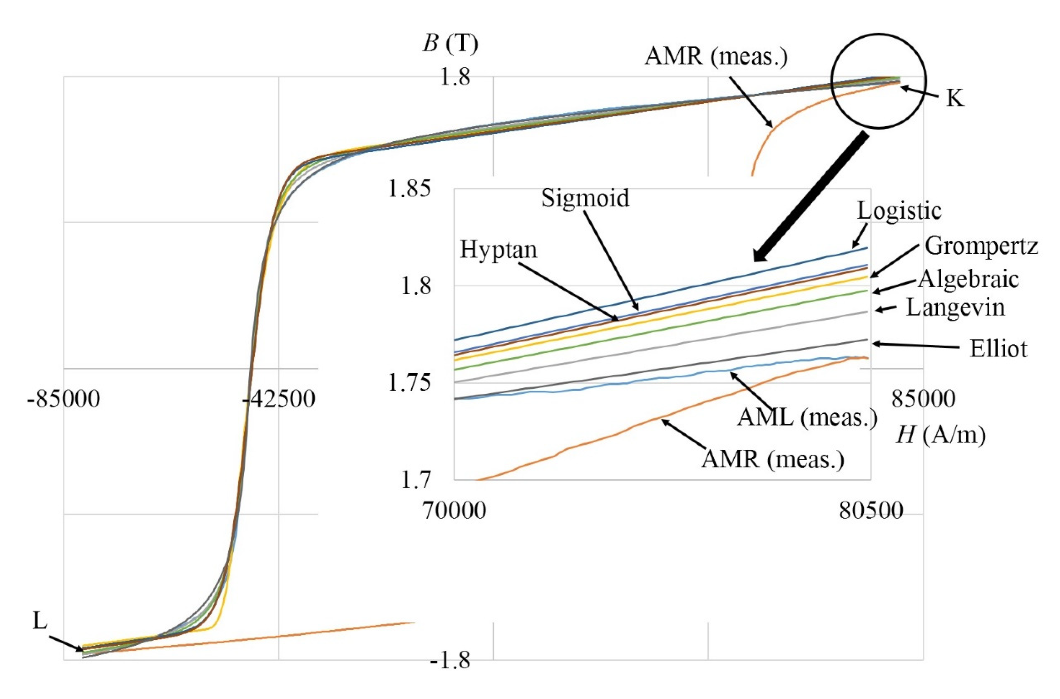
A comparison of different expressions is presented graphically in Figure 4 for SML and in Figure 5 for AML. Parameters used were obtained from the calculation with the best OF.
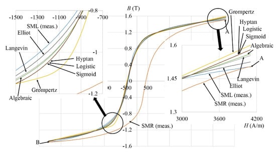
Figure 4.
Graphically presented different expressions for SML.
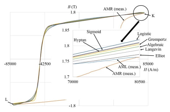
Figure 5.
Graphically presented different expressions for AML.
From Table 2 it can be seen that the best results were obtained using the Elliot expression and methods DE/rand/1/exp, DE/rand/2/exp and TLBO. The second-best result was obtained using Langevin and methods DE/rand/1/exp, DE/rand/2/exp and TLBO. On the other hand, based on Table 3, it can be observed that the best results were obtained using Langevin and methods DE/rand/1/exp and DE/rand/2/exp. The second-best result was obtained using Elliot and methods DE/rand/1/exp and DE/rand/2/exp. We can conclude that the best results were obtained using the Elliot and Langevin expressions and DE/rand/1/exp and DE/rand/2/exp solving methods. To select the best, additional tests were made based on all curves of the material 9S20 (SML, SMR, SD1–SD4, SI1–SI4) and Alnico (AML, AMR, AD1–AD3, AI1–AI3), presented in Figure 2.
In Table 6, the results of 30 independent runs are presented for all 9S20 curves from Figure 2 using DE/rand/1/exp and DE/rand/2/exp for the Elliot and Langevin expressions. In Table 7, the results of 30 independent runs are presented for all Alnico curves from Figure 2 using DE/rand/1/exp and DE/rand/2/exp for the Elliot and Langevin expressions.

Table 6.
B, W, M and SD for 30 independent runs for all 9S20 curves using DE/rand/1/exp and DE/rand/2/exp for the Elliot and Langevin expressions.

Table 7.
B, W, M and SD for 30 independent runs for all Alnico curves using DE/rand/1/exp and DE/rand/2/exp for the Elliot and Langevin expressions.
The numbers of best results achieved for the combination of expression and method presented in Table 6 and Table 7 are shown in Table 8.

Table 8.
Numbers of lowest B and M achieved using DE/rand/1/exp and DE/rand/2/exp for the Elliot and Langevin expressions.
Based on Table 8, it can be seen that the best results were obtained using a combination of the Elliot expression and DE/rand/1/exp for the determination of the parameters. Based on the presented results, we decided to use the Elliot expression, written in (7), to model the hysteresis curve, and to use DE/rand/1/exp for determination of the parameters. The meaning of parameters P1, P2 and P3 are presented in Figure 6, and the meaning of parameters P4, P5 and P6 is presented in Figure 7.

Figure 6.
Meaning of parameters: (a) P1; (b) P2; (c) P3 used in the Elliot expression.

Figure 7.
Meaning of parameters: (a) P4; (b) P5; (c) P6 used in the Elliot expression.
Parameter P3 moves the curve according to the H axis, P6 according to the B axis, and parameters P1, P2, P4 and P5 influence the shape and size of the curve.
In the continuation, the use of the Elliot expression is presented for materials 9S20 and Alnico.
2.4. Discussion of Calculated Values with Respect to Measurement Error
Measurements were made on the device for the characterization of semi and hard magnetic materials. A Magnet-Physic yoke MIR-5 was used for the measurements. A sample of massive material was made with a circular cross-section (diameter of the sample was 10 mm) was used and it was 80 mm long. A tangential Hall probe HS-TGB5-104005 with basic accuracy 0.25% (to 3T) was used for measurement of H. The Hall probe was connected with a Magnet-Physic TESLAMETER with basic accuracy 0.3% (without probe). So that the accuracy of the H measurement, considering the accuracy of the TESLAMETER and probe, was 0.55%. In the measurements we also have to consider that, between the probe which was placed fixed near the sample and the sample, a small air gap appears. The magnetic field in the cross-section of the tested material was not completely homogeneous. The real accuracy for the measurement of H was around 5%.
B was measured by induction in the measuring coil with 500 turns, coiled around the center of the sample and connected with a Fluxmeter. A Magnet-Physic Electronic Fluxmeter EF5 was used for the measurement of B. The basic accuracy of the Fluxmeter was 0.25%. The frequency of the measurement was 10 mHz. Although the measuring coil was coiled tightly around the sample, there was still some air between the coil and the sample. For the measurement of B, it should be considered that the magnetic field in the cross-section of the tested material was not completely homogeneous. Because of that, the real accuracy for the measurement of B was around 5%.
The measured and calculated values of B in point A (presented in Figure 5) for 9S20 material and point K (presented in Figure 6) for Alnico, are presented in Table 9.

Table 9.
Measured and calculated values of B at points A and K.
From Table 9 it can be seen that three calculated values at point A were inside of the measurement accuracy range, three vales were at the border, and one value was outside of the measurement accuracy range. It can also be seen that all calculated values at point K were inside of the measurement accuracy range. Points A and K are points where the deviation between the measured value and the calculation is higher, but they are important for Hysteresis modeling, as will be presented in Section 3.2 and Section 4.2. Taking into account the measurement accuracy and the results presented in Table 9, we can conclude that it is reasonable to search for expressions and methods to match the measured and calculated curves best (some calculated values were at the border or outside of the measurement accuracy range).
3. Modeling of the Material 9S20
For better understanding of the hysteresis modeling procedure, modeling is explained briefly in steps, and, after that, each step is explained in detail in the subsections. The steps are presented in Figure 8.

Figure 8.
Steps of the hysteresis modeling procedure: (a) Determination of P1 to P6 for SML; (b) Adjustment of P1 and P6 for SML; (c) Determination of analytical expressions for all measured curves; (d) Calculation of the required curves.
In step 1, presented in Figure 8a, parameters P1 to P6 are determined for the measured curve SML, based on the measured curve using Elliot’s expression and the DE/rand/1/exp method.
In step 2, presented in Figure 8b, parameters P1 and P6 are adjusted according to the appropriate points (in the case of SML, points A and B).
In step 3, presented in Figure 8c, all measured curves are replaced with analytical expressions repeating steps 1 and 2 for each measured curve.
In step 4, presented in Figure 8d, any required curve with respect to magnetization changes, as shown in Figure 1, can be calculated on the basis of two points, for example, points E1 and B.
3.1. Calculation of the Parameters Using DE/Rand/1/exp
Major hysteresis loop left and right parts (SML and SMR), first-order decreasing reversal curves (SD1–SD4) and first-order increasing reversal curves (SI1–SI4) were measured in the case of the material 9S20. The first step in the modeling procedure is to determine the Elliot expression parameters using DE/rand/1/exp. 30 independent runs were used for each measured curve. The parameters obtained with the best OF are presented in Table 10, Table 11 and Table 12. The values of B, W, M and SD were presented previously in Table 6. In Table 10, Table 11 and Table 12 parameters obtained with the best OF of the Langevin expression are also shown, in order to enable the analysis of the results.

Table 10.
Calculated parameters of the 9S20 major hysteresis loop.

Table 11.
Calculated parameters of the 9S20 decreasing first-order reversal curves.

Table 12.
Calculated parameters of the 9S20 increasing first-order reversal curves.
3.2. Adjusted Parameters P1 and P6 for 9S20
From Figure 4 it can be seen that the calculated curve SML does not flow through the hysteresis final points A and B. To adjust the calculated curve to points A and B only parameters P1 and P6 should be adjusted, using the system of two equations written in (11) and (12).
The calculated SMR first-order decreasing and increasing reversal curves also do not flow through the final points, and parameters P1 and P6 were adjusted as a result. The values of adjusted parameters are presented in Table 13, Table 14 and Table 15, where the points used for adjustment are also presented (points are shown in Figure 9 and Figure 10).

Table 13.
P1 and P6 for SML and the right part of the measured major hysteresis loop (SMR).

Table 14.
P1 and P6 for the 9S20 decreasing first-order reversal curves.

Table 15.
P1 and P6 for the 9S20 increasing first-order reversal curves.
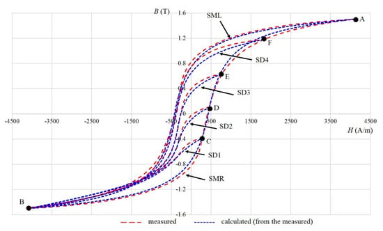
Figure 9.
Measured and calculated major hysteresis loop (SML and SMR) and first-order decreasing reversal curves (SD1–SD4).
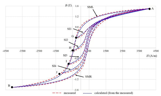
Figure 10.
Measured and calculated major hysteresis loop (SML and SMR) and first-order increasing reversal curves (SI1–SI4).
The parameters of each of the curves (decreasing and increasing), written in Table 11, Table 12, Table 14 and Table 15, were obtained using a measured curve, and, with that, they were adjusted to the form of the curve. In this way, no special adjustment is required with respect to increasing and decreasing curves. Comparing similar increasing and decreasing curves (for example SI2 and SD2, shown in Figure 2), it can be seen that parameters P1, P2, P4 and P5, which influence the shape and size, are similar. Parameter P3, which moves the curve according to the H axis, is different, and also parameter P6, which moves the curve according to the B axis, is different.
3.3. Calculation of Curves in the Area between the Measured Curves for 9S20
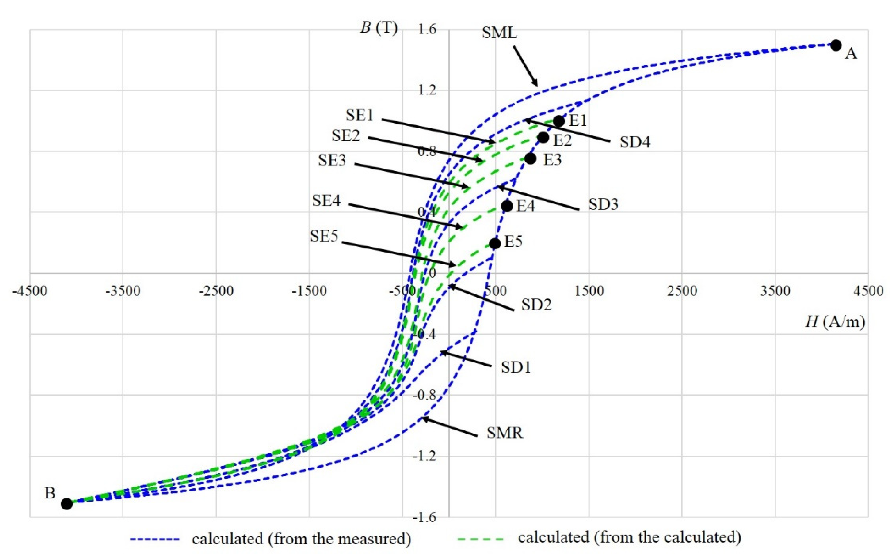
The main purpose of the presented model is to calculate the magnetization in the area between the measured curves simply. To calculate magnetization, only points where the excitation starts to decrease after increasing (for example point C marked in Figure 9 and point B marked in Figure 9) are needed to calculate the decreasing magnetization. The parameters of the nearest curve are used, obtained based on the measured curve, and parameters P1 and P6 are adjusted using a system of two equations, such as written in (11) and (12), to get the appropriate magnetization. Calculated curves are presented in Figure 11 and marked with SE1–SE5. For example, curve SE1 is calculated based on the nearest curve obtained based on measurements, which is SD4. Point E1, where the excitation starts to decrease, and point B, are used to calculate parameters P1 and P6, and parameters P2 to P5 are the same as used for the curve SD4.
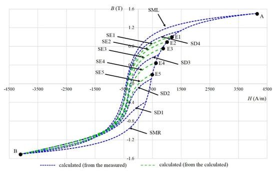
Figure 11.
Calculated curves based on the measured curves (SML, SMR, SD1–SD4) and calculated curves in the area between the measured curves SE1–SE5.
Parameters of the calculated curves SE1–SE5, together with used points and the nearest curve obtained based on the measured curve, which is the basis for the curve calculation, are presented in Table 16.

Table 16.
Parameters of the calculated curves SE1–SE5.
The same procedure can be used for increasing magnetization. The values of B and H in the points presented in Figure 9, Figure 10 and Figure 11 are determined in Table 17.
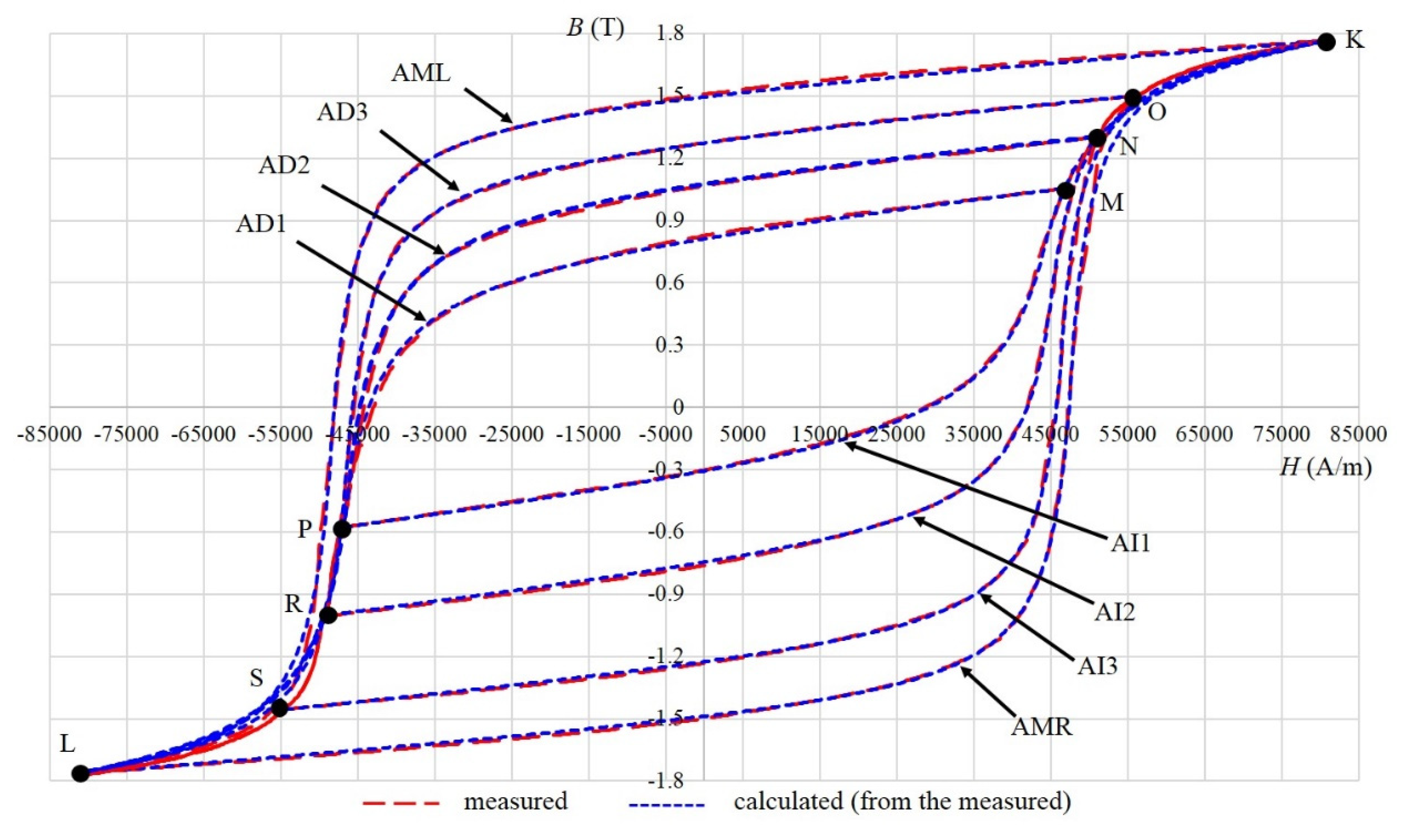
The calculated and measured major hysteresis loop, decreasing and increasing curves are presented in Figure 12.
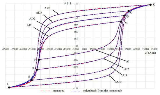
Figure 12.
Measured and calculated major hysteresis loop (AML and the right part of the Alnico measured major hysteresis loop (AMR)), decreasing curves (AD1–AD3) and increasing curves (AI1–AI3).
4. Modeling of the Material Alnico
The calculation steps of the Alnico hysteresis model are the same as presented briefly in Section 3.
4.1. Calculation of the Parameters Using DE/Rand/1/exp
A major hysteresis loop’s left and right parts (AML and AMR), decreasing curves (AD1–AD3) and increasing curves (AI1–AI3) were measured in the case of the material Alnico (presented in Figure 2). The Elliot expression parameters were determined using DE/rand/1/exp. 30 independent runs were used for each measured curve. The parameters obtained with the best OF are presented in Table 18, Table 19 and Table 20. The values of B, W, M and SD were presented previously in Table 7. In Table 18, Table 19 and Table 20 parameters obtained with the best OF of the Langevin expression are also shown in order to enable an analysis of the results.

Table 18.
Calculated parameters of the Alnico major hysteresis loop.

Table 19.
Calculated parameters of the Alnico decreasing curves.

Table 20.
Calculated parameters of the Alnico increasing curves.
4.2. Adjusted Parameters P1 and P6 for Alnico
To adjust curves to the start and end points, parameters P1 and P6 were corrected using the system of two equations, such as in (11) and (12). The values of adjusted parameters are presented in Table 21, Table 22 and Table 23, where the points used for adjustment are also presented.

Table 21.
P1 and P6 for AML and AMR.

Table 22.
P1 and P6 for the Alnico decreasing curves.

Table 23.
P1 and P6 for the Alnico increasing curves.
4.3. Calculation of Curves in the Area between the Measured Curves for Alnico
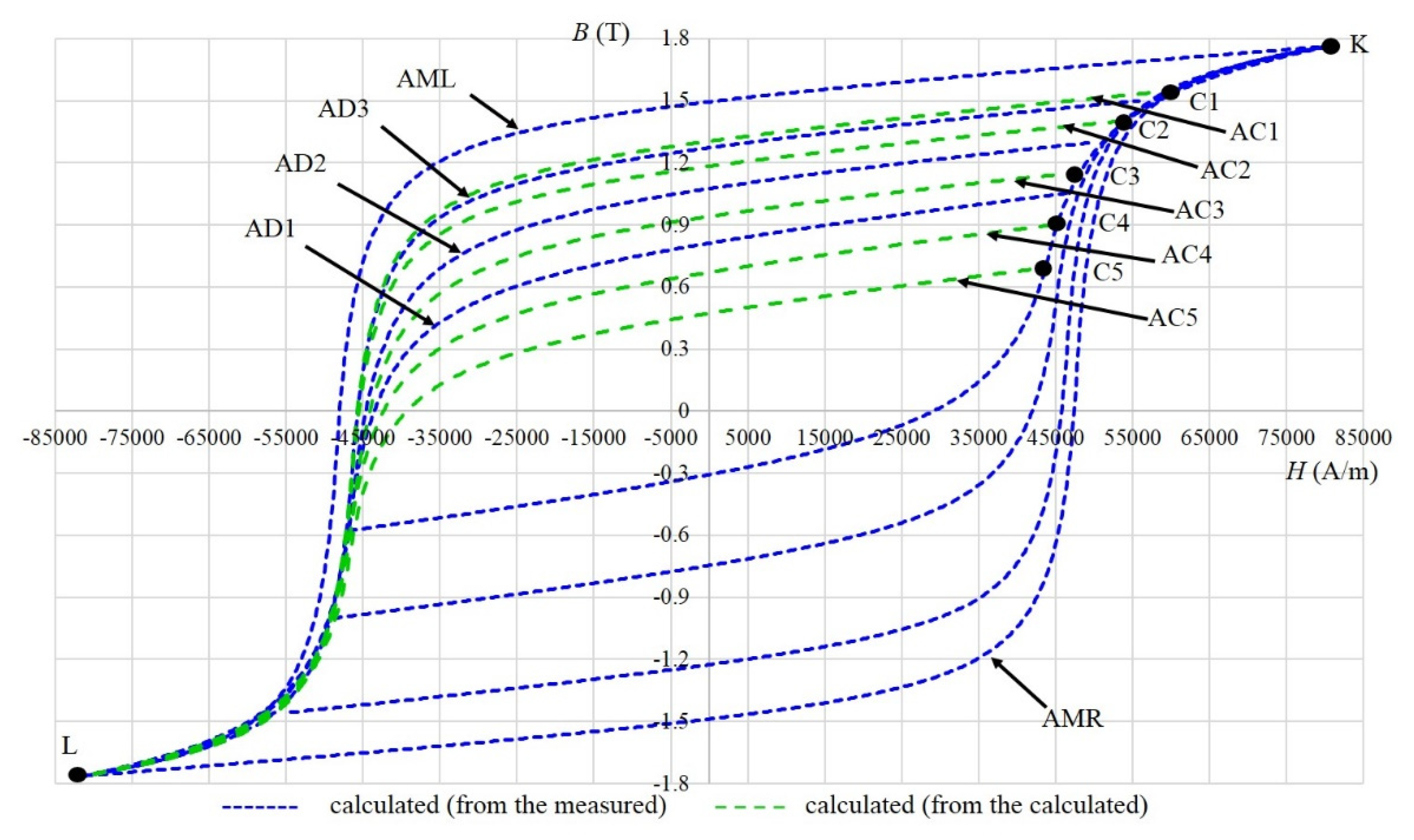
For Alnico, the curves in the areas between the calculated curves, based on measured curves, were determined using the point where the calculation started to decrease after increasing, and the point in the lower left part of the hysteresis. Calculated curves AC1–AC5 are presented in Figure 13. For example, curve AC1 was calculated based on the nearest curve obtained based on the measurement, which is AD3. Point C1, where the excitation started to decrease, and point L, were used to calculate parameters P1 and P6, using the system of two equations, such as in (11) and (12). Parameters P2 to P5 are the same as used for the curve AD3. The new magnetization curve was calculated simply, based on only two points.

Figure 13.
Calculated curves based on the measured curves (AML, AMR, AD1–AD3, AI1–AI3), and calculated curves in the area between the measured curves AC1–AC5.
The parameters of the calculated curves AC1–AC5, together with used points and the nearest curve obtained based on the measured curve, which was the basis for the curve calculation, are presented in Table 24.

Table 24.
Parameters of the calculated curves AC1–AC5.
5. Limits of the Parameters Used by Evolutionary Methods
When an evolutionary method is used, appropriate limits of the parameters should be set. Our test cases, 9S20 and Alnico, are materials with very different coercive magnetic field strength. Because of that, the limits of the parameters must contain a wide range of different values. We set limits in a way that they were appropriate for a wide range of different materials. The limits used are presented in Table 26.

Table 26.
Parameters’ limits used in the case of evolutionary calculations.
Although the limits were set wide, evolutionary methods were able to calculate parameters.
6. The Use of the Hysteresis Model
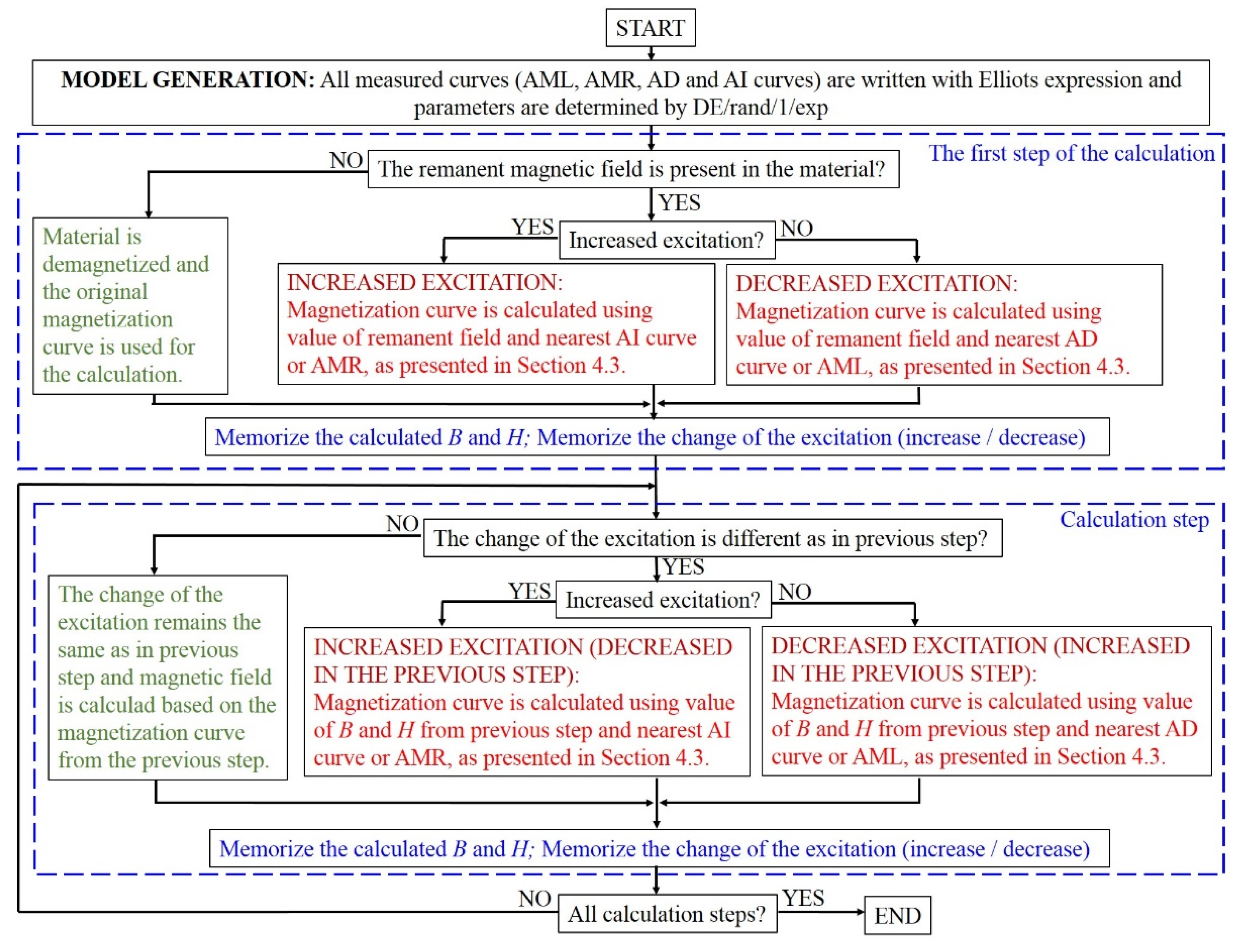
The hysteresis model is intended to be used for the transient magnetic field calculation. The algorithm presenting the use of the hysteresis model is shown in Figure 14. The curves of Alnico, presented in Figure 2, are used in the algorithm for better understanding. The basis for the model is the mathematical description of each measured curve.
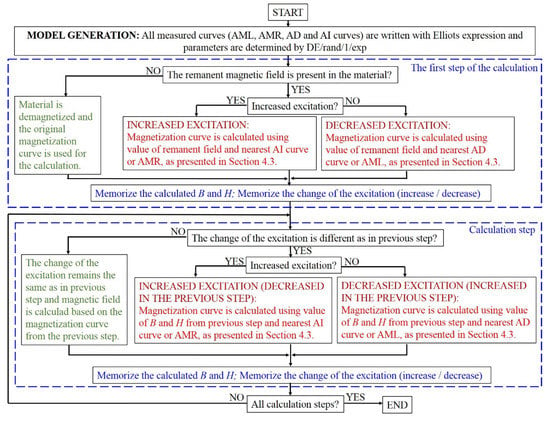
Figure 14.
Algorithm presenting the use of the hysteresis model based on Alnico curves.
Different colors are used in Figure 14 to make the algorithm more transparent. The parts of the algorithm when a new magnetization curve must be calculated are marked with red. The parts of the algorithm when the magnetization curve remains unchanged due to the previous step or an original magnetization curve is used are marked with green. The calculation depends on the excitation change, and on the calculated values of H and B from the previous step, and these data must be memorized (marked with blue color).
7. Conclusions
Precise magnetic material hysteresis modeling is important for accurate dimensioning of electromagnetic devices using FEM. The aim of the paper was to find a mathematical expression that describes a wide range of different hystereses authentically. Seven different mathematical expressions were modified appropriately with added parts, and tested on two same test examples. The results presented in Table 6, Table 7 and Table 8 show that the combination of the Elliot expression and DE/rand/1/exp method for the determination of the parameters is the best between the tested expressions and methods. Both the highest number of the lowest best OF and the highest number of the lowest mean OF were obtained using the Elliot expression combined with DE/rand/1/exp.
The idea of the model is that both major and first-order reversal measured curves could be modeled using the Elliot expression. For each measured curve, parameters were determined using DE/rand/1/exp, and, with that, the best match was achieved between measured and calculated curves. After that, a simple procedure is presented for the calculation of the curves in the area between the measured curves. Therefore, DE/rand/1/exp offers a reliable procedure for the precise determination of the parameters.
A large number of measured first-order reversal curves allow the model to function well. To simulate hysteresis, the closest curve should be selected, along with its set of six parameters. Therefore, it is impossible to simulate a curve if a similar experimental curve was not fitted previously. The model is, therefore, a fit of experimental data, and, consequently, it has no predictive ability, which is the limitation of the model.
Considering the measurement accuracy (5% for measurement of H and 5% for measurement of B) and results presented in Table 9, it can be concluded that it is reasonable to search for expressions and methods to match best the measured and calculated curves.
It can also be concluded that different algorithms lead to the same results. For almost all expressions in the case of the same calculated OF, calculated parameters are also the same. Although the same best OF is obtained using different methods, mean OF can be very different, which means that some methods occasionally give poor results on this problem, which is not desirable. Because of this, we have identified the method that is best for the presented problem.
The presented model shows the successful use of the evolutionary method for the determination of a higher number of parameters and simple determination of further magnetization processes. Findings about the used evolutionary methods, which are presented in the paper, will be used in the future to get better solutions of the optimization problems in Electromagnetics. The integration of the presented model into the FEM software will also be one of the future studies.
Author Contributions
M.J. and M.T. made the concept and methodology considering magnetics. M.M. made the methodology considering metaheuristics, and prepared guidelines for their use. M.J. developed the hysteresis model and performed calculations. M.J., M.T. and M.M. discussed the results and developed the concept of the paper. M.J. wrote the paper. M.T. reviewed and edited the paper, with emphasis on magnetics. M.M. reviewed and edited the paper with emphasis on metaheuristics. All authors have read and agreed to the published version of the manuscript.
Funding
This work was supported by the Slovenian Research Agency under Grants P2-0114 and P2-0041.
Conflicts of Interest
The authors declare no conflict of interest.
References
- Altherton, D.L.; Beattie, J.R. A Mean Field Stoner-Wohlfarth Hysteresis Model. IEEE Trans. Magn. 1990, 26, 3059–3063. [Google Scholar] [CrossRef]
- Zirka, S.E.; Moroz, Y.I.; Harrison, R.G.; Chwastek, K. On physical aspect of the Jiles-Atherton hysteresis model. Int. J. Appl. Phys. 2012, 1–4. [Google Scholar] [CrossRef]
- Du, R.; Robertson, P. Modelling of Dynamic Magnetic Hysteresis Loops and Power Losses in Laminated Steel. In Proceedings of the 17th UKM-AMSS International Conference on Modelling and Simulations, Cambridge, UK, 25–27 March 2015; pp. 432–437. [Google Scholar]
- Liu, S.T.; Huang, S.R. Using TACS Functions Within EMTP to Set Up Current-Transformer Model Based on the Jiles-Atherton Theory of Ferromagnetic Hysteresis. IEEE Trans. Power Del. 2007, 22, 2222–2227. [Google Scholar] [CrossRef]
- Preisach Memorial Book; Ivanyi, A., Ed.; Akadémiai Kiadó: Budapest, Hungary, 2005. [Google Scholar]
- Janičević, V.; Ilić, V.; Pjevalica, N.; Nikolić, M. An approach to modelling the hysteresis in ferromagnetic by adaptation of Preisach model. In Proceedings of the 22nd Telecommunications forum TELFOR, Belgrade, Serbia, 25–27 November 2014; pp. 761–764. [Google Scholar]
- Kuczmann, M. Measurement and Simulation of Vector Hysteresis Characteristics. IEEE Trans. Magn. 2009, 45, 5188–5191. [Google Scholar] [CrossRef]
- Dlala, E.; Belahcen, A.; Fonteyn, K.A.; Belkasim, M. Improving Loss Properties of the Mayergoyz Vector Hysteresis Model. IEEE Trans. Magn. 2010, 46, 918–924. [Google Scholar] [CrossRef]
- Enokizono, M. Vector Magnetic Property and magnetic Characteristic Analysis by Vector Magneto-Hysteretic E & S Model. IEEE Trans. Magn. 2009, 45, 1148–1153. [Google Scholar]
- Zeng, Z.; Udpa, L.; Udpa, S.S. Finite-Element Model for Simulation of Ferrite-Core Eddy-Current Prob. IEEE Trans. Magn. 2010, 46, 905–909. [Google Scholar] [CrossRef]
- Egea, A.C.; Almandoz, G.; Poza, J.; Ugalde, G.; Escalada, A.J. Axial-Flux-Machine Modeling With the Combination of FEM-2-D and Analytical Tools. IEEE Trans. Ind. Appl. 2012, 48, 1318–1326. [Google Scholar] [CrossRef]
- Fu, W.N.; Ho, S.L.; Zhou, P. Reduction of Computing Time for Steady-state Solutions of Magnetic Field and Circuit couple Problems Using Time-Domain Finite-Element Method. IEEE Trans. Magn. 2012, 48, 3363–3366. [Google Scholar] [CrossRef]
- Wang, G.; Wang, S.; Duan, N.; Huangfu, Y.; Zhang, H.; Xu, W.; Qiu, J. Extended Finite-Element Method for Electric Field Analysis of Insulting Plate With Crack. IEEE Trans. Magn. 2015, 51. [Google Scholar] [CrossRef]
- Trlep, M.; Hamler, A.; Jesenik, M.; Štemberger, B. The FEM-BEM Analysis of Complex Grounding Systems. IEEE Trans. Magn. 2003, 39, 1155–1158. [Google Scholar] [CrossRef]
- Brucker, F.; Vogler, C.; Feischer, M.; Praetorius, D.; Bergmair, B.; Hubner, T.; Fuger, M.; Suess, D. 3D FEM-BEM-coupling method to solve magneto static Maxwell equations. J. Magn. Magn. Mater. 2012, 324, 1862–1866. [Google Scholar] [CrossRef]
- Salas, R.A.; Pleite, J.; Olie, E.; Baarado, A. Theoretical-experimental comparison of a modelling procedure for magnetic components using finite element analysis and a circuit simulator. J. Magn. Magn. Meter. 2008, 320, 1024–1028. [Google Scholar] [CrossRef]
- Kursa, H.; Ohtake, M.; Miyagi, D.; Takahashi, N. 3-D FEM analysis of thermal degradation in writing and reading characteristics of a perpendicular magnetic head. J. Magn. Magn. Mater. 2008, 320, 2917–2920. [Google Scholar] [CrossRef]
- Zona, A.; Ranz, G. Finite element model for nonlinear analysis of steel-concrete composite beams with partial interaction in combined bending and shear. Finite Elem. Anal. Des. 2011, 47, 98–118. [Google Scholar] [CrossRef]
- Melenk, J.; Babuška, I. The partition of unity finite element method: Basic theory and applications. Comput. Methods Appl. Mech. Eng. 1996, 139, 289–314. [Google Scholar] [CrossRef]
- Hansbo, A.; Hansbo, P. A finite element method for the simulation of strong and weak discontinuities in solid mechanics. Comput. Methods Appl. Mech. Eng. 2004, 193, 3523–3540. [Google Scholar] [CrossRef]
- Goldberg, D. Genetic Algorithms in Search, Optimization and Machine Learning, 1st ed.; Addison-Wesley Longman Publishing Co.: Boston, MA, USA, 1989. [Google Scholar]
- Holland, J.H. Adaptation in Natural and Artificial Systems; The MIT Press: London, UK, 1975. [Google Scholar]
- Haupt, R.L.; Haupt, S.E. Practical Genetic Algorithms, 2nd ed.; John Wiley and Sons: Hoboken, NJ, USA, 2004. [Google Scholar]
- Cortes, P.; Larranieta, J.; Onieva, L. Genetic algorithm for controllers in elevator groups: analysis and simulation during lunchpeak traffic. Appl. Soft Comput. 2004, 4, 159–174. [Google Scholar] [CrossRef]
- Črepinšek, M.; Liu, S.H.; Mernik, M. Exploration and exploitation in evolutionary algorithms: A survey. ACM Comput. Surv. 2013, 45, Article 35. [Google Scholar]
- Haupt, R.L. Optimum population size and mutation rate for a simple real genetic algorithm that optimizes array factors. In Proceedings of the IEEE Antennas and Propagation Society International Symposium, Salt Lake City, UT, USA, 16–21 July 2000; pp. 1034–1037. [Google Scholar]
- Rocca, P.; Oliveri, G.; Massa, A. Differential Evolution as Applied to Electromagnetics. IEEE Trans. Antennas Propag. 2011, 50, 38–49. [Google Scholar] [CrossRef]
- Veček, N.; Mernik, M.; Črepinšek, M. A chess rating system for evolutionary algorithms: A new method for the comparison and ranking of evolutionary algorithms. Inf. Sci. 2014, 277, 656–679. [Google Scholar] [CrossRef]
- Mallipeddi, R.; Suganthan, P.N.; Pan, Q.K.; Tasgeriren, M.F. Differential evolution algorithm with ensemble of parameters and mutation strategies. Appl. Soft Comput. 2011, 11, 1679–1696. [Google Scholar] [CrossRef]
- Das, S.; Suganthan, P.N. Differential Evolution: A Survay of the State-of-the-Art. IEEE Trans. Evol. Comput. 2011, 15, 4–31. [Google Scholar] [CrossRef]
- Saruhan, H. Differential evolution and simulated annealing algorithms for mechanical systems design. Eng. Sci. Technol. Int. J. 2014, 17, 131–136. [Google Scholar] [CrossRef][Green Version]
- Mokan, M.; Sharma, K.; Sharma, H.; Verma, C. Gbest guided differential evolution. In Proceedings of the 9th International Conference on Industrial and Information Systems, Gwalior, India, 15–17 December 2014; pp. 1–6. [Google Scholar]
- Chattopadhyay, S.; Sanyal, S.K.; Chandra, A. Optimization of Control Parameters of Differential Evolution Technique for the Design of FIR Pulse-shaping Filter in QPSK Modulated System. J. Commun. 2011, 6, 558–570. [Google Scholar] [CrossRef][Green Version]
- He, R.-J.; Yang, Z.-Y. Differential Evolution with Adaptive Mutation and Parameter Control Using Lévy Probability Distribution. J. Comput. Sci. Technol. 2012, 27, 1035–1055. [Google Scholar] [CrossRef]
- Reed, H.M.; Nichols, J.M.; Earls, C.J. A modified differential evolution algorithm for damage identification in submerged shell structures. Mech. Syst. Signal Pr. 2013, 39, 396–408. [Google Scholar] [CrossRef]
- Mohamed, A.W.; Sabry, H.Z.; Abd-Elaziz, T. Real parameter optimization by an effective differential evolution algorithm. Egypt. Inform. J. 2013, 14, 37–53. [Google Scholar] [CrossRef]
- Rao, R.V.; Savsani, V.J.; Vakharia, D.P. Teaching-learning-based optimization: A novel method for constrained mechanical design optimization problems. Comput. Aided Des. 2011, 43, 303–315. [Google Scholar] [CrossRef]
- Rao, R.V.; Savsani, V.J.; Vakharia, D.P. Teaching-Learning-Based Optimization: An optimization method for continuous non-linear large scale problems. Inf. Sci. 2012, 183, 1–15. [Google Scholar] [CrossRef]
- Rao, R.V.; Patel, V. An elitist teaching-learning-based optimization algorithm for solving complex constrained optimization problems. Int. J. Ind. Eng. Comput. 2012, 3, 535–560. [Google Scholar] [CrossRef]
- Črepinšek, M.; Liu, S.H.; Mernik, L. A note on leaching-learning-based optimization algorithm. Int. Sci. 2012, 212, 79–93. [Google Scholar]
- Waghmare, G. Comments on “A note on teachnig-learning-based optimization algorithm”. Inf. Sci. 2013, 229, 159–169. [Google Scholar] [CrossRef]
- Črepinšek, M.; Liu, S.H.; Mernik, L.; Mernik, M. Is a comparison of results meaningful from the inexact replications of computational experiments. Soft Comp. 2016, 20, 223–235. [Google Scholar] [CrossRef]
- Baghlani, A.; Makiabadi, M.H. Teaching-learning based optimization algorithm for shape and size optimization of truss structures with dynamic frequency constraints. IJST Trans. Civ. Eng. 2013, 37, 409–421. [Google Scholar]
- Sahu, B.K.; Pati, S.; Mohanty, P.K.; Panda, S. Teaching–learning based optimization algorithm based fuzzy-PID controller for automatic generation control of multi-area power system. Appl. Soft Comput. 2015, 27, 240–249. [Google Scholar] [CrossRef]
- Pickard, J.; Carretero, J.; Bhavsar, V. On the convergence and origin bias of the Teaching-Learning-Based-Optimization algorithm. Appl. Soft Comput. 2016, 46, 115–127. [Google Scholar] [CrossRef]
- Karaboga, D.; Basturk, B. A powerful and efficient algorithm for numerical function optimization: Artificial bee colony (ABC) algorithm. J. Glob. Optim. 2007, 39, 459–471. [Google Scholar] [CrossRef]
- Karaboga, D.; Basturk, B. On the performance of artificial bee colony (ABC) algorithm. Appl. Soft Comput. 2008, 8, 687–697. [Google Scholar] [CrossRef]
- Karaboga, B.; Akay, B. A Comparative Study of Artificial Bee Colony Algorithm. Appl. Math. Comput. 2009, 214, 108–132. [Google Scholar] [CrossRef]
- Mernik, M.; Liu, S.H.; Karaboga, D.; Črepinšek, M. On clarifying misconceptions when comparing variants of the Artificial Bee Colony Algorithm by offering a new implementation. Inf. Sci. 2015, 291, 115–127. [Google Scholar] [CrossRef]
- Ozturk, C.; Karaboga, D. A novel clustering approach: Artificial Bee Colony (ABC) algorithm. Appl. Soft Comput. 2011, 11, 652–657. [Google Scholar]
- Kiran, M.S.; Gündüz, M. The Analysis of Peculiar Control Parameters of Artificial Bee Colony Algorithm on the Numerical Optimization Problems. J. Comput. Commun. 2014, 2, 127–136. [Google Scholar] [CrossRef]
- Yan, G.; Li, C. An Effective Refinement Artificial Bee Colony Optimization Algorithm Based on Chaotic Search and Application for PID Control Tuning. J. Comput. Inf. Syst. 2011, 7, 3309–3316. [Google Scholar]
- Özyon, S.; Aydin, D. Incremental artificial bee colony with local search to economic dispatch problems with ramp rate limits and prohibited operating zones. Energy Convers. Manag. 2013, 65, 397–407. [Google Scholar] [CrossRef]
- Jing, B.; Hong, L. Improved Artificial Bee Colony Algorithm and Application in Path Planning of Crowd Animation. Int. J. Control Autom. 2015, 8, 53–66. [Google Scholar] [CrossRef]
- Dwivedl, A.K.; Ghosh, S.; Londhe, N.D. Modified artificial bee colony optimisation based FIR filter design with experimental validation using field-programmable gate array. IET Signal Process. 2016, 10, 955–964. [Google Scholar] [CrossRef]
- Petrescu, L.; Cazacu, E.; Petrescu, C. Sigmoid Functions Used in Hysteresis Phenomenon Modeling. In Proceedings of the 9th International Symposium on Advanced Topics in Electrical Engineering, Bucharest, Romania, 7–9 May 2015; pp. 521–524. [Google Scholar]
- Zhang, Y.; Cheng, M.C.; Pillay, P. A Novel Hysteresis Core Loss Model for Magnetic Laminations. IEEE Trans. Energy Convers. 2011, 26, 993–999. [Google Scholar] [CrossRef]
- Jones, R.D.; Schonlau, M.; Welch, W. Efficient Global Optimization Expensive Black-Box Functions. J. Glob. Optim. 1998, 13, 455–492. [Google Scholar] [CrossRef]
- Jesenik, M.; Goričan, V.; Trlep, M. Characterisation of crack’s dimensions using eddy current field measurement. Nondestruct. Test. Eval. 2013, 28, 181–193. [Google Scholar] [CrossRef]
- An, D.; Li, H.; Xu, Y.; Zhang, L. Compensation of Hysteresis on Piezoelectric Actuators Based on Tripartite PI Model. Micromachines 2018, 9, 44. [Google Scholar] [CrossRef]
- Zou, J.; Gu, G. Modeling the Viscoelastic Hysteresis of Dielectric Elastomer Actuators with a Modified Rate-Dependent Prandtl-Ishlinskii Model. Polymers 2018, 10, 525. [Google Scholar] [CrossRef]
- Qin, Y.; Zhao, X.; Zhou, L. Modeling and Identification of the Rate-Dependent Hysteresis of Piezoelectric Actuator Using a Modified Prandtl-Ishlinskii Model. Micromachines 2017, 8, 114. [Google Scholar] [CrossRef]
- Fan, J. A modified Levenberg-Marquardt algorithm for singular system of nonlinear equations. J. Comput. Math. 2003, 21, 625–636. [Google Scholar]
- Ho, H.W.; Wong, S.C. A Levenberg-Marquardt iterative solver for least-squares problems. Commun. Numer. Methods Eng. 2005, 21, 327–335. [Google Scholar] [CrossRef]
- Liu, S.-H.; Mernik, M.; Hrncic, D.; Črepinšek, M. A parameter control method of evolutionary algorithms using exploration and exploitation measures with a practical application for fitting Sovova’s mass transfer model. Appl. Soft Comput. 2013, 13, 3792–3805. [Google Scholar] [CrossRef]
- Jesenik, M.; Beković, M.; Hamler, A.; Trlep, M. Analytical modelling of a magnetization curve obtained by the measurements of magnetic materials’ properties using evolutionary algorithms. Appl. Soft Comput. 2017, 52, 387–408. [Google Scholar] [CrossRef]
© 2020 by the authors. Licensee MDPI, Basel, Switzerland. This article is an open access article distributed under the terms and conditions of the Creative Commons Attribution (CC BY) license (http://creativecommons.org/licenses/by/4.0/).

