Attraction Basins in Metaheuristics: A Systematic Mapping Study

Abstract

Context: In this study, we report on a Systematic Mapping Study (SMS) for attraction basins in the domain of metaheuristics. Objective: To identify research trends, potential issues, and proposed solutions on attraction basins in the field of metaheuristics. Research goals were inspired by the previous paper, published in 2021, where attraction basins were used to measure exploration and exploitation. Method: We conducted the SMS in the following steps: Defining research questions, conducting the search in the ISI Web of Science and Scopus databases, full-text screening, iterative forward and backward snowballing (with ongoing full-text screening), classifying, and data extraction. Results: Attraction basins within discrete domains are understood far better than those within continuous domains. Attraction basins on dynamic problems have hardly been investigated. Multi-objective problems are investigated poorly in both domains, although slightly more often within a continuous domain. There is a lack of parallel and scalable algorithms to compute attraction basins and a general framework that would unite all different definitions/implementations used for attraction basins. Conclusions: Findings regarding attraction basins in the field of metaheuristics reveal that the concept alone is poorly exploited, as well as identify open issues where researchers may improve their research.

1. Introduction

The concept of attraction basins has been used in many fields, such as Economy [1,2,3], Mathematics [4,5,6], Biology [7,8,9], Physics [10,11,12], Computer Science [13,14,15], etc. Their definitions may vary in different degrees (even within the same field), although the underlying idea stays the same. For example, to analyse far-sighted network formation games in Economy, Page et al. [2] define attraction basin informally as “… a set of equivalent networks to which the strategic network formation process represented by the game might tend and from which there is no escape”. To analyse the dynamical behaviour of different Steffensen-type methods in Applied Mathematics, Cordero et al. [5] define attraction basins as follows: “If a fixed point p of R is attracting, then all nearby points of p are attracted toward p under the action of R, in the sense that their iterates under R converge to p. The collection of all points whose iterates under R converge to p is called the basin of attraction of p.” To study the environmental robustness of biological complex networks, Demongeot et al. [7] describe an attraction basin as “the set of configurations that evolve towards an attractor …”. Similarly, in Physics, Isomäki et al. [10] describe attraction basins as “the sets of initial conditions approaching particular attractors when time approaches infinity”. In this paper, we are interested in attraction basins used in the field of Computer Science related to metaheuristics [16]. Informally, the common general definition may be stated as follows. The attraction basin consists of initial configurations that are “attracted” to its attractor. The definition allows arbitrary configurations, an arbitrary attraction mechanism, and arbitrary attractor, as long as it is reachable by the attraction mechanism from the initial configuration(s). The concept of attraction basins helps the users to structure the space under consideration, and, thus, it is applicable to almost any field.

In the field of metaheuristics, the space under consideration is composed of many feasible solutions (configurations) to the optimisation problem. Then, the metaheuristics, such as Evolutionary Algorithms,  [17,18,19,20] are used to find the (sub-)optimal solution(s). The definition of optimality depends on the needs of a concrete user. During the run, the metaheuristic itself structures the problem space to find the (sub-)optimal solution(s). This structuring depends on the internal mechanisms of a metaheuristic, user-defined parameters (if they exist), and the problem to be solved. Therefore, each metaheuristic (with all its user-defined parameters) solving some problem can be analysed with its own attraction basins [14]. However, as these attraction basins would be stochastic and hard to analyse, researchers mostly do not use metaheuristics for their construction. Researchers rely on a deterministic local search algorithm, usually Best or First Improvement, that operates on some predefined neighbourhood. In this way, each optimisation problem has its attraction basins independent of the metaheuristics used to solve it. 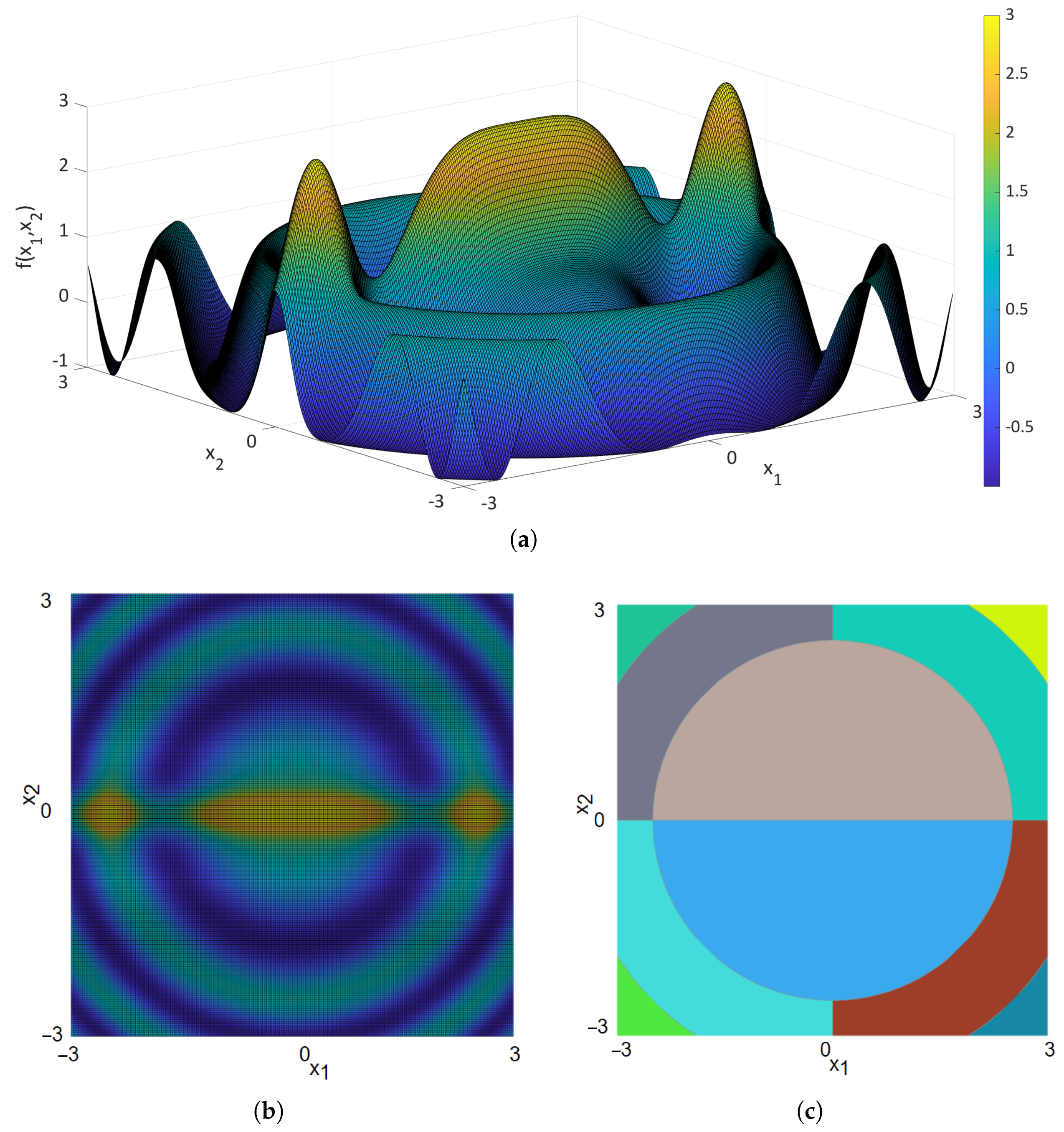For example, see Figure 1, where a landscape (Figure 1a), heatmap (Figure 1b), and attraction basins (Figure 1c) are shown for a two-dimensional Rastrigin function (see Equation (1)).

$$f(x_1\cdots x_D)=10D+\sum _{i=1}^D(x_i^2-10cos\left(2\pi x_i\right)),-5.12\le x_i\le 5.12$$

(1)

In Figure 1c, the neighbouring points (i.e., solutions and configurations) that belong to the same attraction basin have the same colour, and all points in a particular attraction basin are attracted by the same local optimum. Colours are chosen randomly, however different colour combination classes may have some impact on noticeability in map-based information visualisation as found in [21]. Here, the attraction basins were computed by a Best Improvement local search that operated on eight neighbours per each point (we used grid sampling). Attraction basins for Split Drop Wave (see Equation (2)) are not so simple and regular as for the Rastrigin function. Its attraction basins are harder to compute with the previous algorithm, due to thin circular plateaus.

$$f(x_1,x_2)=cos(x_1^2+x_2^2)+2\ast e^{-10\ast x_2^2},-3\le x_1,x_2\le 3$$

(2)

Figure 2 presents a landscape, heatmap, and attraction basins computed correctly with the algorithm from [22].

Attraction basins are used, for example, to characterise the fitness landscapes (see, e.g., in [23,24]), or analyse the metaheuristic (e.g., researchers in [22,25] measure exploration). A fitness landscape is an important concept, which was borrowed from biology [26] to analyse the optimisation problems and the relation of their characteristics to the performance of metaheuristics [27,28,29,30]. For example, characteristics such as the modality, distribution of attraction basin sizes, global and largest attraction basin ratio, global and largest attraction basin distance, barriers (optimal fitness value needed to reach one optimum from another using an arbitrary path [29]), ruggedness, etc. were compared with the performance of metaheuristics, to find out which metaheuristic was more suitable for certain characteristics of problems [31,32,33,34]. Moreover, Machine Learning algorithms were used for automatic selection of metaheuristics based on these characteristics [35,36]. Therefore, the characteristics (e.g., attraction basins) should be computed and understood accurately, otherwise such analysis could be misleading. The same holds for the exploration and exploitation, two distinct phases of each metaheuristic that are found to be crucial to understand and use metaheuristics efficiently [37,38,39,40,41]. 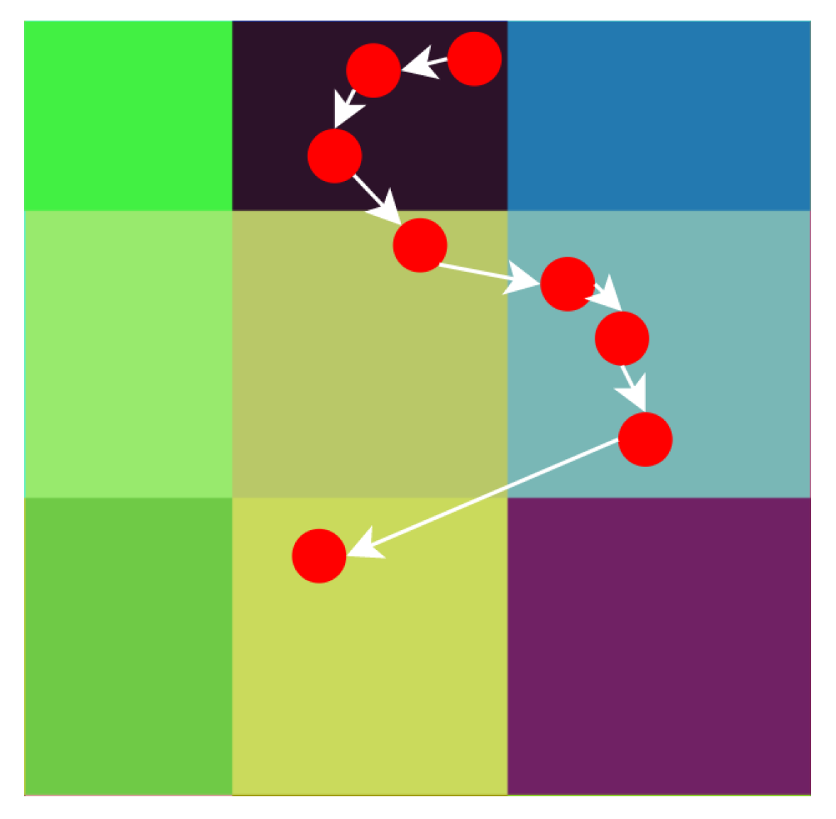In [22], attraction basins were used to measure exploration and exploitation directly. For example, in Figure 3, attraction basins are denoted with different colours, solutions given by a certain metaheuristic are denoted with red circles, and the sequence of solutions is ordered by the white arrows. The first two arrows represent the exploitation phase. The next two arrows represent the exploration phase. Then two arrows represent the exploitation phase again, and, finally, the last arrow represents the exploration phase.

It is obvious that the metric requires unambiguously computed attraction basins, so the exploration and exploitation phases can also be identified unambiguously. Otherwise, the results of the metric may be meaningless.

During our previous work, where we measured the exploration and exploitation of metaheuristics based on attraction basins [22], we noticed the inconsistencies in the definitions, lack of implementations, and generally the lack of literature that deals appropriately with the attraction basins in the field of metaheuristics, especially within continuous (real-valued domain) problems. To overcome this, we decided to conduct a Systematic Mapping Study (SMS) [42]. To the best of our knowledge, no SMS, or Systematic Literature Review (SLR) for that matter, exists on this topic in the field. We believe this study could provide a good start and point out open issues to the newcomers, as well as experienced researchers. The main contributions of this work are overviews of

• optimisation problem types where attraction basins have been used,
• topics and contexts within attraction basins have been used,
• definitions of attraction basins,
• algorithms to compute attraction basins, and
• trends.

The rest of the paper is organised as follows. Section 2 reviews SMSs and metaheuristics briefly in general. The research method is described in Section 3. Results are aggregated and discussed in Section 4. Findings are summarised and some directions are provided in Section 5. Finally, algorithms that are of secondary importance are included in Appendix A.

2. Related Work

2.1. Systematic Review

Primary studies provide original records of some research, while secondary studies aim to synthesise information about primary studies. A secondary study conducted on the secondary studies is known as a tertiary study. If a secondary study is done in a systematic manner, it is often called a Systematic Review (SR) in a broader sense. However, this term is sometimes used as a synonym for SLR. For example, Petersen et al. use SR interchangeably with SLR [43], while Kosar et al. consider SR as a higher-order category that includes SMS and SLR [44]. Evidence-based secondary studies in Software Engineering were popularised in the early 2000s by Kitchenham, Dyba, and Jorgensen borrowing the methodology from medical sciences [42,45,46,47]. These studies aim to identify all relevant evidence on the topic/area or research question. Up to now, many such studies were published in Computer Science journals or conferences [48,49,50,51]. They are found to be useful for educational purposes as well, providing a good starting point for a PhD work [52]. This was also confirmed more recently by Felizardo K. R. et al. in [53]. Generally, two types of studies, either secondary or tertiary, are distinguished:

• A Systematic Literature Review: Very specific research goals with emphasis on quality assessment, usually done by experienced researchers, closely defined by research questions [54].
• A Systematic Mapping Study: Usually broader research goals to discover research trends without any quality assessment, can be done by inexperienced researchers as well, defined by topic area [43,54].

Although a rigorous methodology is needed for an SMS as well, Wohlin et al. found that two studies performed by two independent groups addressing the same topic had a number of differences [55]. Adding to this classification by inexperienced researchers, the problem of replication, the usability of SMSs has been questioned [44]. By contrast, the authors of [56] introduced the method of random sampling and margin of error, thus reducing the amount of effort, and obtained similar results as before when they examined each study. It seems that it is a problem specific question whether to use as many publications as possible, or some subset. Initially, in SMSs database searches were conducted to aggregate studies, although, Wohlin later provided guidelines for snowballing [57]. In these guidelines, Wohlin introduces backward snowballing and forward snowballing as a new approach to gather publications, where “backward snowballing means using the reference list to identify new papers to include” and “forward snowballing refers to identifying new papers based on those papers citing the paper being examined” [57]. This procedure requires a starting set of papers, the so-called seed. A seed can be formed by a database search or by some experienced researcher. Once a seed set is formed, Mourão proposes the different snowballing procedures [58] presented in Figure 4. The first one is called iterative snowballing, because it is performed exhaustively. This means forward and backward snowballing is conducted on the papers obtained by forward and backward snowballing until no new papers are found [57,58] (Figure 4a). Parallel snowballing means papers obtained by forward snowballing are not subject to backward snowballing, and vice versa [58] (Figure 4b). Sequential backward and forward snowballing denotes the procedure where forward snowballing is run only after finishing all iterations of backward snowballing [58] (Figure 4c). Last, sequential forward and backward snowballing means the backward snowballing is run only after finishing all iterations of forward snowballing [58] (Figure 4d). Dieste O. et al. in [59] define precision and recall as follows: “A search’s sensitivity is its ability to identify all of the relevant material. On the other hand, precision is the amount of relevant material there is among the material retrieved by the search.” Recently, Mourão et al. compared the performance of different hybrid strategies that include snowballing and found out that a combination of database searches from the Scopus database with parallel or sequential snowballing achieved the most appropriate balance of precision and recall [58]. Nevertheless, strong claims about a good searching strategy should be tested in different (sub)fields and with different research questions.

Due to the increasing number of SMSs and SLRs, guidelines and methodology are being updated. However, the most commonly applied guidelines are still from Kitchenham and Charters [60] and Petersen et al. [43,61]. Recently, the emphasis has been on speeding up the screening process when performing SR [62]. Some SLRs and SMSs are conducted including grey literature beside published academic (formal) literature, a so-called Multivocal Literature Review (MLR), with their own guidelines [63]. Examples of grey literature are, e.g., presentations, videos, news articles, blogs, tweets, websites, emails, and so on. Kamei et al. propose using different shades of grey to categorise them [64]. Recently, there have been concerns about performing guidelines updates frequently, and it is reasoned that updates should be made only if necessary and with a good justification [65].

2.2. Metaheuristics

Metaheuristics are approximate methods used mainly for solving so-called intractable problems, problems that are not solvable by a polynomial-time algorithm [66]. They are found to be successful on many difficult combinatorial and/or real-valued problems. The problem space is enormously big [67,68]; thus, a good metaheuristic should navigate through the space intelligently, that is, spend as few resources as possible to find good enough solutions. To develop these metaheuristics, researchers usually find use of some phenomena observed from nature. For example, it has been observed that when an ant goes from a nest to a food source it deposits pheromones. Consequently, on shorter paths ants leave more pheromones than on longer ones. Therefore, paths with higher concentrations of pheromones are more likely to be chosen by ants. This behaviour increases the efficiency of ants while seeking food. This observation helped researchers to develop the Ant Colony Optimisation algorithm for travelling salesman problems, as ants and salesmen share the same goal, seeking the shortest path [69,70]. Similarly, researchers incorporated the concept of evolution into the widely used group of metaheuristics, the so-called Evolutionary Algorithms, that model genetic inheritance and natural selection [71]. Nowadays, there are at least one-thousand metaheuristics, and the problem of the development of metaheuristics is replaced by the problem of the analysis of metaheuristics. This is due to the proof that no single metaheuristic outperforms all other metaheuristics on all possible problems (the no free lunch theorem) [72]. Researchers in [73] found out that some state-of-the-art metaheuristics that outperform all other metaheuristics on a set of benchmark functions perform surprisingly poorly on real-world problems. Therefore, the question becomes which metaheuristic will perform sufficiently well on the set of real-world problems (this is only a subset of the set of all possible problems). To tackle this question, different approaches were used; although, for this work, the relevant ones are those that make use of attraction basins. In this respect, the most popular approach is based on Fitness Landscape Analysis [74]. For example, the number of attraction basins, distribution of their sizes, ratios of the global attraction basin and the biggest local attraction basin, and the centrality of optima have been used as indicators of problem difficulty (see, e.g., in [11,23,24,75]). Attraction basins were used as features for automated algorithm selection as well [35]. Recently, attraction basins have received some attention for delineation of the exploration and exploitation phase [22,25,76,77]. This topic is found to be one of the key topics in the field of metaheuristics [37,39]. Due to the wide presence of attraction basins in the field, and its importance on the analysis of exploration and exploitation, this SMS is an indispensable step towards a better understanding of metaheuristics.

3. Method

In this work, we used guidelines similar to those presented by Kitchenham in [60], Petersen et al. in [61], and Wohlin in [55]. Besides the usual database search, we decided to use iterative snowballing to gather as many publications as possible, because, in the preliminary search we found that the evidence on the topic is limited. In general, our study consists of the following phases:

• Defining research questions.
• Conducting a search for studies (constructing a seed set).
• Full-text screening based on inclusion/exclusion criteria.
• Iterative snowballing (each study is full-text screened prior to the next iteration).
• Classifying the studies.
• Data extraction and aggregation.

3.1. Research Questions

The main goal of this study was to obtain a first brief overview of research on attraction basins in the field of metaheuristics in the form of SMS. An SMS requires a set of research questions that mark the goals more precisely. Therefore, we set six main research questions related to metaheuristics:

• RQ1: What terms (synonyms) have been used for attraction basins?
• RQ2: For which problem types (discrete, real-valued, static, dynamic, single-objective, and multi-objective) have attraction basins been used? Which search spaces are investigated on the topic better?
• RQ3: Which definitions have been used for attraction basins?
• RQ4: Which algorithms have been developed to compute attraction basins?
• RQ5: For what topics have attraction basins been used? What is the most popular topic?
• RQ6: Which journals and conferences publish the papers on the topic, and how often? Which authors investigate attraction basins more in-depth and which type of problems?

3.2. Search, Screening Criteria, and Classification

To conduct a search, first, it is important to decide on the inclusion/exclusion criteria. To include a study we check if

• the study is in the field of Computer Science and related to metaheuristics,
• the study deals with attraction basins, and
• the study is published in a journal or conference.

To exclude the study we used the following criteria:

• The study is not presented in English.
• The study is not in a final publication stage.
• The study is not accessible in full-text.
• The study is a duplicate of another study.
• The study only mentions attraction basins without any further elaboration.

It is obvious that the last exclusion criteria can be used only after a full-text read. Therefore, full-text screening needs to be performed prior to any snowballing. We used two popular databases to form a seed set: ISI Web of Science (https://www.webofscience.com/wos/alldb/advanced-search, accessed on 25 May 2021) and Scopus (https://www.scopus.com/search/form.uri?display=advanced, accessed on 26 May 2021). The search strings are formulated as follows:

• ISI Web of science: TS = (“attraction basin*” OR “basin* of attraction”) AND TS = (“optimi*ation” OR “metaheuristic*” OR “heuristic*” OR “evolutionary algorithm*” OR “evolutionary computation” OR “genetic algorithm*” OR “swarm intelligence” OR “swarm algorithm*” OR “search algorithm*” OR “local search”), and then refined by RESEARCH DOMAINS: (SCIENCE TECHNOLOGY) AND DOCUMENT TYPES: (ARTICLE) AND LANGUAGES: (ENGLISH) AND RESEARCH AREAS: (COMPUTER SCIENCE), and
• Scopus: TITLE-ABS-KEY (“attraction basin*” OR “basin* of attraction”) AND TITLE-ABS-KEY (“optimi*ation” OR “metaheuristic*” OR “heuristic*” OR “evolutionary algorithm*” OR “evolutionary computation” OR “genetic algorithm*” OR “swarm intelligence” OR “swarm algorithm*” OR “search algorithm*” OR “local search”) AND LANGUAGE (english) AND (LIMIT-TO(PUBSTAGE, “final”)) AND (LIMIT-TO(SUBJAREA, “COMP”)) AND (LIMIT-TO(DOCTYPE, “cp”) OR LIMIT-TO(DOCTYPE, “ar”))

Figure 5 presents the overall procedure used in this SMS.

Table 1. Total number of publications and number of publications used as a seed for iterative forward and backward snowballing.

Databases	Total Number of Publications	Full-Text Screening
Web of Science	105	18
Scopus	201	50
Total	306	68
After removing duplicates		57
Iterative forward and backward snowballing		80
		Total = 137

shows the number of publications in the seed set. Afterward, using iterative forward and backward snowballing, we aggregated additional publications (available at https://lpm.feri.um.si/projects/attraction-basins-sms.txt, accessed on 28 October 2021). To find citations, we used Google Scholar (https://scholar.google.com/, accessed on 27 May 2021). If we found new terms used for attraction basins, we repeated the process as indicated in the diagram from Figure 5.

4. Results and Discussion

This section presents and discusses the results obtained by classification of all studies that passed the full-text screening phase.

Many articles did not pass the full-text screening phase because of only mentioning attraction basins without any further elaboration. Scopus found more relevant articles than Web of Science in our case, although the overall number was still small. Therefore, we used iterative forward and backward snowballing to widen our corpus. Eighty new articles were identified in the snowballing phase, in a total of 137 publications. It is intriguing that we found more articles by snowballing than by database search. Does this indicate that snowballing is necessary for some areas? First, we have to investigate why the database search missed so many relevant articles. The reasons for this are presented chronologically in Figure 6. We missed one paper from 2014 because we assumed the paper was a duplicate (Duplicate suspicion row). One paper was added to the database in the meantime (Added recently to Scopus row). Two articles were omitted because they were not found in the database to belong to the field of Computer Science (Refinement: Research area Computer Science row). Surprisingly, the most papers were missed because of the first part of the search string, that is TITLE-ABS-KEY (“attraction basin*” OR “basin* of attraction”) (A problem with the first part of the search string row). Only two papers were missed because of the second part of the search string, that is, TITLE-ABS-KEY (“optimi*ation” OR “metaheuristic*” OR “heuristic*” OR “evolutionary algorithm*” OR “evolutionary computation” OR “genetic algorithm*” OR “swarm intelligence” OR “swarm algorithm*” OR “search algorithm*” OR “local search”) (A problem with the second part of the search string row). Ten articles were missed because of their non-existence in the databases (Scopus and WoS did not have the article row). Obviously, the problem was in the search string, as some synonyms for attraction basins were omitted (see Figure 6). However, a newcomer to the field is not supposed to know all subtleties in advance, and, thus, some snowballing in some research areas may be still necessary. During this section, we will compare conclusions derived from the database search and conclusions derived from the snowballing. Only then will we know how necessary snowballing was in this particular work.

4.1. RQ1: Attraction Basin Synonyms

Figure 7 presents the different terms used in exchange with attraction basins in relation to publication year. Basin of attraction was far the most used term, followed by attraction basin. These two terms were part of the search string, and thus it is not surprising they were the only terms found in the database search. As Figure 7b suggests, the finding about the most frequent terms did not change after performing snowballing. However, new, but not so frequent, terms were found during snowballing. To see what impact this had on our conclusions, we included these new terms in the search string and perform iterative forward and backward snowballing again. The answer to this question will be part of the answer to the first question posed, that is if the snowballing was necessary. As we will see at the end of this section, this had some important impact. Interestingly, some publications never mentioned attraction or similar, but only basin. However, as we found later, including only “basin” in the search string increased sensitivity, but abnormally reduced precision. To help future researchers find our articles that deal with attraction basins easily, we recommend to authors of new manuscripts using either “basin of attraction” or “attraction basin”.

4.2. RQ2: Problem Types

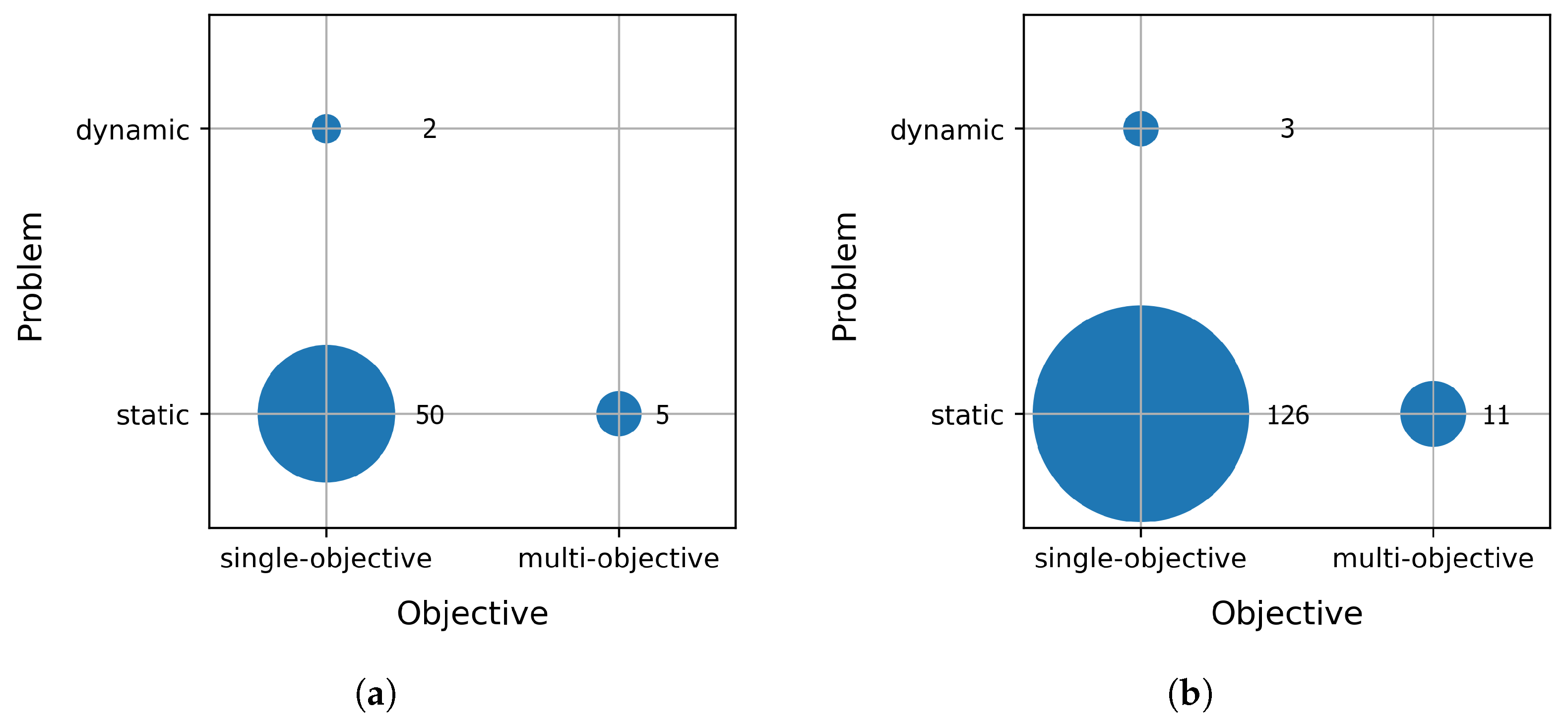
The number of publications per problem type is visualised in Figure 8. Note that the sum of numbers does not necessarily need to be equivalent to the number of included primary studies, as some publications include multiple problem types. This is the case in other bubble charts as well. Single-objective static discrete problems were the most frequent problems in the literature that dealt with attraction basins. Multi-objective problems were less investigated, although continuous domains were slightly better. Research on dynamic problems is almost non-existent. Multi-objective and dynamic problems are more complex, and thus it is understandable that there is a lack of literature on this. We believe that the reason for the lack of literature on multi-objective functions is the not so apparent notion of fitness landscapes. Generally, the fitness landscape is composed of a solution space, an objective space, and the definition of the neighbourhood [24]. In the single-objective functions, the objective space consists of scalars, while in the multi-objective functions, the objective space consists of the vectors of scalars [78]. Therefore, the difficulty in extracting attraction basins in multi-objective functions follows directly from the fact that the attraction basins are derived mainly from fitness landscapes. Interestingly, Figure 8a implies continuous domains are better investigated, but, using the snowballing procedure, this changes. Findings about multi-objective and dynamic problems did not change fundamentally after snowballing.

The numbers of publications regarding the number of objectives and fitness function are presented in Figure 9. Note that we classified the papers which dealt with multi-objectivisation of single-objective problems to both classes (single-objective, and multi-objective). Most of the papers that did not specify the problem type exclusively we classified to single-objective static problems. Such types of problems are easier, and, thus, as Figure 9 suggests, better investigated. Multi-objective dynamic problems were not investigated at all. Including the snowballing procedure or not, this did not have an important impact.

Figure 10 introduces three new classes: An algorithm to compute—meaning the paper provide in some form the algorithm to compute attraction basins; definition—meaning the paper provided a formal definition of attraction basins to some degree; and in-depth—meaning the paper investigated attraction basins more deeply, not just using them. The plot shows the number of publications in relation to the domain of problems (continuous, discrete) and to these new classes. The data show that discrete domains are investigated better. We find this reasonable as it is easier to compute and define attraction basins on discrete problems. Within continuous domains, we rely heavily on discretisation and possibly on a floating-point error. If we choose a better sampling step we risk running out of memory very quickly. Otherwise, it is not easy to obtain sufficient neighbours, while this is quite straightforward within discrete domains. That is, some important neighbours may be missed that lead to another attraction basin. On the other hand, if we decide to sample more neighbours, we risk exceeding the time limit. Nonetheless, attraction basins need to be explored better, especially within continuous domains. As Figure 10 suggests, snowballing only pointed out the differences better.

4.3. RQ3: Definitions Used for Attraction Basins

We found many informal and a few formal definitions of attraction basins that are (dis)similar to various degrees. Here, we list only those that we found fundamentally different from each other (the listing is ordered chronologically):

• Ref. [79]: “A local optimum’s region of attraction is the set of all points in S [search space] which are primarily attracted to it. Regions of attraction may overlap. A local optimum’s strict region of attraction is the set of all points in S which are primarily attracted to it, and are not primarily attracted to any other local optimum. Strict regions of attraction do not overlap.”
• Ref. [80]: “Goldberg (1991) formally defines basins of attraction to a point $x^{*}$ as all points x such that a given hillclimber has a non-zero probability of climbing to within some ε of $x^{*}$ if started within some δ-neigbhorhood of x.”
• Ref. [81]: “A basin of attraction of a vertex $v_n$ is the set of vertices $B_{\varphi }\left(v_n\right)=\{v_0\in V_{\varphi }|\exists$ $v_1,\dots ,v_{n-1}\in V_{\varphi }with{v}_{i+1}\in N_{\varphi }\left(v_i\right)andf\left(v_{i+1}\right)>f\left(v_i\right)(orf\left(v_{i+1}\right)<f\left(v_i\right)ifminimising)foreachi,0\le i<n\}$”, where $V_{\varphi }$ is the set of vertices, $N_{\varphi }$ is the neighbourhood obtained by operator $\varphi$, and $f\left(x\right)$ is the objective function to be optimised.
• Ref. [82]: “The attraction basin of a local optimum $m_j$ is the set of points $\{X_1,\dots ,X_k\}$ of the search space such that a steepest ascent algorithm starting from $X_i(1\le i\le k)$ ends at the local optimum $m_j(\Theta \left(X_i\right)=m_j)$.”
• The previous definition is generalised, i.e., the steepest ascent algorithm is replaced with the so-called pivot rule (any algorithm can be used, including a stochastic one) [83],
• Ref. [84]: “[Attraction basin] … the set of points that can reach the target via neutral or positive mutations.”
• Ref. [85]: “Given a deterministic algorithm A, the basin of attraction $B\left(A\right|s)$ of a point s, is defined as the set of states that, taken as initial states, give origin to trajectories that include point s.”
• Ref. [86]: “The basin of attraction of the local minima are the set of configurations where the cost of flipping a backbone variable is less than the penalty caused by disrupting the associated block cost and cross-linking cost.”
• Ref. [87]: “The basin of attraction of a local minimum is the set of initial conditions which lead, after optimisation, to that minimum.”
• Ref. [88]: “The basin of attraction of a local optimum i is the set $b_i=\{s\in S|LocalSearch\left(s\right)=i\}$.”
• Ref. [32]: “An attraction basin is a region in which there is a single locally optimal point and all other points have their shortest path to reach the locally optimal point.”
• Ref. [89]: “The basin of attraction of the local optimum i is the set $b_i=\{s\in S|p_i\left(s\right)>0\}$.”, where $p_i\left(s\right)$ is the probability that s will end up in i.
• Ref. [29]: “Simply put, they are the areas around the optima that lead directly to the optimum when going downhill (assuming a minimisation problem).”—authors distinguish strong (points that lead exclusively to a single optimum), and weak attraction basins (points that can lead to many optima).
• Ref. [90]: “The attraction basin is defined as the biggest hyper-sphere that contains no valleys around a seed.”
• Ref. [91]: “The basin of attraction of a local optimum is the set of solution candidates from which the focal local optimum can be reached using a number of local search steps (no diversification steps are allowed).”
• Ref. [14]: “An attractor associated with an optimisation algorithm is the ultimate optimal point found by the iterative procedure. When the algorithm converges to an answer, the attractor of the algorithm is a single fixed-point, the simplest type of attractors. Otherwise, it is not a fixed-point attractor. The union of all orbits which converge towards an attractor is called its basin of attraction.”
• Ref. [92]: “Each point in an attraction basin has a monotonic path of increasing (for maxima) or decreasing (for minima) fitness to its local optima.”
• Ref. [15]: “The basin of attraction of the Pareto local solution p, is the set of solutions for which $B\left(p\right)=\{s^{\prime }\in S|p\in maxPLS\left(s^{\prime }\right)\}$”, where maxPLS is the maximal Pareto local search algorithm from [15].

The listed definitions are essentially different from each other because of

• the domain they cover (discrete, real-valued or both),
• the number of objectives in the optimisation problem (single-objective, multi-objective, or both),
• the attraction mechanism they use (steepest ascent, local search, hill-climbing, stochastic algorithm, deterministic algorithm, monotonic increasing/decreasing, any optimisation algorithm, shortest path, etc.),
• the distinguishing between different types of basins (weak or strong, strict or non-strict), or
• the degree of generality.

The main problem with some definitions (e.g., Definitions 3–5, 10, and 17) is that they do not take into account the possibility that the attraction mechanism may reach multiple local optima, e.g., steepest ascent can reach multiple local optima if it finds several neighbours with the same maximum fitness on its way (in this case the algorithm must select a neighbour randomly or in a predetermined order; this, in turn, can lead to different local optima). This problem is solved by introducing two types of attraction basins: strict or non-strict (Definition 1), i.e., weak or strong (Definition 13). Although most of the definitions appear to be general in respect to the type of search space (discrete and real-valued), this is not the case in practice. Definitions do not handle the neighbours and the number of neighbours (sampling) in real-valued domains and the impact this may have on resulting attraction basins. However, this may be regarded as a problem of computation and not a problem of definitions. Definition 2 alleviates this problem by introducing parameters $\epsilon$ and $\delta$. Some definitions handle plateaus (or saddles) differently, e.g., Definition 17 views the plateau as a single point (solution or configuration), and, consequently, escapes each plateau if possible, and therefore sees the plateau as part of an existing attraction basin, that is, each plateau does not define a new attraction basin. This is not the case with, e.g., Definition 10, where plateaus are not escaped, and the algorithm (local search) stops at the plateau (local optimum), which means a new attraction basin must be defined. We identify the lack of a general theoretical framework of attraction basins that will unite different views/definitions in a meaningful way, and investigate all domains and problem types better. Only then, can the concept be exploited fully. We found that, without snowballing, many important definitions of attraction basins would be missed (Definitions 1, 2, 13, and 14).

4.4. RQ4: Algorithms Used for Attraction Basins

Considering that relatively many definitions have been used so far, we would expect to find efficient algorithms to compute attraction basins, but this is not the case. Only a few algorithms have been developed and are often described poorly. The simplest and most popular algorithm is based on exhaustive enumeration of a search space, where a local search procedure is run for each candidate solution. The most used local search procedures are Best Improvement, and First Improvement (see Algorithm A1 in Appendix A), e.g., in [89]. The only difference is that Best Improvement selects the best neighbour, while First Improvement selects the first neighbour better than the current solution, encountered on its way to the optimum. Once all local searches reach their optima, it is easy to determine attraction basins, for example, each candidate solution could be labelled by its optimum. However, this algorithm, without additional sophistication, handles plateaus poorly. Once it reaches a single point from the plateau it will stop and create a new basin if this point is not reached by other runs. This means multiple points on the same plateau may create multiple basins. If we are within the real-valued domains, the number of basins may increase due to the thinner sampling step. Even if we solve this problem, for each plateau we will have one basin, as the algorithm cannot escape the plateau. This may be correct behaviour for some definitions of attraction basins (e.g., Definition 10), but not for others (e.g., Definition 17). In terms of the time complexity, the efficient technique to compute attraction basins comes from T. Jones and G. Rawlins [93] in 1993 (see Algorithm A2 in Appendix A). The idea is based on depth-first search and so-called reverse hill climbing, where, starting from the optima, the algorithm builds its attraction basins recursively using the lookup table. This algorithm must be run for each optimum. This is a drawback for problems where it is impossible to know all the optima in advance (real-valued domains). S.W. Mahfoud [79], in the same year, published the algorithm which returns the set of local optima to which a point is closest, even in the case of large plateaus (see Algorithm A3 in Appendix A). Once the algorithm finds one or more optima, the result could be used in a similar manner as before, that is, each candidate solution could be labelled by its local optima (notice the plural). M. Van Turnhout and F. Bociort, in their optical system optimisation [87], report on the use of an algorithm that starts with following the gradient downwards by solving Equation (3), where the vector x is a point in the two-dimensional solution space, and $\mathrm{d}s$ is the arc length along the curved continuous path.

$$\frac{\mathrm{d}x}{\mathrm{d}s}=-\frac{▿MF}{\parallel ▿MF\parallel },x=(c_2,c_3),\mathrm{d}s=\sqrt{{\parallel \mathrm{d}x\parallel }^2}$$

(3)

The input to the algorithm is the grid of equally spaced starting points in the plane $(c_2,c_3)$. Depending on which local minimum the algorithm obtains, the starting point is coloured with the corresponding colour for that minimum. Using the same input, the authors of [22] computed attraction basins for real-valued domains in three steps (see Algorithm A4 in Appendix A). First, the potential borders of the attraction basins are obtained (lines 2–7), followed by a boundary fill step (lines 8–11), and, last, removal of the false borders (lines 12–18). We found that, without snowballing, two algorithms would be missed: Algorithms A2 and A3 from Appendix A.

Estimation/approximation algorithms have also been used to compute attraction basins. They are based on clustering [94,95], the detect-multimodal method followed by hyper-spheres [90], sampling and area division [96], tabu zones of different forms and sizes, and with different locations in relation to the corresponding optima [97], and based on sampling along each dimensional axis until finding a slump in fitness and then creating a hyper-rectangle [98]. Most of these algorithms assume real-valued domain problems, but, still, there is a lack of exact and efficient algorithms to evaluate them. Therefore, we did not examine them more closely in this work.

4.5. RQ5: Most Popular Topics for Attraction Basins

Table 2. Contexts and purposes for which attraction basins were used.

Fitness landscape analysis, problem difficulty	e.g., [28,32,105]
Clustering, niching associated with attraction basins	e.g., [94,99,100]
Exploration, exploitation, diversification, intensification	e.g., [22,76,77]
Problem generation	[106]
Problem visualisation	e.g., [78,107,108]
Comparison, performance, analysis of metaheuristics	e.g., [31,79,109]
Basins within the metaheuristic to enhance the search	e.g., [96,97,110]
Local Optima Networks	e.g., [88,111,112]
Automated Algorithm Selection	[35]

lists the contexts/purposes where attraction basins were investigated. They are used mostly for Fitness Landscape Analysis (i.e., Exploratory Landscape Analysis, search space analysis). Note that attraction basins within the continuous domain were often used for clustering and niching. Different clusters and niches were often considered as approximated attraction basins [99,100]; however, this is in contrast with the usual definition. Therefore, we found the “usual” attraction basins to be less investigated within the continuous domain. Recently, attraction basins have received attention for analysis of exploration and exploitation. Moving between different attraction basins was perceived as exploration, and moving within the same attraction basin as exploitation [22,76,101]. Some works altered the inner workings of metaheuristics to control moving between attraction basins, such as the detect multimodal and radius-based methods [90,102]. A lot of works used attraction basins to measure problem difficulty, e.g., the number and distribution of attraction basins sizes, ratios between global optima attraction basins sizes, and local optima attraction basins sizes [30,75,94,103,104]. We recognised the lack of a general framework that would organise all such approaches within the field in a systematic manner. The only topic found after performing the snowballing was automatic algorithm selection, however, with only one publication. Automatic algorithm selection means, instead of analysis and experimentation with optimisation algorithms, we let software select the best algorithm for concrete problems by learning (e.g., using Machine Learning), based on the features such as number of attraction basins, distribution of their sizes, etc. [35]. Although, as this SMS reveals, the attraction basins were used for many important topics and purposes in the field of metaheuristics, we found no study that investigates the influence of different definitions and algorithms on the attraction basins and their usability on the topic. The authors of [87,89] investigate only the influence of local search algorithms on the resulting attraction basins in certain domains. However, their impact on the purpose for which attraction basins are used is never discussed. This work emphasises the importance of this investigation by highlighting the different definitions and algorithms to compute attraction basins, and the different contexts where attraction basins have been used.

4.6. RQ6: Demographic Data of SMS

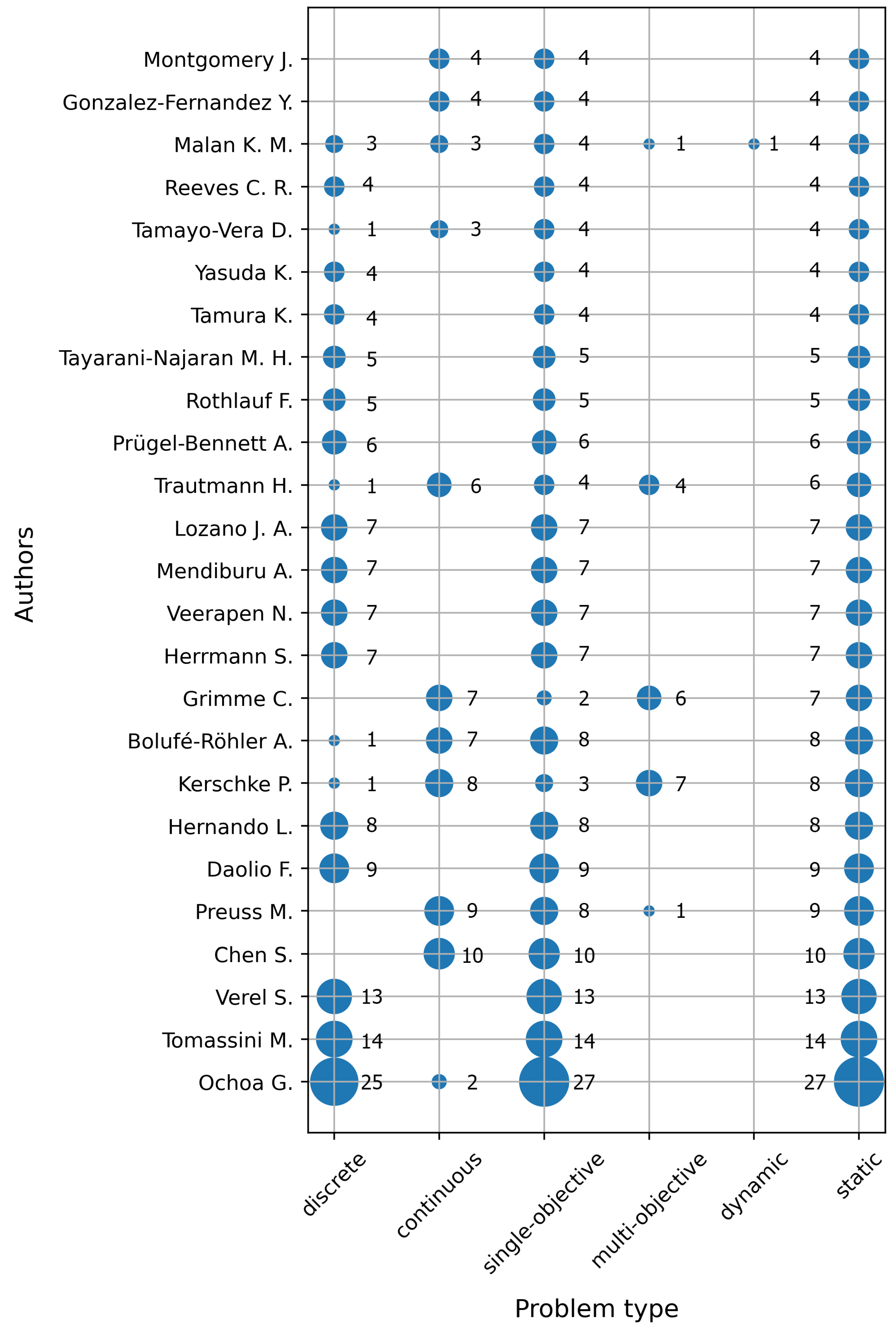
The most prolific authors are Ochoa G., Tomassini M., Verel S., and Chen S. as Figure 11 suggests. Ochoa G., Tomassini M., and Verel S., usually in a group, published the most papers on Local Optima Networks [113], while Chen S. on threshold convergence and exploration [25,114]. It seems that Local Optima Networks have received a lot of attention in the research community. A local optima network is a graph where each node represents a local optimum, and each edge between two nodes represents the probability to pass from one attraction basin to another [115].

Next, we show the most popular venues that publish articles relevant to our topic. Figure 12 shows the publication count per journal. We merged journals that published less than two studies to the category “other” due to space limitations. The Evolutionary Computation journal published the most papers (13), followed immediately by IEEE Transactions on Evolutionary Computation (8).

The Genetic and Evolutionary Computation Conference (GECCO)—19, and the IEEE Congress on Evolutionary Computation (CEC)—18, published the most conference papers on the topic of attraction basins (see Figure 13). Conferences publish more papers on the topic than journals, as Figure 13 suggests. In the Figure 13, we merged conferences that published less than two studies to the category “other”.

Publication count by year is shown in Figure 14. Note, only papers accepted before July 2021 were considered. The usage of attraction basins increased in the last decade. One of the reasons behind this is the exploitation of high computing capabilities, as the search spaces are too enormous to compute attraction basins exactly.

4.7. Necessity of Snowballing

As indicated earlier in this section, we investigated what happens to the results after the inclusion of new synonyms in the search string, together with iterative forward and backward snowballing. As expected, the number of papers increased enormously, from 201 to 1574 in Scopus, and from 105 to 966 in the Web of Science database. However, only 38 articles remained after screening. This is due to the imprecise term basin, which is responsible, e.g., for including the papers that deal with rivers and lakes (e.g., geology). Strangely, refinement/filtering did not exclude these papers during the database search. Demographic data followed almost the same distribution as before including the new synonyms. Only one new journal with more than two articles was identified (Journal of Global Optimization). This journal mainly published papers on the important topic of the filled functions. Filled functions are the auxiliary functions that help algorithms to escape local minima by optimising these new functions. This important topic would not be identified without changing the search string. Interestingly, using the snowballing on the article that deals with filled functions, we followed the track back to 1987, where attraction basins were mentioned. Again, the topic was filled functions, which may imply that this is the first context where attraction basins were used. During the full-text read we found that in the paper [116], the authors wrote: “The idea about the basin appeared in the 1970s (Dixon et al., 1976)”; however, we did not find this manuscript available in the full-text. Conclusions about problem types stays the same, although the numbers went slightly higher for continuous domains. Almost all these new papers that dealt with continuous domains had filled functions as their topic. For some reason, the frequency of papers that deal with this newly identified topic dropped in last decade. During the extraction of data, surprisingly, we found the new synonyms as well, although not so often used, “attraction area”, “attraction region”, “basin of convergence”, “region of convergence”, and “catchment basin”. The frequency of the term “basin” increased again, because of the topic of filled functions. After adding the latest new synonyms to our search string, we did not find any new relevant articles (all of them were from other fields). Overall, we estimate that, in this work, snowballing was important and necessary. Otherwise, some important definitions and algorithms would have been missed. Terms other than “basin of attraction” and “attraction basin” would not be found. The important topic of filled functions wouldn’t be identified at all. We found it only after including the new synonyms (first time) and performing snowballing. We would not have found that the idea of attraction basins traces its roots back to the 1970s according to the work in [116].

5. Conclusions

In this study, we were limited to Computer Science, although the study is useful to other areas as well, such as physics and mathematics, where the attraction basins are examined in the context of dynamical systems. Only two databases—Scopus and ISI Web of Science—were used to construct the seed set. We omitted the papers published in workshops, dissertations, and the rest of the grey literature. Our SMS included categories that are of a similar level of granularity. Specific categories, such as dimensionality of the problem or specific types of discrete spaces (combinatorial, permutation, binary), are not considered in this SMS.

In this paper, we presented the first SMS on attraction basins in the field of metaheuristics. We believe this study will help newcomers, as well as those who are experienced, to dive into the topic more quickly, and therefore enhance the improvement in the field. The main findings on the topic are as follows:

• Discrete domains were investigated far better than continuous.
• Single-objective static problems dominated. Multi-objective problems were investigated better within the continuous domain, although still very weakly.
• Different definitions of attraction basins were used, while the most frequent one was based on a local search. Within the continuous domain researchers often use clusters or niches as approximated attraction basins. There is a lack of a general framework of attraction basins in the field of metaheuristics.
• Only a few “exact” algorithms were found, exhaustive enumeration with local search, reverse hillclimbing, and the primary attraction algorithm. No parallel and scalable algorithm was found to compute attraction basins.
• Attraction basins were used for many purposes, such as fitness landscape analysis, clustering and niching, comparison of metaheuristics, exploration and exploitation, and analysis of metaheuristics, to enhance the search, problem generation, filled functions, etc. Local Optima Network is the topic that received the most attention in the area regarding the attraction basins.
• The notion of attraction basins first appeared in the 1970s.

Regarding the question of whether is it necessary to perform snowballing, we answer ’yes’ for some works (it holds for this work).

We encourage researchers to develop efficient, parallel, and scalable algorithms to compute attraction basins that can run on a cluster [117,118,119,120,121]. However, an unambiguous definition of attraction basins is needed to design an algorithm. Unfortunately, often weak definitions are provided that do not take into account all specificities. This is especially a problem within the continuous domain. Attraction basins on the continuous domain are understood poorly. These specificities include the settings, such as the neighbourhood definition, order of neighbours, specific local search variant, and sampling. The bigger impact of these settings on the resulting attraction basins could have huge repercussions on the attraction basin’s applications. Therefore, as our future work, we will investigate the impact of these different settings on the resulting attraction basins. We will investigate the impact of shifting, rotating, and adding more dimensions to problems on attraction basins. Further, we will analyse the influence of different settings on the exploration and exploitation metric proposed in [22]. If we find out a significant influence, the metric will be revised in one of our future works. Therefore, we encourage researchers to experiment with different definitions/algorithms, and provide a general framework that is independent of an attraction mechanism, attractor, and initial configurations. In this way, the power of the concept may be exploited better.

References

1. Ellison, G. Basins of Attraction, Long-Run Stochastic Stability, and the Speed of Step- by-Step Evolution. Rev. Econ. Stud. 2000, 67, 17–45. [Google Scholar] [CrossRef] [Green Version]
2. Page, F.H.; Wooders, M.H. Strategic Basins of Attraction, the Farsighted Core, and Network Formation Games; Technical Report; University of Warwick—Department of Economics: Coventry, UK, 2005. [Google Scholar]
3. Vicario, E. Imitation and Local Interactions: Long Run Equilibrium Selection. Games 2021, 12, 30. [Google Scholar] [CrossRef]
4. Scott, M.; Neta, B.; Chun, C. Basin attractors for various methods. Appl. Math. Comput. 2011, 218, 2584–2599. [Google Scholar] [CrossRef]
5. Cordero, A.; Soleymani, F.; Torregrosa, J.; Shateyi, S. Basins of Attraction for Various Steffensen-Type Methods. J. Appl. Math. 2014, 2014, 539707. [Google Scholar] [CrossRef]
6. Zotos, E.; Sanam Suraj, M.; Mittal, A.; Aggarwal, R. Comparing the Geometry of the Basins of Attraction, the Speed and the Efficiency of Several Numerical Methods. Int. J. Appl. Comput. Math. 2018, 4, 105. [Google Scholar] [CrossRef] [Green Version]
7. Demongeot, J.; Goles, E.; Morvan, M.; Noual, M.; Sené, S. Attraction Basins as Gauges of Robustness against Boundary Conditions in Biological Complex Systems. PLoS ONE 2010, 5, e0011793. [Google Scholar] [CrossRef] [PubMed]
8. Gardiner, J. Evolutionary basins of attraction and convergence in plants and animals. Commun. Integr. Biol. 2013, 6, e26760. [Google Scholar] [CrossRef]
9. Conforte, A.J.; Alves, L.; Coelho, F.C.; Carels, N.; Da Silva, F.A.B. Modeling Basins of Attraction for Breast Cancer Using Hopfield Networks. Front. Genet. 2020, 11, 314. [Google Scholar] [CrossRef] [PubMed] [Green Version]
10. Isomäki, H.M.; Von Boehm, J.; Räty, R. Fractal basin boundaries of an impacting particle. Phys. Lett. A 1988, 126, 484–490. [Google Scholar] [CrossRef]
11. Xu, N.; Frenkel, D.; Liu, A.J. Direct Determination of the Size of Basins of Attraction of Jammed Solids. Phys. Rev. Lett. 2011, 106, 245502. [Google Scholar] [CrossRef] [Green Version]
12. Guseva, K.; Feudel, U.; Tél, T. Influence of the history force on inertial particle advection: Gravitational effects and horizontal diffusion. Phys. Rev. E 2013, 88, 042909. [Google Scholar] [CrossRef] [Green Version]
13. Pitzer, E.; Affenzeller, M.; Beham, A. A closer look down the basins of attraction. In Proceedings of the 2010 UK Workshop on Computational Intelligence, Colchester, UK, 8–10 September 2010; pp. 1–6. [Google Scholar]
14. Tsang, K.K. Basin of Attraction as a measure of robustness of an optimization algorithm. In Proceedings of the 2018 14th International Conference on Natural Computation, Fuzzy Systems and Knowledge Discovery, Huangshan, China, 28–30 July 2018; pp. 133–137. [Google Scholar]
15. Drugan, M.M. Estimating the number of basins of attraction of multi-objective combinatorial problems. J. Comb. Optim. 2019, 37, 1367–1407. [Google Scholar] [CrossRef]
16. Gogna, A.; Tayal, A. Metaheuristics: Review and application. J. Exp. Theor. Artif. Intell. 2013, 25, 503–526. [Google Scholar] [CrossRef]
17. Back, T.; Fogel, D.B.; Michalewicz, Z. Handbook of Evolutionary Computation, 1st ed.; Institute of Physics Publishing: Bristol, UK, 1997. [Google Scholar]
18. Eiben, A.E.; Smith, J.E. Introduction to Evolutionary Computing, 2nd ed.; Springer: Berlin/Heidelberg, Germany, 2015. [Google Scholar]
19. Cai, X.; Hu, Z.; Zhao, P.; Zhang, W.; Chen, J. A hybrid recommendation system with many-objective evolutionary algorithm. Expert Syst. Appl. 2020, 159, 113648. [Google Scholar] [CrossRef]
20. Li, J.Y.; Zhan, Z.H.; Wang, C.; Jin, H.; Zhang, J. Boosting Data-Driven Evolutionary Algorithm with Localized Data Generation. IEEE Trans. Evol. Comput. 2020, 24, 923–937. [Google Scholar] [CrossRef]
21. Einakian, S.; Newman, T.S. An examination of color theories in map-based information visualization. J. Comput. Lang. 2019, 51, 143–153. [Google Scholar] [CrossRef]
22. Jerebic, J.; Mernik, M.; Liu, S.H.; Ravber, M.; Baketarić, M.; Mernik, L.; Črepinšek, M. A novel direct measure of exploration and exploitation based on attraction basins. Expert Syst. Appl. 2021, 167, 114353. [Google Scholar] [CrossRef]
23. Caamaño, P.; Prieto, A.; Becerra, J.A.; Bellas, F.; Duro, R.J. Real-Valued Multimodal Fitness Landscape Characterization for Evolution. In Neural Information Processing. Theory and Algorithms; Wong, K.W., Mendis, B.S.U., Bouzerdoum, A., Eds.; Springer: Berlin/Heidelberg, Germany, 2010; pp. 567–574. [Google Scholar]
24. Malan, K.M.; Engelbrecht, A.P. A Survey of Techniques for Characterising Fitness Landscapes and Some Possible Ways Forward. Inf. Sci. 2013, 241, 148–163. [Google Scholar] [CrossRef] [Green Version]
25. Chen, S.; Bolufé-Röhler, A.; Montgomery, J.; Hendtlass, T. An Analysis on the Effect of Selection on Exploration in Particle Swarm Optimization and Differential Evolution. In Proceedings of the 2019 IEEE Congress on Evolutionary Computation, Wellington, New Zealand, 10–13 June 2019; pp. 3037–3044. [Google Scholar]
26. Wright, S. The Roles of Mutation Inbreeding, Crossbreeding and Selection in Evolution. In Proceedings of the Sixth International Congress on Genetics, Ithaca, NY, USA, 24–31 August 1932; Brooklyn Botanic Garden: New York, NY, USA, 1932; Volume 1. [Google Scholar]
27. Mersmann, O.; Preuss, M.; Trautmann, H. Benchmarking Evolutionary Algorithms: Towards Exploratory Landscape Analysis. In Parallel Problem Solving from Nature, PPSN XI; Schaefer, R., Cotta, C., Kołodziej, J., Rudolph, G., Eds.; Springer: Berlin/Heidelberg, Germany, 2010; pp. 73–82. [Google Scholar]
28. Muñoz, M.A.; Kirley, M.; Halgamuge, S.K. Landscape characterization of numerical optimization problems using biased scattered data. In Proceedings of the 2012 IEEE Congress on Evolutionary Computation, Brisbane, Australia, 10–15 June 2012; pp. 1–8. [Google Scholar]
29. Pitzer, E.; Affenzeller, M. A Comprehensive Survey on Fitness Landscape Analysis. In Recent Advances in Intelligent Engineering Systems; Springer: Berlin/Heidelberg, Germany, 2012; pp. 161–191. [Google Scholar]
30. Tayarani-N, M.H.; Prügel-Bennett, A. An Analysis of the Fitness Landscape of Travelling Salesman Problem. Evol. Comput. 2016, 24, 347–384. [Google Scholar] [CrossRef] [PubMed] [Green Version]
31. Merz, P. Advanced Fitness Landscape Analysis and the Performance of Memetic Algorithms. Evol. Comput. 2004, 12, 303–325. [Google Scholar] [CrossRef] [PubMed]
32. Xin, B.; Chen, J.; Pan, F. Problem Difficulty Analysis for Particle Swarm Optimization: Deception and Modality. In Proceedings of the First ACM/SIGEVO Summit on Genetic and Evolutionary Computation, Shanghai, China, 12–14 June 2009; Association for Computing Machinery: New York, NY, USA, 2009; pp. 623–630. [Google Scholar]
33. Mersmann, O.; Bischl, B.; Trautmann, H.; Preuss, M.; Weihs, C.; Rudolph, G. Exploratory Landscape Analysis. In Proceedings of the 13th Annual Conference on Genetic and Evolutionary Computation, Dublin, Ireland, 12–16 July 2011; Association for Computing Machinery: New York, NY, USA, 2011; pp. 829–836. [Google Scholar]
34. Rodriguez-Maya, N.E.; Graff, M.; Flores, J.J. Performance Classification of Genetic Algorithms on Continuous Optimization Problems. In Nature-Inspired Computation and Machine Learning; Gelbukh, A., Espinoza, F.C., Galicia-Haro, S.N., Eds.; Springer International Publishing: Cham, Switzerland, 2014; pp. 1–12. [Google Scholar]
35. Kerschke, P.; Hoos, H.H.; Neumann, F.; Trautmann, H. Automated Algorithm Selection: Survey and Perspectives. Evol. Comput. 2019, 27, 3–45. [Google Scholar] [CrossRef] [PubMed]
36. Liefooghe, A.; Verel, S.; Lacroix, B.; Zăvoianu, A.C.; McCall, J. Landscape Features and Automated Algorithm Selection for Multi-Objective Interpolated Continuous Optimisation Problems. In Proceedings of the Genetic and Evolutionary Computation Conference, Lille, France, 10–14 July 2021; Association for Computing Machinery: New York, NY, USA, 2021; pp. 421–429. [Google Scholar]
37. Eiben, A.E.; Schippers, C.A. On Evolutionary Exploration and Exploitation. Fundam. Inform. 1998, 35, 35–50. [Google Scholar] [CrossRef]
38. Ollion, C.; Doncieux, S. Why and How to Measure Exploration in Behavioral Space. In Proceedings of the 13th Annual Conference on Genetic and Evolutionary Computation, Dublin, Ireland, 12–16 July 2011; Association for Computing Machinery: New York, NY, USA, 2011; pp. 267–274. [Google Scholar]
39. Črepinšek, M.; Liu, S.H.; Mernik, M. Exploration and Exploitation in Evolutionary Algorithms: A Survey. ACM Comput. Surv. 2013, 45, 1–33. [Google Scholar] [CrossRef]
40. Xu, J.; Zhang, J. Exploration-exploitation tradeoffs in metaheuristics: Survey and analysis. In Proceedings of the 33rd Chinese Control Conference, Nanjing, China, 28–30 July 2014; pp. 8633–8638. [Google Scholar]
41. Squillero, G.; Tonda, A. Divergence of character and premature convergence: A survey of methodologies for promoting diversity in evolutionary optimization. Inf. Sci. 2016, 329, 782–799. [Google Scholar] [CrossRef] [Green Version]
42. Kitchenham, B.; Pretorius, R.; Budgen, D.; Pearl Brereton, O.; Turner, M.; Niazi, M.; Linkman, S. Systematic literature reviews in software engineering—A tertiary study. Inf. Softw. Technol. 2010, 52, 792–805. [Google Scholar] [CrossRef]
43. Petersen, K.; Vakkalanka, S.; Kuzniarz, L. Guidelines for conducting systematic mapping studies in software engineering: An update. Inf. Softw. Technol. 2015, 64, 1–18. [Google Scholar] [CrossRef]
44. Kosar, T.; Bohra, S.; Mernik, M. Domain-Specific Languages: A Systematic Mapping Study. Inf. Softw. Technol. 2016, 71, 77–91. [Google Scholar] [CrossRef]
45. Kitchenham, B.A.; Dyba, T.; Jorgensen, M. Evidence-Based Software Engineering. In Proceedings of the 26th International Conference on Software Engineering, Edinburgh, UK, 28–28 May 2004; IEEE Computer Society: Washington, DC, USA, 2004; pp. 273–281. [Google Scholar]
46. Dyba, T.; Kitchenham, B.; Jorgensen, M. Evidence-based software engineering for practitioners. IEEE Softw. 2005, 22, 58–65. [Google Scholar] [CrossRef] [Green Version]
47. Jorgensen, M.; Dyba, T.; Kitchenham, B. Teaching evidence-based software engineering to university students. In Proceedings of the 11th IEEE International Software Metrics Symposium, Washington, DC, USA, 19–22 September 2005; Volume 2005, p. 24. [Google Scholar]
48. Choraś, M.; Demestichas, K.; Giełczyk, A.; Herrero, A.; Ksieniewicz, P.; Remoundou, K.; Urda, D.; Woźniak, M. Advanced Machine Learning techniques for fake news (online disinformation) detection: A systematic mapping study. Appl. Soft Comput. 2021, 101, 107050. [Google Scholar] [CrossRef]
49. Houssein, E.H.; Gad, A.G.; Wazery, Y.M.; Suganthan, P.N. Task Scheduling in Cloud Computing based on Meta-heuristics: Review, Taxonomy, Open Challenges, and Future Trends. Swarm Evol. Comput. 2021, 62, 100841. [Google Scholar] [CrossRef]
50. Ferranti, N.; Rosário Furtado Soares, S.S.; De Souza, J.F. Metaheuristics-based ontology meta-matching approaches. Expert Syst. Appl. 2021, 173, 114578. [Google Scholar] [CrossRef]
51. Dragoi, E.N.; Dafinescu, V. Review of Metaheuristics Inspired from the Animal Kingdom. Mathematics 2021, 9, 2335. [Google Scholar] [CrossRef]
52. Kitchenham, B.; Brereton, P.; Budgen, D. The Educational Value of Mapping Studies of Software Engineering Literature. In Proceedings of the 32nd ACM/IEEE International Conference on Software Engineering, Cape Town, South Africa, 1–8 May 2010; Association for Computing Machinery: New York, NY, USA, 2010; pp. 589–598. [Google Scholar]
53. Felizardo, K.R.; De Souza, E.F.; Napoleão, B.M.; Vijaykumar, N.L.; Baldassarre, M.T. Secondary studies in the academic context: A systematic mapping and survey. J. Syst. Softw. 2020, 170, 110734. [Google Scholar] [CrossRef]
54. Kitchenham, B.A.; Budgen, D.; Brereton, O.P. The Value of Mapping Studies: A Participant observer Case Study. In Proceedings of the 14th International Conference on Evaluation and Assessment in Software Engineering, London, UK, 13–14 May 2014; BCS Learning & Development Ltd.: Swindon, UK, 2010; pp. 25–33. [Google Scholar]
55. Wohlin, C.; Runeson, P.; Da Mota Silveira Neto, P.A.; Engström, E.; Do Carmo Machado, I.; De Almeida, E.S. On the reliability of mapping studies in software engineering. J. Syst. Softw. 2013, 86, 2594–2610. [Google Scholar] [CrossRef] [Green Version]
56. Kosar, T.; Bohra, S.; Mernik, M. A Systematic Mapping Study driven by the margin of error. J. Syst. Softw. 2018, 144, 439–449. [Google Scholar] [CrossRef]
57. Wohlin, C. Guidelines for Snowballing in Systematic Literature Studies and a Replication in Software Engineering. In Proceedings of the 18th International Conference on Evaluation and Assessment in Software Engineering, London, UK, 13–14 May 2014; Association for Computing Machinery: New York, NY, USA, 2014; pp. 1–10. [Google Scholar]
58. Mourão, E.; Pimentel, J.F.; Murta, L.; Kalinowski, M.; Mendes, E.; Wohlin, C. On the performance of hybrid search strategies for systematic literature reviews in software engineering. Inf. Softw. Technol. 2020, 123, 106294. [Google Scholar] [CrossRef]
59. Dieste, O.; Padua, A.G. Developing Search Strategies for Detecting Relevant Experiments for Systematic Reviews. In Proceedings of the First International Symposium on Empirical Software Engineering and Measurement, Madrid, Spain, 20–21 September 2007; pp. 215–224. [Google Scholar]
60. Kitchenham, B.; Charters, S. Guidelines for Performing Systematic Literature Reviews in Software Engineering; Technical Report, Keele University and Durham University Joint Report; EBSE: Goyang, Korea, 2007. [Google Scholar]
61. Petersen, K.; Feldt, R.; Mujtaba, S.; Mattsson, M. Systematic Mapping Studies in Software Engineering. In Proceedings of the 12th International Conference on Evaluation and Assessment in Software Engineering, Bari, Italy, 26–27 June 2008; BCS Learning & Development Ltd.: Swindon, UK, 2008; pp. 68–77. [Google Scholar]
62. Rožanc, I.; Mernik, M. The screening phase in systematic reviews: Can we speed up the process? In Advances in Computers; Hurson, A.R., Ed.; Elsevier: Amsterdam, The Netherlands, 2021; Volume 123, pp. 115–191. [Google Scholar] [CrossRef]
63. Garousi, V.; Felderer, M.; Mäntylä, M.V. Guidelines for including grey literature and conducting multivocal literature reviews in software engineering. Inf. Softw. Technol. 2019, 106, 101–121. [Google Scholar] [CrossRef] [Green Version]
64. Kamei, F.; Wiese, I.; Lima, C.; Polato, I.; Nepomuceno, V.; Ferreira, W.; Ribeiro, M.; Pena, C.; Cartaxo, B.; Pinto, G.; et al. Grey Literature in Software Engineering: A critical review. Inf. Softw. Technol. 2021, 138. [Google Scholar] [CrossRef]
65. Nepomuceno, V.; Soares, S. On the need to update systematic literature reviews. Inf. Softw. Technol. 2019, 109, 40–42. [Google Scholar] [CrossRef]
66. Osman, I.H.; Kelly, J.P. Meta-Heuristics: An Overview. In Meta-Heuristics: Theory and Applications; Springer US: Boston, MA, USA, 1996; pp. 1–21. [Google Scholar]
67. Črepinšek, M.; Mernik, M.; Javed, F.; Bryant, B.R.; Sprague, A. Extracting Grammar from Programs: Evolutionary Approach. ACM SIGPLAN Not. 2005, 40, 39–46. [Google Scholar] [CrossRef]
68. Kovačević, Ž.; Mernik, M.; Ravber, M.; Črepinšek, M. From Grammar Inference to Semantic Inference—An Evolutionary Approach. Mathematics 2020, 8, 816. [Google Scholar] [CrossRef]
69. Dorigo, M.; Maniezzo, V.; Colorni, A. Ant system: Optimization by a colony of cooperating agents. IEEE Trans. Syst. Man Cybern. Part B 1996, 26, 29–41. [Google Scholar] [CrossRef] [Green Version]
70. Dorigo, M.; Birattari, M.; Stützle, T. Ant Colony Optimization: Artificial Ants as a Computational Intelligence Technique. IEEE Comput. Intell. Mag. 2006, 1, 28–39. [Google Scholar] [CrossRef]
71. Dasgupta, D.; Michalewicz, Z. Evolutionary Algorithms—An Overview. In Evolutionary Algorithms in Engineering Applications; Dasgupta, D., Michalewicz, Z., Eds.; Springer: Berlin/Heidelberg, Germany, 1997; pp. 3–28. [Google Scholar]
72. Wolpert, D.; Macready, W. No free lunch theorems for optimization. IEEE Trans. Evol. Comput. 1997, 1, 67–82. [Google Scholar] [CrossRef] [Green Version]
73. Tangherloni, A.; Spolaor, S.; Cazzaniga, P.; Besozzi, D.; Rundo, L.; Mauri, G.; Nobile, M. Biochemical parameter estimation vs. benchmark functions: A comparative study of optimization performance and representation design. Appl. Soft Comput. J. 2019, 81, 105494. [Google Scholar] [CrossRef]
74. Malan, K.M. A Survey of Advances in Landscape Analysis for Optimisation. Algorithms 2021, 14, 40. [Google Scholar] [CrossRef]
75. Hernando, L.; Mendiburu, A.; Lozano, J.A. Anatomy of the Attraction Basins: Breaking with the Intuition. Evol. Comput. 2019, 27, 435–466. [Google Scholar] [CrossRef] [Green Version]
76. Bolufé-Röhler, A.; Tamayo-Vera, D.; Chen, S. An LaF-CMAES hybrid for optimization in multi-modal search spaces. In Proceedings of the 2017 IEEE Congress on Evolutionary Computation, San Sebastian, Spain, 5–8 June 2017; pp. 757–764. [Google Scholar]
77. Gonzalez-Fernandez, Y.; Chen, S. Identifying and Exploiting the Scale of a Search Space in Particle Swarm Optimization. In Proceedings of the 2014 Annual Conference on Genetic and Evolutionary Computation, Vancouver, BC, Canada, 12–16 July 2014; Association for Computing Machinery: New York, NY, USA, 2014; pp. 17–24. [Google Scholar]
78. Kerschke, P.; Grimme, C. An Expedition to Multimodal Multi-objective Optimization Landscapes. In Evolutionary Multi-Criterion Optimization; Trautmann, H., Rudolph, G., Klamroth, K., Schütze, O., Wiecek, M., Jin, Y., Grimme, C., Eds.; Springer International Publishing: Cham, Switzerland, 2017; pp. 329–343. [Google Scholar]
79. Mahfoud, S.W. Simple Analytical Models of Genetic Algorithms for Multimodal Function Optimization. In Proceedings of the 5th International Conference on Genetic Algorithms, Urbana, IL, USA, 17–21 July 1993; Morgan Kaufmann Publishers Inc.: San Francisco, CA, USA, 1993; p. 643. [Google Scholar]
80. Horn, J.; Goldberg, D.E. Genetic Algorithm Difficulty and the Modality of Fitness Landscapes. In Foundations of Genetic Algorithms; Whitley, L.D., Vose, M.D., Eds.; Elsevier: Amsterdam, The Netherlands, 1995; Volume 3, pp. 243–269. [Google Scholar]
81. Vassilev, V.K.; Fogarty, T.C.; Miller, J.F. Information Characteristics and the Structure of Landscapes. Evol. Comput. 2000, 8, 31–60. [Google Scholar] [CrossRef] [PubMed]
82. Garnier, J.; Kallel, L. How to Detect all Maxima of a Function. In Theoretical Aspects of Evolutionary Computing; Springer: Berlin/Heidelberg, Germany, 2001; pp. 343–370. [Google Scholar]
83. Anderson, E.J. Markov chain modelling of the solution surface in local search. J. Oper. Res. Soc. 2002, 53, 630–636. [Google Scholar] [CrossRef]
84. Wiles, J.; Tonkes, B. Mapping the Royal Road and Other Hierarchical Functions. Evol. Comput. 2003, 11, 129–149. [Google Scholar] [CrossRef]
85. Prestwich, S.; Roli, A. Symmetry Breaking and Local Search Spaces. In Proceedings of the Second International Conference on Integration of AI and OR Techniques in Constraint Programming for Combinatorial Optimization Problems, Prague, Czech Republic, 31 May–1 June 2005; Springer: Berlin/Heidelberg, Germany, 2005; pp. 273–287. [Google Scholar]
86. Prügel-Bennett, A. Finding Critical Backbone Structures with Genetic Algorithms. In Proceedings of the 9th Annual Conference on Genetic and Evolutionary Computation, London, UK, 7–11 July 2007; Association for Computing Machinery: New York, NY, USA, 2007; pp. 1343–1348. [Google Scholar]
87. Van Turnhout, M.; Bociort, F. Predictability and unpredictability in optical system optimization. In Current Developments in Lens Design and Optical Engineering VIII; Mouroulis, P.Z., Smith, W.J., Johnson, R.B., Eds.; SPIE: Bellingham, WA, USA, 2007; Volume 6667, pp. 63–70. [Google Scholar]
88. Ochoa, G.; Tomassini, M.; Vérel, S.; Darabos, C. A Study of NK Landscapes’ Basins and Local Optima Networks. In Proceedings of the 10th Annual Conference on Genetic and Evolutionary Computation, Atlanta, GA, USA, 12–16 July 2008; Association for Computing Machinery: New York, NY, USA, 2008; pp. 555–562. [Google Scholar]
89. Ochoa, G.; Verel, S.; Tomassini, M. First-Improvement vs. Best-Improvement Local Optima Networks of NK Landscapes. In Parallel Problem Solving from Nature; Schaefer, R., Cotta, C., Kołodziej, J., Rudolph, G., Eds.; Springer: Berlin/Heidelberg, Germany, 2010; pp. 104–113. [Google Scholar]
90. Xu, Z.; Polojärvi, M.; Yamamoto, M.; Furukawa, M. Attraction basin estimating GA: An adaptive and efficient technique for multimodal optimization. In Proceedings of the 2013 IEEE Congress on Evolutionary Computation, Cancun, Mexico, 20–23 June 2013; pp. 333–340. [Google Scholar]
91. Herrmann, S.; Rothlauf, F. Predicting Heuristic Search Performance with PageRank Centrality in Local Optima Networks. In Proceedings of the 2015 Annual Conference on Genetic and Evolutionary Computation, Madrid, Spain, 11–15 July 2015; Association for Computing Machinery: New York, NY, USA, 2015; pp. 401–408. [Google Scholar]
92. Bolufé-Röhler, A.; Chen, S.; Tamayo-Vera, D. An Analysis of Minimum Population Search on Large Scale Global Optimization. In Proceedings of the 2019 IEEE Congress on Evolutionary Computation, Wellington, New Zealand, 10–13 June 2019; pp. 1228–1235. [Google Scholar]
93. Jones, T.; Rawlins, G. Reverse Hillclimbing, Genetic Algorithms and the Busy Beaver Problem. In Proceedings of the Fifth International Conference on Genetic Algorithms, Urbana, IL, USA, 17–21 July 1993; pp. 70–75. [Google Scholar]
94. Preuss, M.; Stoean, C.; Stoean, R. Niching Foundations: Basin Identification on Fixed-Property Generated Landscapes. In Proceedings of the 13th Annual Conference on Genetic and Evolutionary Computation, Dublin, Ireland, 12–16 July 2011; Association for Computing Machinery: New York, NY, USA, 2011; pp. 837–844. [Google Scholar]
95. Gajda-Zagórska, E. Recognizing sets in evolutionary multiobjective optimization. J. Telecommun. Inf. Technol. 2012, 2012, 74–82. [Google Scholar]
96. Lin, Y.; Zhong, J.H.; Zhang, J. Parallel Exploitation in Estimated Basins of Attraction: A New Derivative-Free Optimization Algorithm. In Proceedings of the 13th Annual Conference on Genetic and Evolutionary Computation, Dublin, Ireland, 12–16 July 2011; Association for Computing Machinery: New York, NY, USA, 2011; pp. 133–138. [Google Scholar]
97. Urselmann, M.; Barkmann, S.; Sand, G.; Engell, S. A Memetic Algorithm for Global Optimization in Chemical Process Synthesis Problems. IEEE Trans. Evol. Comput. 2011, 15, 659–683. [Google Scholar] [CrossRef]
98. Nguyen, T.T.; Jenkinson, I.; Yang, Z. Solving dynamic optimisation problems by combining evolutionary algorithms with KD-tree. In Proceedings of the 2013 International Conference on Soft Computing and Pattern Recognition, Hanoi, Vietnam, 15–18 December 2013; pp. 247–252. [Google Scholar]
99. Drezewski, R. Co-Evolutionary Multi-Agent System with Speciation and Resource Sharing Mechanisms. Comput. Inform. 2006, 25, 305–331. [Google Scholar]
100. Schaefer, R.; Adamska, K.; Telega, H. Clustered genetic search in continuous landscape exploration. Eng. Appl. Artif. Intell. 2004, 17, 407–416. [Google Scholar] [CrossRef]
101. Ochiai, H.; Tamura, K.; Yasuda, K. Combinatorial Optimization Method Based on Hierarchical Structure in Solution Space. In Proceedings of the 2013 IEEE International Conference on Systems, Man, and Cybernetics, Manchester, UK, 13–16 October 2013; pp. 3543–3548. [Google Scholar]
102. Xu, Z.; Iizuka, H.; Yamamoto, M. Attraction Basin Sphere Estimating Genetic Algorithm for Neuroevolution Problems. Artif. Life Robot. 2014, 19, 317–327. [Google Scholar] [CrossRef]
103. Najaran, M.; Prügel-Bennett, A. Quadratic assignment problem: A landscape analysis. Evol. Intell. 2015, 8, 165–184. [Google Scholar] [CrossRef]
104. Alyahya, K.; Rowe, J.E. Landscape Analysis of a Class of NP-Hard Binary Packing Problems. Evol. Comput. 2019, 27, 47–73. [Google Scholar] [CrossRef] [Green Version]
105. Reeves, C.R. Fitness Landscapes and Evolutionary Algorithms. In Artificial Evolution; Fonlupt, C., Hao, J.K., Lutton, E., Schoenauer, M., Ronald, E., Eds.; Springer: Berlin/Heidelberg, Germany, 2000; pp. 3–20. [Google Scholar]
106. Hernando, L.; Mendiburu, A.; Lozano, J.A. A Tunable Generator of Instances of Permutation-Based Combinatorial Optimization Problems. IEEE Trans. Evol. Comput. 2016, 20, 165–179. [Google Scholar] [CrossRef]
107. Wiles, J.; Tonkes, B. Visualisation of hierarchical cost surfaces for evolutionary computing. In Proceedings of the 2002 Congress on Evolutionary Computation, Honolulu, HI, USA, 12–17 May 2002; Volume 1, pp. 157–162. [Google Scholar]
108. Schäpermeier, L.; Grimme, C.; Kerschke, P. To Boldly Show What No One Has Seen Before: A Dashboard for Visualizing Multi-objective Landscapes. In Evolutionary Multi-Criterion Optimization; Ishibuchi, H., Zhang, Q., Cheng, R., Li, K., Li, H., Wang, H., Zhou, A., Eds.; Springer International Publishing: Cham, Switzerland, 2021; pp. 632–644. [Google Scholar]
109. Brimberg, J.; Hansen, P.; Mladenović, N. Attraction probabilities in variable neighborhood search. 4OR-A Q. J. Oper. Res. 2010, 8, 181–194. [Google Scholar] [CrossRef]
110. Stoean, C.; Preuss, M.; Stoean, R.; Dumitrescu, D. Multimodal Optimization by Means of a Topological Species Conservation Algorithm. IEEE Trans. Evol. Comput. 2010, 14, 842–864. [Google Scholar] [CrossRef]
111. Daolio, F.; Verel, S.; Ochoa, G.; Tomassini, M. Local Optima Networks of the Quadratic Assignment Problem. In Proceedings of the IEEE Congress on Evolutionary Computation, Barcelona, Spain, 18–23 July 2010; pp. 1–8. [Google Scholar]
112. Fieldsend, J.E. Computationally Efficient Local Optima Network Construction. In Proceedings of the Genetic and Evolutionary Computation Conference Companion, Kyoto, Japan, 15–19 July 2018; Association for Computing Machinery: New York, NY, USA, 2018; pp. 1481–1488. [Google Scholar]
113. Ochoa, G.; Verel, S.; Daolio, F.; Tomassini, M. Local Optima Networks: A New Model of Combinatorial Fitness Landscapes. In Recent Advances in the Theory and Application of Fitness Landscapes; Richter, H., Engelbrecht, A., Eds.; Springer: Berlin/Heidelberg, Germany, 2014; pp. 233–262. [Google Scholar]
114. Chen, S.; Montgomery, J.; Bolufé-Röhler, A.; Gonzalez-Fernandez, Y. A Review of Thresheld Convergence. GECONTEC Rev. Int. GestióN Conoc. Tecnol. 2015, 3, 1–13. [Google Scholar]
115. Vérel, S.; Daolio, F.; Ochoa, G.; Tomassini, M. Local Optima Networks with Escape Edges. In Artificial Evolution; Hao, J.K., Legrand, P., Collet, P., Monmarché, N., Lutton, E., Schoenauer, M., Eds.; Springer: Berlin/Heidelberg, Germany, 2012; pp. 49–60. [Google Scholar]
116. Xu, Z.; Huang, H.X.; Pardalos, P.M.; Xu, C.X. Filled functions for unconstrained global optimization. J. Glob. Optim. 2001, 20, 49–65. [Google Scholar] [CrossRef]
117. Bruck, J.; Dolev, D.; Ho, C.T.; Roşu, M.C.; Strong, R. Efficient Message Passing Interface (MPI) for Parallel Computing on Clusters of Workstations. J. Parallel Distrib. Comput. 1997, 40, 19–34. [Google Scholar] [CrossRef] [Green Version]
118. Rao, C.M.; Shyamala, K. Analysis and Implementation of a Parallel Computing Cluster for Solving Computational Problems in Data Analytics. In Proceedings of the 2020 5th International Conference on Computing, Communication and Security, Patna, India, 14–16 October 2020; pp. 1–5. [Google Scholar]
119. Byma, S.; Dhasade, A.; Altenhoff, A.; Dessimoz, C.; Larus, J.R. Parallel and Scalable Precise Clustering. In Proceedings of the ACM International Conference on Parallel Architectures and Compilation Techniques, Virtual Event, GA, USA, 3–7 October 2020; Association for Computing Machinery: New York, NY, USA, 2020; pp. 217–228. [Google Scholar]
120. Pieper, R.; Löff, J.; Hoffmann, R.B.; Griebler, D.; Fernandes, L.G. High-level and efficient structured stream parallelism for rust on multi-cores. J. Comput. Lang. 2021, 65, 101054. [Google Scholar] [CrossRef]
121. Hentrich, D.; Oruklu, E.; Saniie, J. Program diagramming and fundamental programming patterns for a polymorphic computing dataflow processor. J. Comput. Lang. 2021, 65, 101052. [Google Scholar] [CrossRef]
Figure 1. Two-dimensional Rastrigin function. (a) Landscape; (b) Heatmap; (c) Attraction basins.
Mathematics 09 03036 g001
Figure 2. Two-dimensional Split Drop Wave function. (a) Landscape; (b) Heatmap; (c) Attraction basins.
Mathematics 09 03036 g002
Figure 3. Unique colour squares represent attraction basins. Red circles represent solutions. White arrows denote the movements of solutions within the search space.
Mathematics 09 03036 g003
Figure 4. Snowballing diagrams. (a) Iterative snowballing. (b) Parallel snowballing. (c) Sequential backward and forward snowballing. (d) Sequential forward and backward snowballing.
Mathematics 09 03036 g004
Figure 5. SMS procedure.
Mathematics 09 03036 g005
Figure 6. Reasons why the database search missed some papers that snowballing found.
Mathematics 09 03036 g006
Figure 7. Terms used as synonyms for attraction basins per year of publication. (a) Without snowballing; (b) With snowballing.
Mathematics 09 03036 g007
Figure 8. Number of publications per problem type. (a) Without snowballing; (b) With snowballing.
Mathematics 09 03036 g008
Figure 9. Number of publications considering the number of objectives (single-objective, multi-objective) and fitness function (static, dynamic). (a) Without snowballing; (b) With snowballing.
Mathematics 09 03036 g009
Figure 10. Number of publications considering problem types and contents of publications. (a) Without snowballing; (b) With snowballing.
Mathematics 09 03036 g010
Figure 11. Authors and the problem types they investigate. Only authors who have published more than 3 papers are shown.
Mathematics 09 03036 g011
Figure 12. Number of publications per journal and year of publishing. Journals that published only 1 article are merged into the category “other”.
Mathematics 09 03036 g012
Figure 13. Number of publications per conference and year of publishing. Conferences that published only 1 article are merged into the category “other”.
Mathematics 09 03036 g013
Figure 14. Number of publications per year.
Mathematics 09 03036 g014