Numerical Solutions of Fractional Differential Equations Arising in Engineering Sciences


Department of Mathematical and Computer Sciences, Physical Sciences and Earth Sciences, University of Messina, Viale F. Stagno d’Alcontres 31, 98166 Messina, Italy
Mathematics 2020, 8(2), 215; https://doi.org/10.3390/math8020215
Submission received: 13 January 2020
/
Revised: 4 February 2020
/
Accepted: 5 February 2020
/
Published: 8 February 2020
(This article belongs to the Special Issue Mathematical Modeling in Industrial Engineering and Electrical Engineering)
Abstract
:This paper deals with the numerical solutions of a class of fractional mathematical models arising in engineering sciences governed by time-fractional advection-diffusion-reaction (TF–ADR) equations, involving the Caputo derivative. In particular, we are interested in the models that link chemical and hydrodynamic processes. The aim of this paper is to propose a simple and robust implicit unconditionally stable finite difference method for solving the TF–ADR equations. The numerical results show that the proposed method is efficient, reliable and easy to implement from a computational viewpoint and can be employed for engineering sciences problems.
1. Introduction
In the last years, the fractional differential equations (FDEs) have attracted considerable interest by the numerous researchers. Although the FDEs have an intricate mathematical background, they are widely applied in various fields of applied sciences and engineering to describe nonlinear phenomena which are of great importance in scientific and technological fields. A wide and detailed collection of real world applications of the FDEs calculus in science and engineering is proposed in [1].
The great potential and applicability of the FDEs have motivated the development of new and efficient tools for the search of exact and numerical solutions of both stationary and dynamic fractional differential equations. For a better understanding of the historical aspects of fractional calculus, the analytical properties of the fractional differential equations, and the difficulties associated with them, the readers are referred to the books [2,3]. Because of the impossibility of exactly solving most of these problems, approximate solutions are of academical and practical importance. Therefore, new methods for obtaining approximate solutions of fractional nonlinear partial and ordinary differential equations have been developed. Recently, several methods have drawn special attention such as Adomian decomposition method [4,5,6], variational iteration method [7,8], homotopy analysis method [9,10,11,12], homotopy perturbation method [13,14,15,16], wavelet methods [17,18], finite difference methods [19,20], finite volume methods [21], finite element methods [22,23] and spectral methods [24]. Recently, a new approach has been developed [25,26,27,28,29] to find exact and numerical solutions of the fractional advection-diffusion-reaction equations involving Riemann–Liouville derivative by means the combination of the Lie symmetries theory and finite difference methods.
In this paper, we consider a class of mathematical models that, in recent years, has been a great deal of interest in fractional differential equations. These equations have important applications in various areas such as nonlinear hydrodynamics, population dynamic, biophysics, engineering, neurosciences, polymer physics, laser physics, plasma physics, surface physics, pattern formation, psychology, and marketing. In particular, we are interested in the models that link chemical and hydrodynamic processes. Combining physical and chemical processes into the same mathematical model, we obtain the time-fractional advection-diffusion-reaction (TF–ADR) equations used to describe a wide variety of nonlinear processes arising in many fields of the applied sciences. The governing partial differential equations are characterized by an advective transport term, a parabolic dissipative diffusive (dispersive) term and, possibly, an additional decay/reaction mechanism. The aim is to propose a simple and efficient implicit unconditionally stable finite difference method for solving a class of TF–ADR equations arising in engineering sciences. The proposed numerical method was applied for solving TF–ADR models defined on nonuniform grids and its consistency, unconditional stability and convergence properties were discussed [20]. In this paper, a mathematical model to predict the dynamics in a packed bed column is presented. A packed bed reactor is an assembly of usually uniformly sized particles, which are randomly arranged within a vessel or tube. The bulk fluid flows through the voids of the bed and the reactants are transported at first from the bulk of the fluid to the catalyst surface, then through catalyst pores, where the reactants adsorb on the surface of the pores and then undergo chemical transformation. When a fluid is flowing through a bed of inert particles, one observes the dispersion of the fluid, consequence of the combined effects of convection in the spaces between particles and molecular diffusion. Several works have been done on the description of the principles of solute transport in porous media in packed bed reactors and different models of various levels of complexity have been proposed in the specialized literature. An exact mathematical description of packed bed reactors is practically impossible because of the interactions of fluid mechanics, heat, and mass transport with chemical reactions. Then, determining the exact solution to characterize the flowing fluid through one of these structures becomes impossible. For this reason, numerical solutions of mathematical models have received a great attention over the years. The numerical solutions obtained reveal that the approach is easy to implement and accurate. The reported results show that the proposed numerical method is very simple and effective to perform for engineering problems.
The manuscript is organized as follows. In Section 2, the mathematical model is presented; in Section 3, the numerical scheme is discussed and its consistency, unconditionally stability, and convergence property are presented; in Section 4, an application to a model widely used in the applied sciences is given to illustrate the effectiveness of the proposed numerical method; and, finally, in Section 5, conclusions are given.
2. The Mathematical Model
We consider the class of TF–ADR equations of the type
on the domain for , with the boundary conditions
and the initial condition of the form
In the model, represents the variable concentration field of one space variable x at time t, and which time-fractional derivative is given by means of the order Caputo fractional derivative defined by
where is the well-known Gamma function. The functions and , represent the velocity field and the diffusion or dispersion term, respectively. In this context, we assume them, in general, as assigned functions of the time t and space x. The function is used in order to represent source and sink terms. , , and are known smooth functions. We assume the problem (1) has a unique and sufficiently smooth solution under the above initial and boundary conditions, and that this solution is non-negative solution since negative solutions have no physical interpretation.
The class of TF–ADR models (1) includes a wide variety of equations. The Equation (1) reduces to the time-fractional nonlinear reaction-diffusion equation when and reduces to the time-fractional nonlinear gas dynamics equation when . Moreover, if , it can be easily seen that Equation (1) is a special case of the well-known Fokker–Planck equation, where the diffusion and the drift coefficients are functions of the space and time. When , the model (1) leads to the classical advection-diffusion-reaction model used in order to describe several phenomena of relevant interest in many fields of applied sciences [30,31,32,33].
3. An Implicit Finite Difference Method
In this section, we present the unconditionally stable implicit finite difference method, proposed for solving the TF–ADR model (1).
For the derivation of the proposed method, first, we construct a computational uniform grid in the x and t directions: we define the spatial size of the mesh , for , and the temporal size of the mesh , for , with J and N positive integers. We define the mesh points with , and , for .
We denote by the numerical approximation provided by the difference method of the exact solution at the mesh points , for and .
According to (2), we discretize the time-fractional Caputo derivative of the function , evaluated at the mesh point , by means of the following classical approximate formula
where
This is the well-known so-called L1 formula defined in [34] with local truncation error (see [35,36]). From the truncation error estimate of the L1 formula, it is important to note that the accuracy is dependent on the value of the fractional order . This is justified by a weakly singular kernel that is contained in the integral.
We assume, as usual, that the solution is sufficiently smooth and discretize its first and second order spatial derivatives by the second-order three-point central finite difference formula so that
By replacing with its numerical approximation and by neglecting the local truncation errors, the time-fractional advection-diffusion Equation (1) is discretized in the following way
where is the nonlinear source term, , , and finally,
The initial and boundary conditions can be rewritten as
It holds that [37], for any temporal meshes on and for any ,
Taking into account that , we can write
then, we obtain the following implicit finite difference method
where we set
In general, by the integration of fractional differential equations by using implicit numerical methods, at each step, a nonlinear equation could be determined, therefore it is necessary to use an algorithm to solve nonlinear equations, such as the classic Newton method. Newton’s method is an iterative method and is one of the most used approaches. At each iteration it requires the evaluation of the Jacobian matrix that can be evaluated analytically but, often, it is calculated numerically, if too expensive by the computational point of view.
The Equation (8) can be written in vectorial form as
where K is a tridiagonal matrix and the difference operator is defined as follows,
Here, and in the following, we assume the convention that, if the lower bound is larger that the upper bound, the summation is equal to zero. The obtained method (9) is implicit, to compute the numerical solution a system with the tridiagonal coefficients matrix K has to be solved.
Note that the operator is a kind operator with memory, due to the non-local character of the fractional derivative, this means that the effect on C at time , , depends on all the previous values, , evaluated at all the previous time . The main difference compared to the non-fractional case is that, to evaluate , the numerical solutions for all the n previous time values are required, whereas for non-fractional equations, only the solution to the previous value is used. The computational cost to obtain the solution at the time from the solution at the time increases as n, that is, increases as the number of terms in the summation that compares in the second term of the (10). This implies that the computational effort to go from to grows as .
4. Consistency, Stability and Convergence
In this Section, we discuss the consistency, the stability and the convergence of the implicit finite difference method.
Consistency. According to Equations (3)–(5), the local truncation error of the finite difference method (6) is
The implicit finite difference scheme defined by Equations (6) or (8) is consistent with the problem (1) of order .
Stability. For the stability analysis of the implicit finite difference method, we rewrite Equation (8) as follows
Let be another approximate solution of the finite difference scheme (8), and let
be the corresponding round-off error. We let
and we consider the infinity norm
The round-off error satisfies the following round-off equations,
To check whether the finite difference method is stable, we study how the size of the round-off error evolves in time. We define
and
Equation (13) can be written as
However, as and recalling that and , it has
Thus, we can conclude that
i.e.,
for . This means that the proposed method is unconditionally stable.
Convergence. Let, be the exact solution of Equation (1) at mesh point for and . Denoting , we get the error equations
with , for and , for . is the local truncation error (11) of the numerical scheme. We introduce the following norm
then, we obtain
where . For , we have
Then
where
with positive constant dependent on T, , and the exact solution , but independent of and . Then, we prove that the solution of the finite difference scheme (8), with initial and boundary conditions given by (7), is convergent. The proposed numerical method was validated in terms of consistency, accuracy, and convergence in [20], where it was implemented on a nonuniform grid and used for solving mathematical models with known exact solutions.
5. Application to the Chemical Engineering
In this section, we show the applicability and reliability of the proposed numerical method by solving a TF–ADR model arising in chemical engineering. All the results are calculated by using the software MatLab.
Dispersion in porous media has been studied by a relevant number of researchers for its important role in describing of many phenomena, such as, for example, in contaminant transport in ground water flows, in miscible displacement of oil and gas and in reactant, product transport in packed bed reactors, and so on. The phenomenon of dispersion (transverse and longitudinal) in packed beds is an important phenomenon of dynamics in porous media.
A packed bed reactor is an assembly of usually uniformly sized particles, which are randomly arranged within a vessel or tube. The bulk fluid flows through the voids of the bed. The reactants are transported at first from the bulk of the fluid to the catalyst surface, then through catalyst pores, where the reactants adsorb on the surface of the pores and then undergo chemical transformation.
When a fluid is flowing through a bed of inert particles, one observes the dispersion of the fluid largely caused by the complex flow patterns in the reactor induced by the presence of the packing. Dispersion effects are the consequence of the combined effects of convection in the spaces between particles and molecular diffusion. Generally, the dispersion coefficient in radial direction is inferior to the dispersion coefficient in longitudinal direction. Several works have been done on the description of the principles of solute transport in porous media in packed bed reactors and different models of various levels of complexity have been proposed in the specialized literature. An exact mathematical description of packed bed reactors is practically impossible because of the interactions of fluid mechanics, heat and mass transport with chemical reactions. In fact, in the study of dispersion in packed beds there are several variables that must be considered, such as the structure of a porous medium, the length of the packed column, viscosity and density of the fluid, effect of fluid velocity and effect of temperature, ratio between particle diameter and column diameter, particle size distribution particle shape, and ratio of column length to particle diameter. Determining the exact solution to characterize the flowing fluid through one of these structures becomes then impossible. For this reason, numerical solutions of mathematical models have received a great attention over the years. In this paper, we propose an efficient unconditionally stable implicit finite difference method (8) for solving a dispersion model in a packed bed reactor.
We consider a packed bed, with uniform porosity , of length L and diameter d, filled with porous solid absorbent particles of uniform radius R. At time , a liquid, generally an aqueous solution, enters the packed bed, at an interstitial velocity u and initial concentration of solute , in which a tracer, with concentration of solute c and continuously injection, is dispersed in axial and radial directions. In this context, for a small ratio of column diameter to length () and large fluid velocity, the transverse dispersion is neglected in comparison with axial dispersion. Moreover, we assume fluid viscosity and density constant, isothermal operation, constant fluid flow rate, and mass transfer rate in the adsorption process described by linear driving force rate term. The species is transferred convectively from the bulk of the flowing solution to the external surface of the particles. Species then diffuses occupying the void fraction of the particles, where it is progressively adsorbed. In Figure 1, we schematically illustrate the behavior of a packed bed reactor [38].
To describe the temporal variation of order of the concentration of the solute at any position in the bulk solution occupying the void space of the adsorption packed bed, we propose the following mathematical model [39,40],
Equation (17) describes the mass balance for a single component, as, for example, ethanol, glucose, glycerol, acetic acid, and so on, taking into account the axial dispersion, the bulk flow through the column, and convective mass transfer from the bulk to the surface of the particles. x represents the axial position, is the liquid-phase concentration of the species, and is the average adsorbed-phase concentration and the particle density. The first term on the left hand side describes the fractional order time-change of the concentration of the species c within the interstitial space, the second term represents the advection of the species in the pores of spherical adsorbent particles, whereas the last term on the left-hand side includes an effective dispersion (not diffusion) coefficient . Finally, the term of the right-hand side incorporates the reactions occurring on the surface.
The main difference, between the mathematical model under study (17) and the classical formulation by the classical PDE, lies in using a time fractional partial differential operator of order in substitution of the integer partial differential operator. By using the fractional derivative, we introduce a memory formalism in our model, a good instrument to describe nonlocal effects. As known, the fractional modeling allows an adequate representation of the dynamics of anomalous diffusion.
Since the rate of accumulation of solute in the solid surface is equal to the rate of transfer of solute across the liquid film [41], the mass balance for the single species is
with the liquid-phase concentration at the particle surface. Now, model (17) becomes
The reaction term is described by linear driving force rate term and describes a mass transfer rate in the adsorption process. Here, is the mass transfer coefficient of species and is the volumetric surface area of the packed bed. represents the hypothetical concentration of the solution that would be in equilibrium with the concentration of the solute inside the packed bed, i.e., solubility. In this context, we assume that the uptake rate of a species is proportional to the linear difference between the concentration of that species at the outer surface of the particle (equilibrium adsorption amount) and its average concentration within the particle. This means that species is adsorbed instantaneously when it reaches the surface of the particles in a way that it becomes immediately in equilibrium with the concentration of species in the solution at the surface of the particle. See the work in [42] for more details. The coupling equation between the liquid and solid concentration is the so-called equilibrium isotherm.
It is assumed that, at time , the concentration in the liquid occupying the void is equal to zero, , and that, at the same time, the concentration is subjected to a step change from zero to at the entrance of the packed bed
The model under study is a boundary value problem and requires two boundary conditions both for the inlet and the outlet of the reactor. Then, at the entrance of the packed bed, we assume that there is an assigned prefixed value of the species and, at the exit , there is no diffusion, so that the two boundary conditions can be expressed as follows, according to [43]
where is a specified quantity. Note that, for the example under study, being a linear function respect to the field variable c, by using the numerical method (8), we obtain a system of linear equations for which solution the Newton’s iteration method does not need.
Example 1: In this first test, we show the numerical results obtained on computational domain , with and grid points in space and time directions. Moreover, we set . The data used for numerical computation is , , , , , and . In this context, the coefficients that appear in Equation (18) are assumed constant. However, the numerical method impose no limitations in the choice of coefficients. In Figure 2, the simulated concentration profiles at different time steps are presented. The concentration slowly growths with increasing time and it approaches its equilibrium adsorption value. In Figure 3, we report the numerical solutions obtained with different parameter values . Note that, for values of approaching 1, the numerical solution tends to the equilibrium value, it reaches the exact equilibrium values only for . In Figure 4, the breakthrough curves obtained by plotting the outflow/inflow concentration ratio () for different values of fractional at final time are reported. The solution behavior is in agreement with the results available in the specialized literature [38,40,41,44].
Example 2: In this second example, to validate the reliability of the proposed numerical method, we compute the numerical solution by setting the parameters values according to the test presented in [41]: , , , , and, finally, . To simulate the breakthrough curves, it is required to calculate the column exit concentration of species as a function of time t on a computational domain , with and with grid points in both directions. The predicted breakthrough curves are plotted in Figure 5, for different values of the fractional order . Note the effect of the fractional order on the behavior of the solution: the smaller the value of , the longer is the time needed to reach the equilibrium state. Moreover, we observe that what is seen in the fractional model takes longer to be seen respect to the integer order model. The simulated concentration profiles predict accurately the breakthrough curves of solute obtained by Escudero et al. [41] (see Figure 1). It is important to note that our results are in agreement with the numerical and experimental ones obtained by Escudero et al. when .
Example 3: Finally, a numerical test is considered to simulate the hydrogen penetration process in the flow bed reactor, filled with a powder. According to the model studied by Jiangfeng et al. in [44], we compute the numerical solution by setting the parameters values as follows, , , , , , and . We simulate the hydrogen concentration for different values of fractional order . In Figure 6, Figure 7 and Figure 8, the reported numerical simulations are obtained on a computational domain , with and with grid points in both directions. The numerical results obtained for are in agreement with one obtained by Jiangfeng et al. (see Figure 4 [44]).
By comparison with the experimental and numerical results available in the specialized literature [38,40,41,44], we can conclude that the proposed computational method is an efficient and accurate tool in the characterization and validation of solution for the packed bed columns model governed by a time-fractional advection-diffusion-reaction equation.
6. Concluding Remarks
In this paper, we propose an unconditionally stable implicit finite difference method for solving a class of mathematical models governed by time-fractional partial differential equations. The main aim of this paper is to show how the proposed numerical method is an efficient and reliable tool for solving TF–ADR models characterized by an advective transport term, a parabolic diffusive (dispersive) term, and an additional reaction/decay mechanism. In particular, we present a numerical study of a TF–ADR model used to predict and simulate the dynamics of a single component in the packed bed column. The numerical results provide valuable and highly accurate approximations to the breakthrough curves for designing packed bed adsorption processes for field applications [38,40,41,44].
Funding
This research received no external funding.
Acknowledgments
The research of this work was supported, in part, by the University of Messina and by the GNCS of INDAM.
Conflicts of Interest
The author declares no conflicts of interest.
References
- Sun, H.; Zhang, Y.; Baleanuac, D.; Chen, W.; Chen, Y. A new collection of real world applications of fractional calculus in science and engineering. Commun. Nonlinear Sci. Numer. Simul. 2018, 64, 213–231. [Google Scholar] [CrossRef]
- Podlubny, I. Fractional Differential Equations: An Introduction to Fractional Derivatives, Fractional Differential Equations, Some Methods of Their Solution and Some of Their Applications; Academic Press: San Diego, CA, USA, 1999. [Google Scholar]
- Diethelm, K. The Analysis of Fractional Differential Equations; Springer: Berlin/Heidelberg, Germany, 2010. [Google Scholar]
- Song, L.; Wang, W. A new improved Adomian decomposition method and its application to fractional differential equations. Appl. Math. Model. 2013, 37, 1590–1598. [Google Scholar] [CrossRef]
- Herzallah, M.A.E.; Gepreel, K.A. Approximate solution to the time–space fractional cubic nonlinear Schrodinger equation. Appl. Math. Model. 2012, 36, 5678–5685. [Google Scholar] [CrossRef]
- Faraz, N.; Khan, Y.; Sankar, D.S. Decomposition-transform method for fractional differential equations. Int. J. Nonlinear Numer. Simul. 2010, 11, 305–310. [Google Scholar] [CrossRef]
- Faraz, N.; Khan, Y.; Jafari, H.; Yildirim, A.; Madani, M. Fractional variational iteration method via modified Riemann–Liouville derivative. J. King Saud Univ. Sci. 2011, 23, 413–417. [Google Scholar] [CrossRef] [Green Version]
- Faraz, N. Study of the effects of the Reynolds number on circular porous slider via variational iteration algorithm-II. Comp. Math. Appl. 2011, 61, 1991–1994. [Google Scholar] [CrossRef] [Green Version]
- Vishal, K.; Kumar, S.; Das, S. Application of homotopy analysis method for fractional Swift Hohenberg equation. Appl. Math. Model. 2012, 36, 3630–3637. [Google Scholar] [CrossRef]
- Khan, N.A.; Jamil, M.; Ara, A. Approximate solutions to time-fractional Schrödinger equation via homotopy analysis method. ISRN Math. Phys. 2012, 2012, 197068. [Google Scholar] [CrossRef] [Green Version]
- Abbasbandy, S. Approximate solution for the nonlinear model of diffusion and reaction in Porous catalysts by means of the homotopy analysis method. Chem. Eng. J. 2008, 136, 144–150. [Google Scholar] [CrossRef]
- Abbasbandy, S. Homotopy analysis method for the Kawahara equation. Nonlinear Anal. Real World Appl. 2010, 11, 307–312. [Google Scholar] [CrossRef]
- He, J.H. Homotopy perturbation technique. Comput. Meth. Appl. Mech. Eng. 1999, 178, 257–262. [Google Scholar] [CrossRef]
- He, J.H. Application of homotopy perturbation method to nonlinear wave equations. Chaos Solitons Fract. 2005, 26, 695–700. [Google Scholar] [CrossRef]
- Kumar, S.; Khan, Y.; Yildirim, A. A mathematical modelling arising in the chemical system and its approximate numerical solution. Asia Pac. J. Chem. Eng. 2012, 7, 835–840. [Google Scholar] [CrossRef]
- Khan, N.A.; Khan, N.U.; Ara, A.; Jamil, M. Approximate analytical solutions of fractional reaction-diffusion equations. J. King Saud Univ. Sci. 2012, 24, 111–118. [Google Scholar] [CrossRef] [Green Version]
- Rehman, M.; Khan, R.A. The Legendre wavelet method for solving fractional differential equations. Commun. Nonlinear Sci. Numer. Simulat. 2011, 16, 4163–4173. [Google Scholar] [CrossRef]
- Wang, Y.; Fan, Q. The second kind Chebyshev wavelet method for solving fractional differential equations. Appl. Math. Comp. 2012, 218, 8592–8601. [Google Scholar] [CrossRef]
- Ren, J.; Sun, Z.; Zhao, X. Compact difference scheme for the fractional sub-diffusion equation with Neumann boundary conditions. J. Comput. Phys. 2013, 232, 456–467. [Google Scholar] [CrossRef]
- Fazio, R.; Jannelli, A.; Agreste, S. A finite difference method on nonuniform mesh for time-fractional advection-diffusion equations with source term. Appl. Sci. 2018, 8, 960. [Google Scholar] [CrossRef] [Green Version]
- Hejazi, H.; Moroney, T.; Liu, F. Stability and convergence of a finite volume method for the space fractional advection-dispersion equation. J. Comput. Appl. Math. 2014, 255, 684–697. [Google Scholar] [CrossRef] [Green Version]
- Zhang, N.; Deng, W.; Wu, Y. Finite difference/element method for a two-dimensional modified fractional diffusion equation. Adv. Appl. Math. Mech. 2012, 4, 496–518. [Google Scholar] [CrossRef]
- Zeng, F.; Li, C.; Liu, F.; Turner, I. The use of finite difference/element approaches for solving the time-fractional subdiffusion equation. SIAM J. Sci. Comput. 2013, 35, 2976–3000. [Google Scholar] [CrossRef]
- Doha, E.H.; Bhrawy, A.H.; Baleanu, D.; Ezz-Eldien, S.S. Numerical schemes with high spatial accuracy for a variable-order anomalous subdiffusion equation. Appl. Math. Comput. 2013, 219, 8042–8056. [Google Scholar]
- Jannelli, A.; Ruggieri, M.; Speciale, M.P. Analytical and numerical solutions of fractional type advection-diffusion equation. AIP Conf. Proc. 2017, 1863, 530005. [Google Scholar]
- Jannelli, A.; Ruggieri, M.; Speciale, M.P. Exact and numerical solutions of time-fractional advection-diffusion equation with a nonlinear source term by means of the Lie symmetries. Nonlinear Dyn. 2018, 92, 543–555. [Google Scholar] [CrossRef]
- Jannelli, A.; Ruggieri, M.; Speciale, M.P. Analytical and numerical solutions of time and space fractional advection–diffusion–reaction equation. Commun. Nonlinear Sci. Numer. Simulat. 2019, 70, 89–101. [Google Scholar] [CrossRef]
- Jannelli, A.; Ruggieri, M.; Speciale, M.P. Numerical solutions of space-fractional advection–diffusion equation with a source term. AIP Conf. Proc. 2019, 2116, 280007. [Google Scholar]
- Jannelli, A.; Ruggieri, M.; Speciale, M.P. Numerical solutions of space-fractional advection–diffusion equations with nonlinear source term. Appl. Num. Math. 2020. In Press. [Google Scholar] [CrossRef]
- Morabito, F.C.; Versaci, M. A Fuzzy Neural Approach to Localizing Holes in Conducting Plates. IEEE Trans. Magn. 2001, 37, 3534–3537. [Google Scholar] [CrossRef]
- Angiulli, G.; Versaci, M. Neuro-Fuzzy Network for the Design of Circular and Triangular Equilateral Microstrip Antennas. Int. J. Infrared Millim. Waves 2002, 23, 1513–1520. [Google Scholar] [CrossRef]
- Conforto, F.; Groppi, M.; Jannelli, A. On shock solutions to balance equations for slow and fast chemical reaction. Appl. Math. Comp. 2008, 206, 892–905. [Google Scholar] [CrossRef]
- Fazio, R.; Jannelli, A. Second order numerical operator splitting for 3D advection-diffusion-reaction models. In Numerical Mathematics and Advanced Applications 2009: Proceedings of ENUMATH 2009; Springer: Berlin/Heidelberg, Germany, 2010; pp. 317–324. [Google Scholar]
- Oldham, K.; Spanier, J. The Fractional Calculus; Academic Press: Cambridge, MA, USA, 1974. [Google Scholar]
- Sun, Z.; Wu, X. A fully discrete difference scheme for a diffusion-wave system. Appl. Numer. Math. 2006, 56, 193–209. [Google Scholar] [CrossRef]
- Lin, Y.; Xu, C. Finite difference/spectral approximations for the time-fractional diffusion equation. J. Comput. Phys. 2007, 225, 1533–1552. [Google Scholar] [CrossRef]
- Zhuang, P.; Liu, F. Implicit difference approximation for the time fractional diffusion equation. J. Appl. Math. Comput. 2006, 22, 87–99. [Google Scholar] [CrossRef]
- Shen, X. Applications of Fractional Calculus In Chemical Engineering. Th.D. Thesis, University of Ottawa, Ottawa, ON, Canada, 2018. [Google Scholar]
- Schmidt-Traub, H. Preparative Chromatography of Fine Chemicals and Pharmaceutical Agents; WILEY-VCH Verlag GmbH & Co. KGaA: Weinheim, Germany, 2005. [Google Scholar]
- Zhou, J.; Wu, J.; Liu, Y.; Zou, F.; Wu, J.; Li, K.; Chen, Y.; Xie, J.; Ying, H. Modeling of breakthrough curves of single and quaternary mixtures of ethanol, glucose, glycerol and acetic acid adsorption onto a microporous hyper-cross-linked resin. Bioresour. Technol. 2013, 143, 360–368. [Google Scholar] [CrossRef] [PubMed]
- Escudero, C.; Poch, J.; Villaescusa, I. Modelling of breakthrough curves of single and binary mixtures of Cu(II), Cd(II), Ni(II) and Pb(II) sorption onto grape stalks waste. Chem. Eng. J. 2013, 217, 129–138. [Google Scholar] [CrossRef]
- Glueckauf, E. Theory of chromatography. Part 10. Formulae for diffusion into spheres and their application to chromatography. Trans. Faraday Soc. 1955, 51, 1540–1551. [Google Scholar] [CrossRef]
- Danckwerts, P. Continuous flow systems: Distribution of residence times. Chem. Eng. Sci. 1953, 2, 1–13. [Google Scholar] [CrossRef]
- Song, J.; Wang, J.; Jiang, F.; Li, P.; Zhu, Z.; Meng, D. Experiment and simulation on Zr2Fe bed for tritium capturing. RSC Adv. 2019, 9, 1472–1475. [Google Scholar]
Figure 1.
Packed bed of length L and diameter d, filled with porous solid absorbent particles of uniform radius R and density .
Figure 1.
Packed bed of length L and diameter d, filled with porous solid absorbent particles of uniform radius R and density .

Figure 2.
Numerical solution at different time steps obtained with .

Figure 3.
Numerical solution for different values of fractional order at final time .

Figure 4.
Breakthrough curves obtained by plotting the outflow/inflow concentration ratio () for different values of fractional order at final time .
Figure 4.
Breakthrough curves obtained by plotting the outflow/inflow concentration ratio () for different values of fractional order at final time .

Figure 5.
Breakthrough curves obtained by plotting the outflow/inflow concentration ratio () for different values of fractional order at the exit .
Figure 5.
Breakthrough curves obtained by plotting the outflow/inflow concentration ratio () for different values of fractional order at the exit .

Figure 6.
Numerical simulations obtained with . Left frame: concentration along axial direction at different space and time; Middle frame: the concentration profile of , , and days; Right frame: profile at point of the bed.
Figure 6.
Numerical simulations obtained with . Left frame: concentration along axial direction at different space and time; Middle frame: the concentration profile of , , and days; Right frame: profile at point of the bed.

Figure 7.
Numerical simulations obtained with . Left frame: concentration along axial direction at different space and time; Middle frame: the concentration profile of , , and days; Right frame: profile at point of the bed.
Figure 7.
Numerical simulations obtained with . Left frame: concentration along axial direction at different space and time; Middle frame: the concentration profile of , , and days; Right frame: profile at point of the bed.
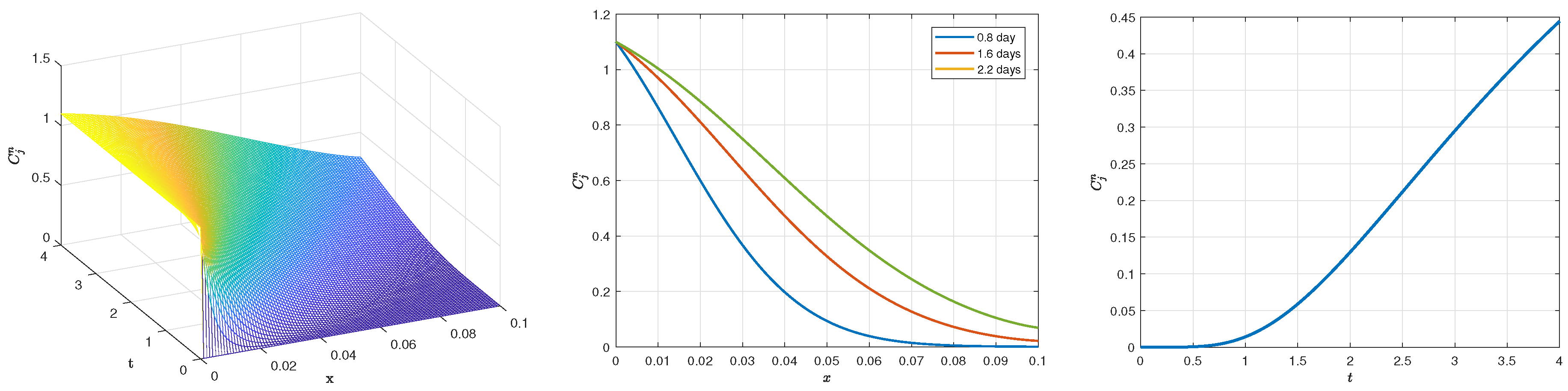
Figure 8.
Numerical simulations obtained with . Left frame: concentration along axial direction at different space and time; Middle frame: the concentration profile of , , and days; Rigth ram: profile at point of the bed.
Figure 8.
Numerical simulations obtained with . Left frame: concentration along axial direction at different space and time; Middle frame: the concentration profile of , , and days; Rigth ram: profile at point of the bed.

© 2020 by the author. Licensee MDPI, Basel, Switzerland. This article is an open access article distributed under the terms and conditions of the Creative Commons Attribution (CC BY) license (http://creativecommons.org/licenses/by/4.0/).
Share and Cite
MDPI and ACS Style
Jannelli, A. Numerical Solutions of Fractional Differential Equations Arising in Engineering Sciences. Mathematics 2020, 8, 215. https://doi.org/10.3390/math8020215
AMA Style
Jannelli A. Numerical Solutions of Fractional Differential Equations Arising in Engineering Sciences. Mathematics. 2020; 8(2):215. https://doi.org/10.3390/math8020215
Chicago/Turabian StyleJannelli, Alessandra. 2020. "Numerical Solutions of Fractional Differential Equations Arising in Engineering Sciences" Mathematics 8, no. 2: 215. https://doi.org/10.3390/math8020215
Note that from the first issue of 2016, this journal uses article numbers instead of page numbers. See further details here.