Finite Element Validation of an Energy Attenuator for the Design of a Formula Student Car

 , , ,
, , ,  and
and 
Abstract
1. Introduction
2. Mathematical Model and Numerical Resolution
2.1. Plasticity
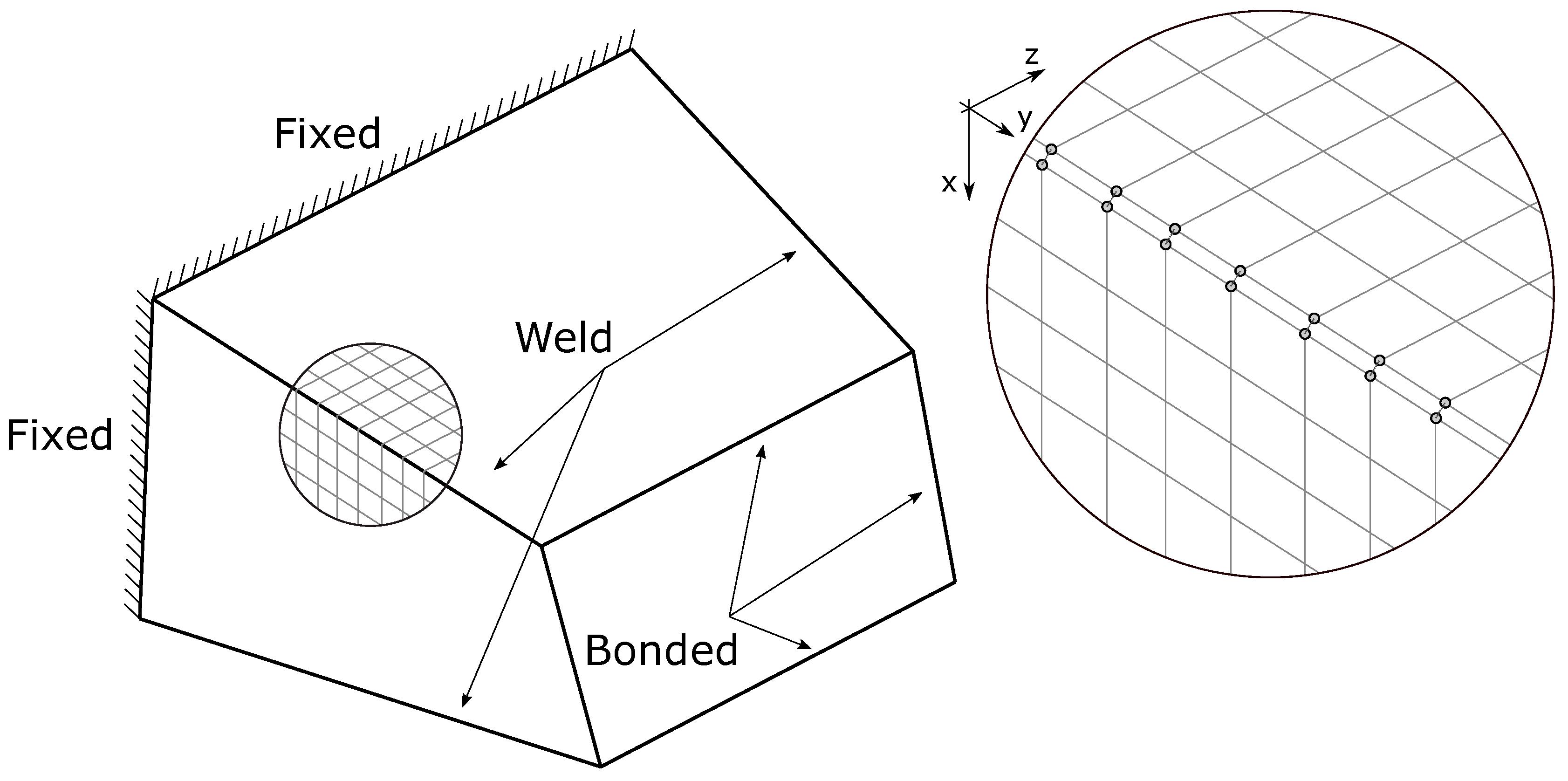
2.2. Weld
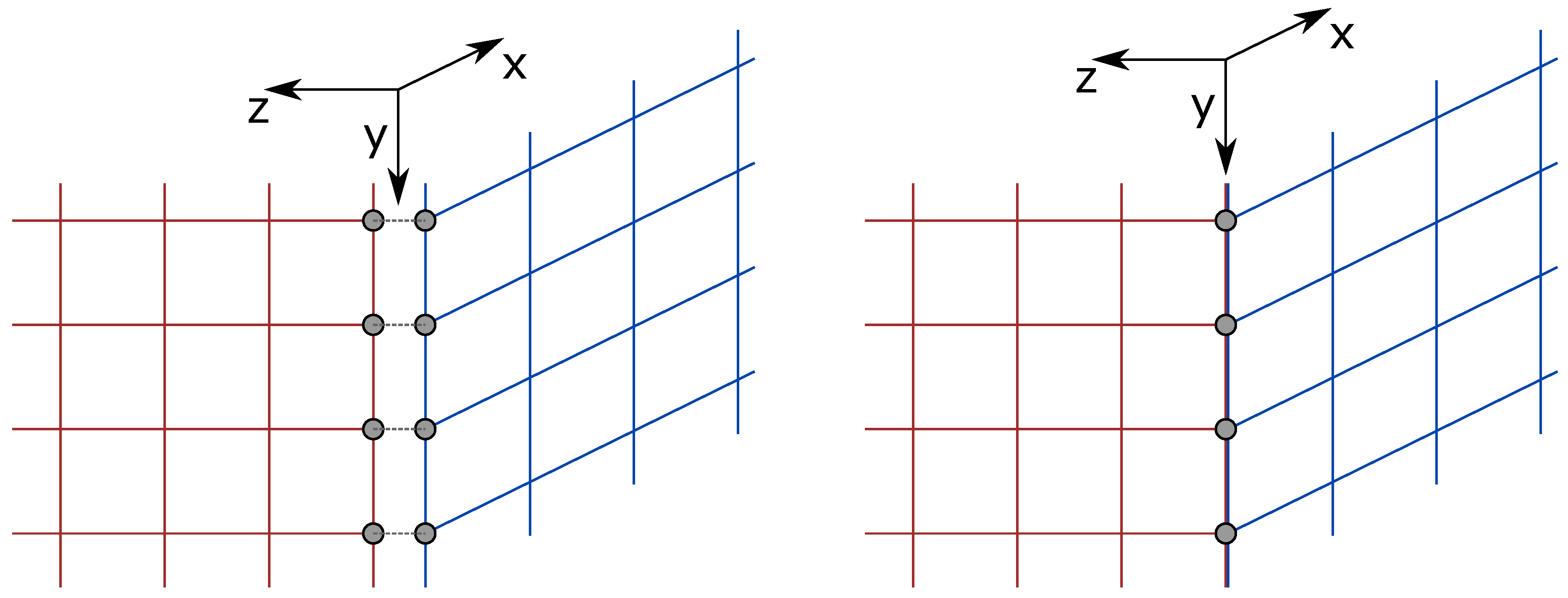
2.3. Spatial Discretization
2.4. Temporal Discretizaton
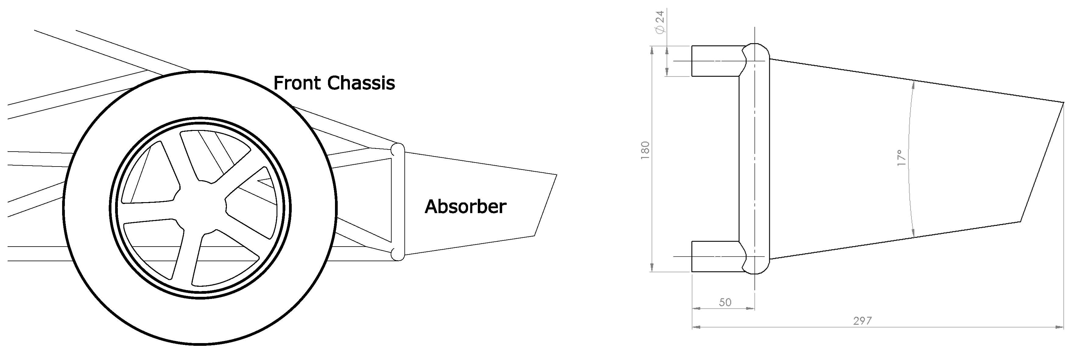
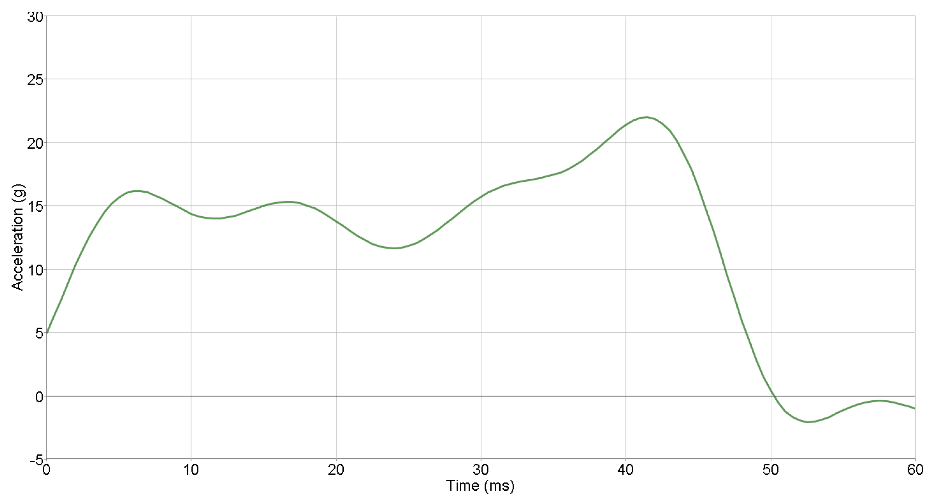
3. Validation Case: Comparison with an Experimental Test
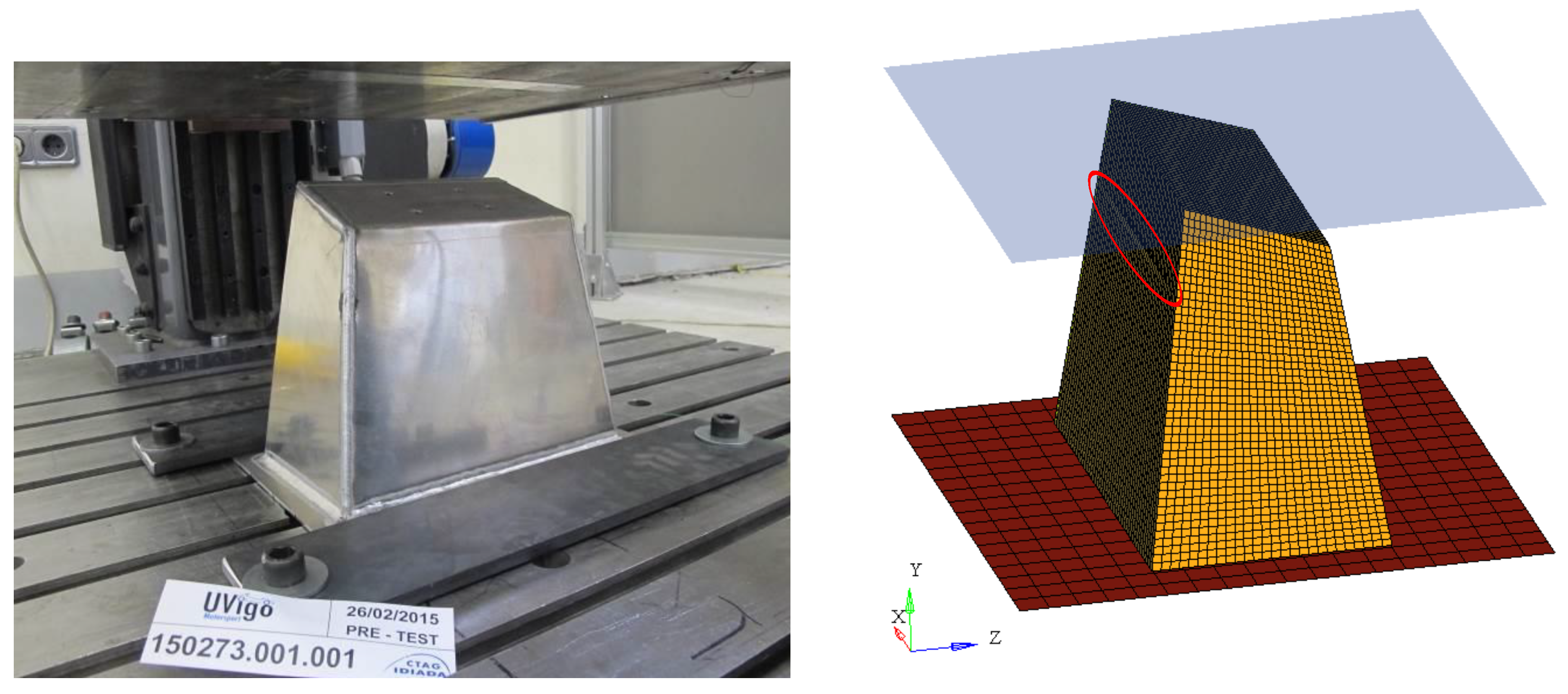
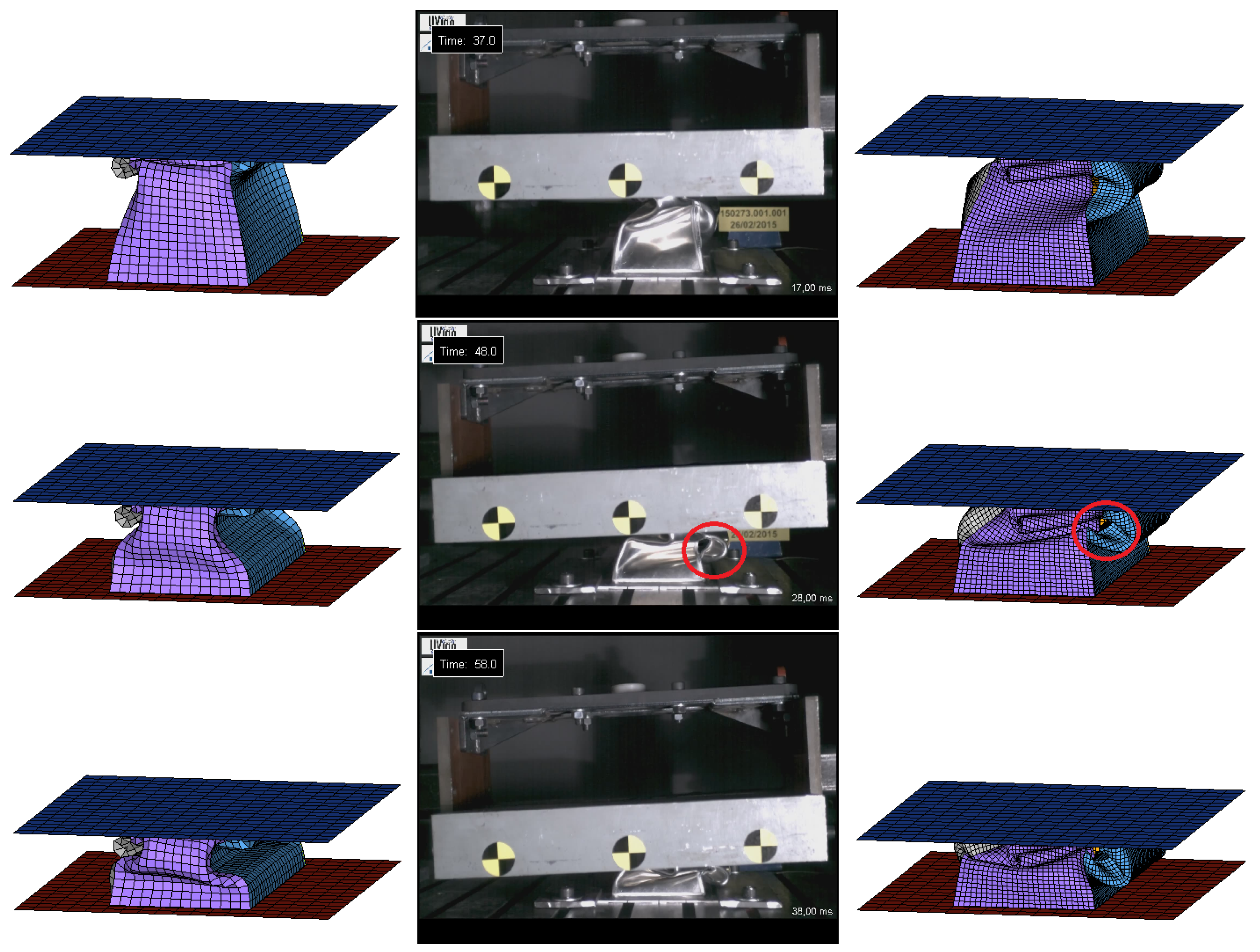
3.1. Real Test
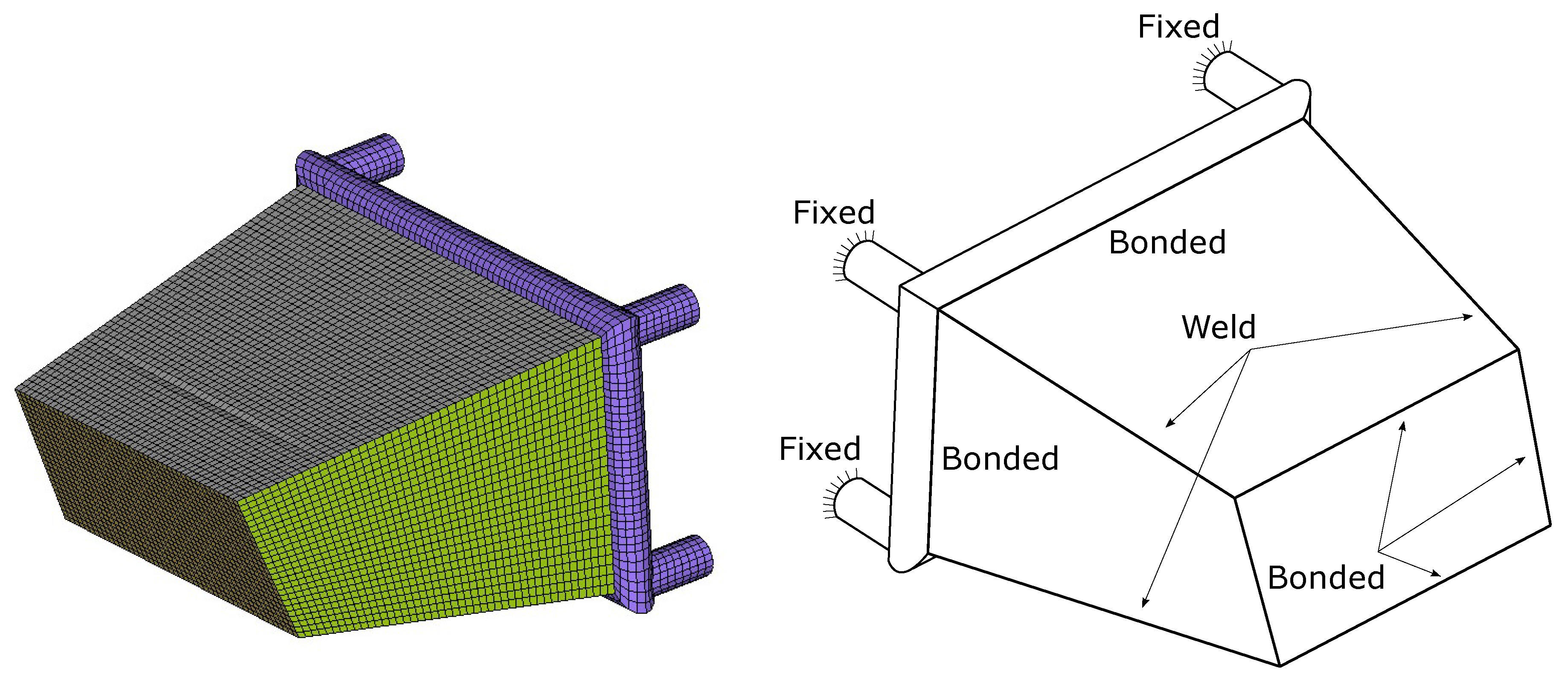
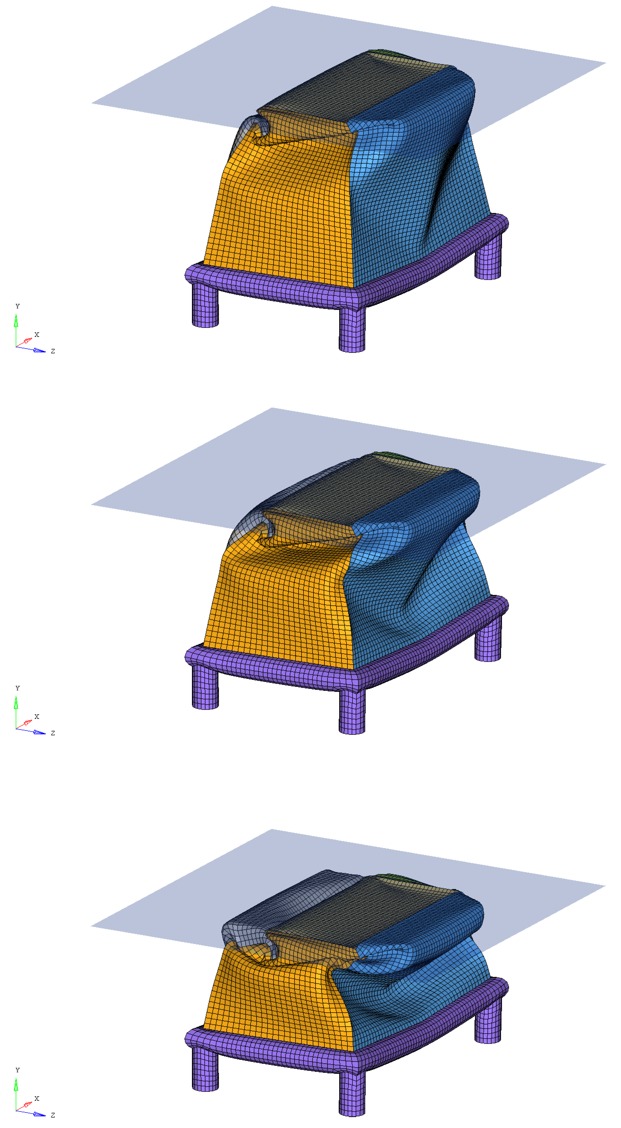
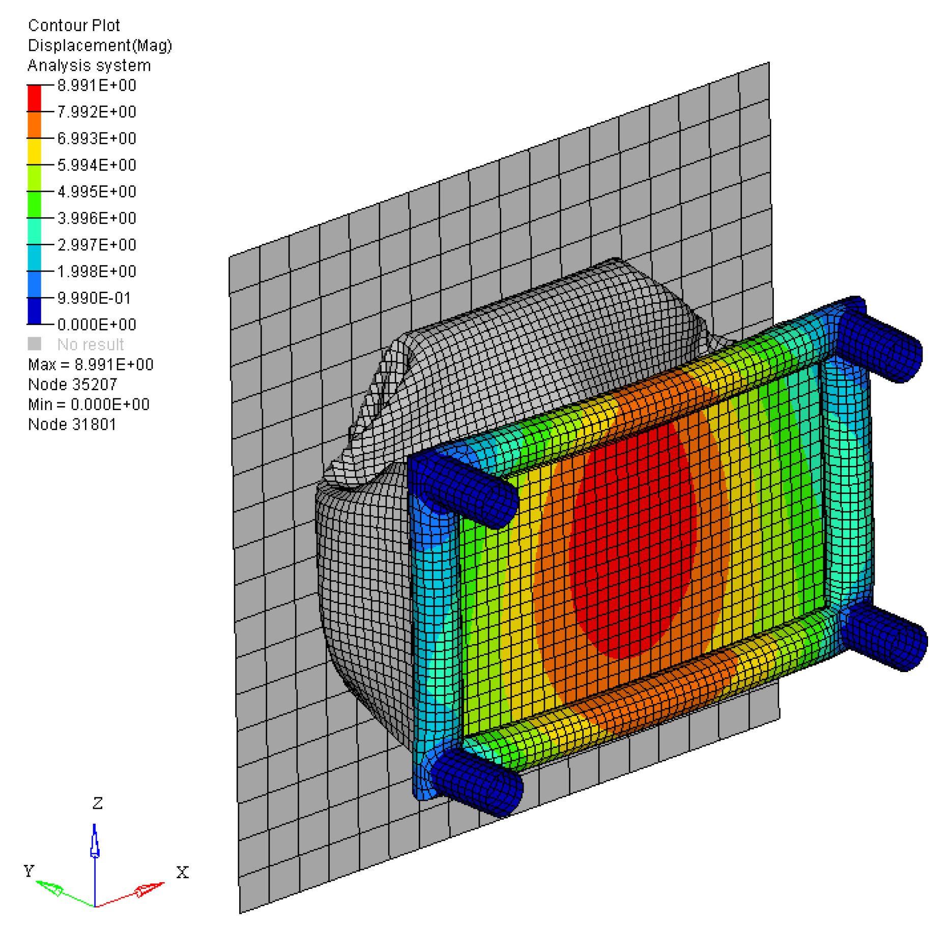
3.2. Finite Element Model
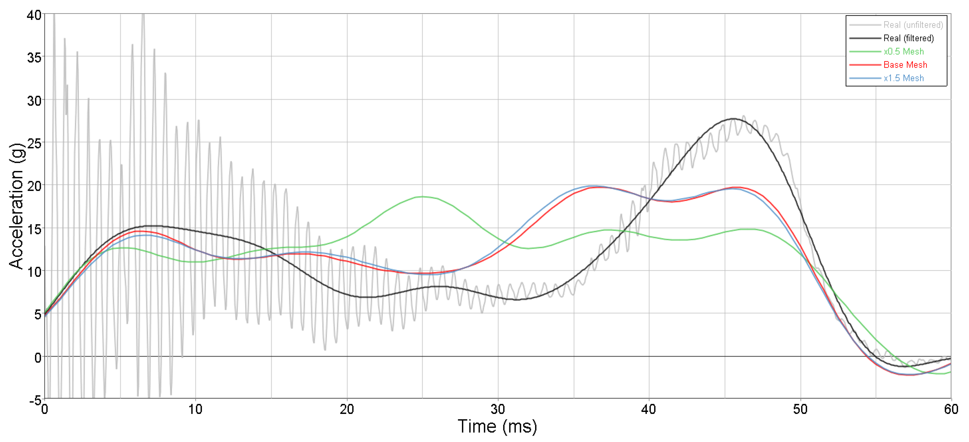
3.3. Results
4. Simulation of the Regulation Case
Results
5. Conclusions
Author Contributions
Funding
Conflicts of Interest
References
- 2018 Formula SAE Rules; SAE International: Warrendale, PA, USA, 2018; Available online: https://www.fsaeonline.com (accessed on 10 March 2018).
- Rooppakhun, S.; Boonporm, P.; Puangcha-um, W. Design and Analysis of Impact Attenuator for Student Formula. SAE Tech. Pap. 2015. [Google Scholar] [CrossRef]
- Mihradi, S.; Golfianto, H.; Mahyuddi, A.I.; Dirgantara, T. Head Injury Analysis of Vehicle Occupant in Frontal Crash Simulation: Case Study of ITB Formula SAE Race Car. J. Eng. Technol. Sci. 2017, 49, 534–545. [Google Scholar] [CrossRef]
- Boria, S. Behaviour of an Impact Attenuator for Formula SAE Car under Dynamic Loading. Int. J. Veh. Struct. Syst. 2010, 2, 45–53. [Google Scholar] [CrossRef]
- Jianhua, W.; Dashuai, X.; Shuai, Z.; Shichao, W. Designing and Experiment study on Front Impact Attenuator for Formula SAE Racecar. Appl. Mech. Mater. 2012, 138–139, 33–37. [Google Scholar]
- Belingardi, G.; Boria, S.; Obradovic, J. Energy Absorbing Sacrificial Structures Made of Composite Materials for Vehicle Crash Design. In Dynamic Failure of Composite and Sandwich Structures; Abrate, S., Castanié, B., Rajapakse, Y., Eds.; Solid Mechanics and Its Applications; Springer: Berlin, Germany, 2013; Volume 192, pp. 577–609. [Google Scholar]
- Yang, Y.; Wu, X.; Terada, S.; Okano, M.; Nakai, A.; Hamada, H. Application of FRP in a vehicle for Student Formula SAE Competition of Japan. Int. J. Crashworth. 2012, 17, 295–307. [Google Scholar] [CrossRef]
- Segade, A.; López-Campos, J.A.; Fernández, J.R.; Casarejos, E.; Vilán, J.A. Finite Element Simulation for Analysing the Design and Testing of an Energy Absorption System. Materials 2016, 9, 660. [Google Scholar] [CrossRef]
- Belingardi, G.; Obradovic, J. Design of the impact attenuator for a formula student racing car: Numerical simulation of the impact crash test. J. Serbian Soc. Comput. 2010, 4, 52–65. [Google Scholar]
- Farlian, R.S.; Ubaidillah Krishna, E.K.; Muhamad, I.F.; Sukmaji, I.C.; Muhamad, H.I. Numerical simulation of several impact attenuator design for a formula student car. AIP Conf. Proc. 2018, 1931, 030036. [Google Scholar]
- Chen, W.; Deng, X. Performance of shell elements in modeling spot-welded joints. Finite Elem. Anal. Des. 2000, 35, 41–57. [Google Scholar] [CrossRef]
- Combescure, A.; Delcroix, F.; Caplain, L.; Espanol, S.; Eliot, P. A finite element to simulate the failure of weld points on impact. Int. J. Impact Eng. 2003, 28, 783–802. [Google Scholar] [CrossRef]
- Langrand, B.; Combescure, A. Non-linear and failure behaviour of spotwelds: A global finite element and experiments in pure and mixed modes I/II. Int. J. Solids Struct. 2004, 41, 6631–6646. [Google Scholar] [CrossRef]
- Matzenmiller, A.; Schweizerhof, K.; Rust, W. Joint failure modeling in crashworthiness analysis. In Proceedings of the Second International LS-DYNA3D Conference, San Francisco, CA, USA, 20–21 September 1994. [Google Scholar]
- Xiang, Y.; Wang, Q.; Fanb, Z.; Fang, H. Optimal crashworthiness design of a spot-welded thin-walled hat section. Finite Elem. Anal. Des. 2006, 42, 846–855. [Google Scholar] [CrossRef]
- Xu, S.; Deng, X. An evaluation of simplified Finite element models for spot-welded joints. Finite Elem. Anal. Des. 2004, 40, 1175–1194. [Google Scholar] [CrossRef]
- Zhang, Y.; Taylor, D. Optimization of spot-welded structures. Finite Elem. Anal. Des. 2001, 37, 1013–1022. [Google Scholar] [CrossRef]
- Langrand, B.; Markiewicz, E. Strain-rate dependence in spot welds: Non-linear behaviour and failure in pure and combined modes I/II. Int. J. Impact Eng. 2010, 37, 792–805. [Google Scholar] [CrossRef]
- Schneider, F.; Jones, N. Influence of spot-weld failure on crushing of thin-walled structural sections. Int. J. Mech. Sci. 2003, 45, 2061–2081. [Google Scholar] [CrossRef]
- Choi, Y.; Kim, J.; Park, Y.W.; Rhee, S. Development of a Spot Weld Analysis Model That Incorporates Strain Rate. Int. Precis. Eng. Manuf. 2012, 13, 245–251. [Google Scholar] [CrossRef]
- Blatnický, M.; Sága, M.; Dižo, J.; Bruna, M. Application of Light Metal Alloy EN AW 6063 to Vehicle Frame Construction with an Innovated Steering Mechanism. Materials 2020, 13, 817. [Google Scholar] [CrossRef]
- Marques, E.S.V.; Silva, F.J.G.; Pereira, A.B. Comparison of Finite Element Methods in Fusion Welding Processes—A Review. Metals 2020, 10, 75. [Google Scholar] [CrossRef]
- Chang, P.H.; Teng, T.L. Numerical and experimental investigations on the residual stresses of the butt-welded joints. Comput. Mater. Sci. 2004, 29, 511–522. [Google Scholar] [CrossRef]
- Anca, A.; Cardona, A.; Risso, J.; Fachinotti, V.D. Finite element modeling of welding processes. Appl. Math. Model. 2011, 35, 688–707. [Google Scholar] [CrossRef]
- Deng, D.; Murakawa, H.; Liang, W. Numerical simulation of welding distortion in large structures. Comput. Methods Appl. Mech. Eng. 2007, 196, 4613–4627. [Google Scholar] [CrossRef]
- Wang, R.; Zhang, J.; Serizawa, H.; Murakawa, H. Study of welding inherent deformations in thin plates based on finite element analysis using interactive substructure method. Mater. Des. 2009, 30, 3474–3481. [Google Scholar] [CrossRef]
- Bucolo, M.; Buscarino, A.; Famoso, C.; Fortuna, L.; Frasca, M. Control of imperfect dynamical systems. Nonlinear Dyn. 2019, 98, 2989–2999. [Google Scholar] [CrossRef]
- López-Campos, J.A.; Segade, A.; Casarejos, E.; Fernández, J.R.; Vilán, J.A. A finite element model to study weld and geometric imperfections in an impact attenuator device. In Proceedings of the IRF2018: 6th International Conference Integrity-Reliability-Failure, Lisbon, Portugal, 22–26 July 2018. [Google Scholar]
- Langseth, M.; Hopperstad, O.S.; Berstad, T. Crashworthiness of aluminium extrusions: Validation of numerical simulation, effect of mass ratio and impact velocity. Int. J. Impact Eng. 1999, 22, 829–854. [Google Scholar] [CrossRef]
- Hirose, S. Shock Absorbing Member. Patent PCT No. PCT/JP2012/070109, 7 February 2014. [Google Scholar]
- Yuen, S.C.K.; Nurick, G.N. The energy-absorbing characteristics of tubular structures with geometric and material modifications: An overview. Appl. Mech. Rev. Trans. ASME 2008, 61, 1–15. [Google Scholar] [CrossRef]
- Stout, M.G.; Rollett, A.D. Large-strain Bauschinger effects in fcc metals and alloys. Metall. Trans. A 1990, 21, 3201–3213. [Google Scholar] [CrossRef]
- Zienkiewicz, O.C.; Taylor, R.L. The Finite Element Method; Butterworth-Heinemann: Oxford, UK, 2000; Volume 2. [Google Scholar]
- Mullen, R.; Belytschko, T. An analysis of an unconditionally stable explicit method. Comput. Struct. 1983, 16, 691–696. [Google Scholar] [CrossRef]
- Mutombo, M. Mechanical properties of 5083 aluminium welds after manual and automatic pulsed gas metal arc welding using E5356 filler. Mater. Sci. Forum 2010, 654–656, 2560–2563. [Google Scholar] [CrossRef]
- Abel, J.F.; Shephard, M.S. An algorithm for multipoint constraints in finite element analysis. Int. J. Numer. Methods Eng. 1979, 14, 464–467. [Google Scholar] [CrossRef]
- Hunêk, I. On a penalty formulation for contact-impact problems. Comput. Struct. 1993, 48, 193–203. [Google Scholar] [CrossRef]
- Zarei, H.R.; Kroger, M. Multiobjective crashworthiness optimization of circular aluminum tubes. Thin-Walled Struct. 2006, 44, 301–308. [Google Scholar] [CrossRef]
- Borvik, T.; Hopperstad, O.S.; Reyes, A.; Langseth, M.; Solomos, G.; Dyngel, T. Empty and foam-filled circular aluminium tubes subjected to axial and oblique quasistatic loading. Int. J. Crashworth. 2003, 8, 481–494. [Google Scholar] [CrossRef]
- Langseth, M.; Hopperstad, O.S.; Hanssen, A.G. Crash behaviour of thin-walled aluminium members. Thin-Walled Struct. 1998, 32, 127–150. [Google Scholar] [CrossRef]
- Yan, W.; Durif, E.; Yamada, Y.; Wen, C. Crushing simulation of foam-filled aluminium tubes. Mater. Trans. 2007, 48, 1901–1906. [Google Scholar] [CrossRef]


| Mechanical Properties | Values |
|---|---|
| Density (kg/m) | 2700 |
| Elastic Modulus (GPa) | 72 |
| Yielding Strength (MPa) | 115 |
| Poisson’s ratio | 0.33 |
| Tangent Modulus (GPa) | 1.082 |
| Mesh | Nodes | Elements | Time |
|---|---|---|---|
| Ref. ×0.5 | 3017 | 2732 | 6 min |
| Reference | 8919 | 8440 | 27 min |
| Ref. ×1.5 | 20,439 | 19,194 | 91 min |
© 2020 by the authors. Licensee MDPI, Basel, Switzerland. This article is an open access article distributed under the terms and conditions of the Creative Commons Attribution (CC BY) license (http://creativecommons.org/licenses/by/4.0/).
Share and Cite
López-Campos, J.A.; Baldonedo, J.; Suárez, S.; Segade, A.; Casarejos, E.; Fernández, J.R. Finite Element Validation of an Energy Attenuator for the Design of a Formula Student Car. Mathematics 2020, 8, 416. https://doi.org/10.3390/math8030416
López-Campos JA, Baldonedo J, Suárez S, Segade A, Casarejos E, Fernández JR. Finite Element Validation of an Energy Attenuator for the Design of a Formula Student Car. Mathematics. 2020; 8(3):416. https://doi.org/10.3390/math8030416
Chicago/Turabian StyleLópez-Campos, José A., Jacobo Baldonedo, Sofía Suárez, Abraham Segade, Enrique Casarejos, and José R. Fernández. 2020. "Finite Element Validation of an Energy Attenuator for the Design of a Formula Student Car" Mathematics 8, no. 3: 416. https://doi.org/10.3390/math8030416
APA StyleLópez-Campos, J. A., Baldonedo, J., Suárez, S., Segade, A., Casarejos, E., & Fernández, J. R. (2020). Finite Element Validation of an Energy Attenuator for the Design of a Formula Student Car. Mathematics, 8(3), 416. https://doi.org/10.3390/math8030416