The intgro-differential equations for each channel in Equation (
12) are solved numerically using the method of successive approximations. Two sets of nodes are chosen on the real and the imaginary axis of the parameter region:
,
and
,
. On each interval
and
the derivatives
and
are assumed to be constant, which allows one to evaluate the integrals in Equations (
6) and (
8) analytically, thus significantly reducing the computational effort. Usually, from 10 to 15 iterations are required to reach the convergence of the iterations with a tolerance of
between successive iterations. The number of the nodes on the upper and the lower side of the channel is chosen to be
and
.
4.1. Cavity Flow with a Fixed Point of Cavity Detachment
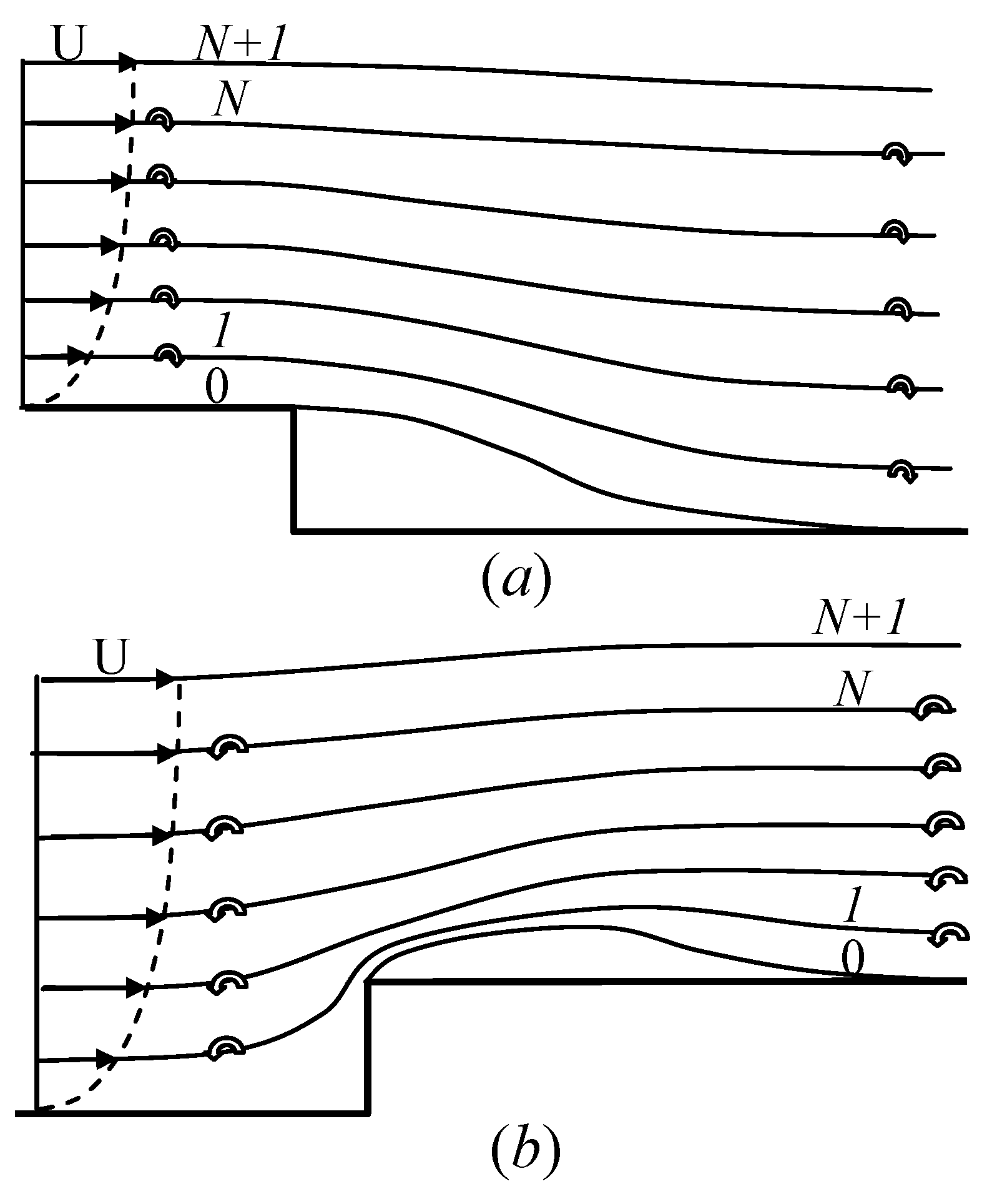
The dimensionless velocity profile in the boundary layer is approximated by the function
where
U is the velocity on the outer boundary of the boundary layer, and
is the boundary layer thickness. The flow rate and the inflow velocity in the channel
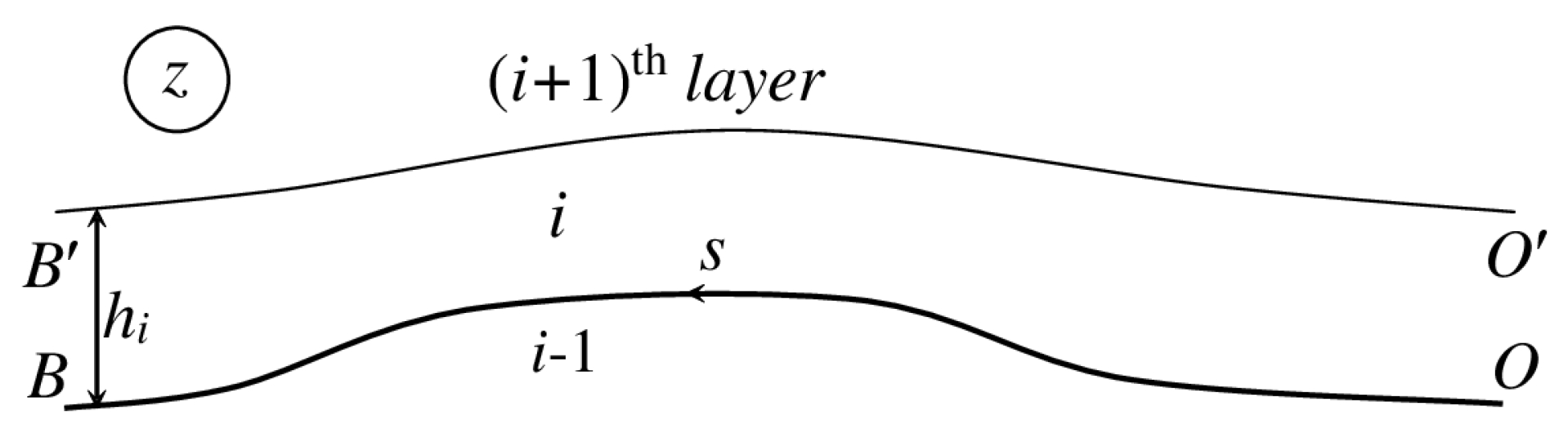
i in view of Equation (
18) are defined as follows
where
is the width of channel
i at infinity
, and
L is the length of the arc
.
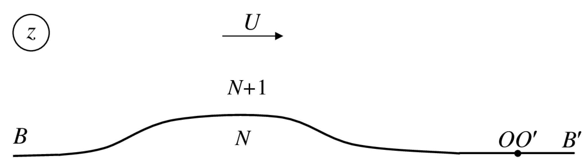
The interaction between adjacent channels accounts for the conditions of velocity direction and pressure continuity across the channel walls.
where
is the slope of the upper side of the channel
,
is the slope of the solid lower side of the channel
i and
,
are the pressures on the upper side of channel
and the lower side of channel
i, respectively.
From the Bernoulli integral for the adjacent channels
we can obtain the relation between the velocity magnitudes on the upper side of channel
and on the lower side of channel
i using Equation (
19),
In the case of a uniform inflow,
and
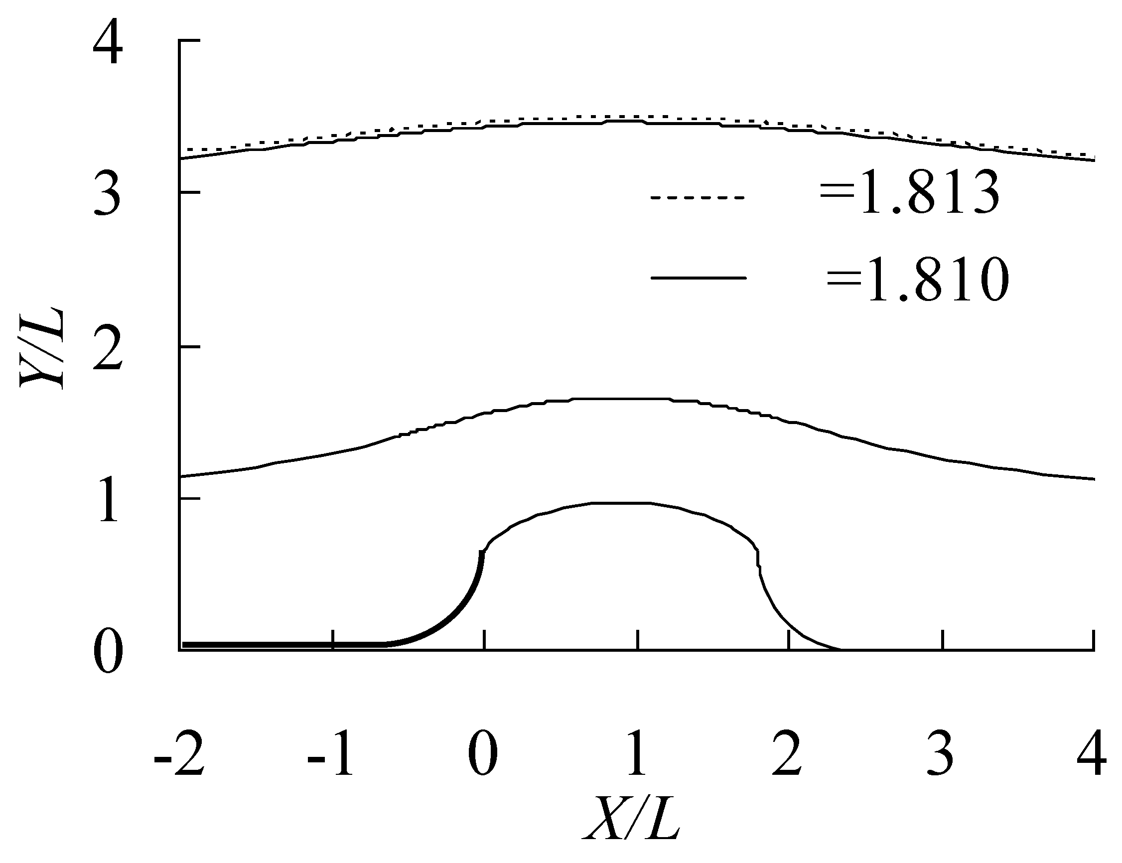
. For the purpose of verification and accuracy estimation of the results, we divide the uniform jet of width
into jets of widths
and
. The cavity length is chosen to be
, and the corresponding cavitation number is determined from the solution.
Figure 5 shows the computed upper boundary of the flow for the two channels (solid line) and for the one channel (dashed line). The obtained cavitation number
for the two channels and
for the one channel demonstrates quite a good accuracy of the method.
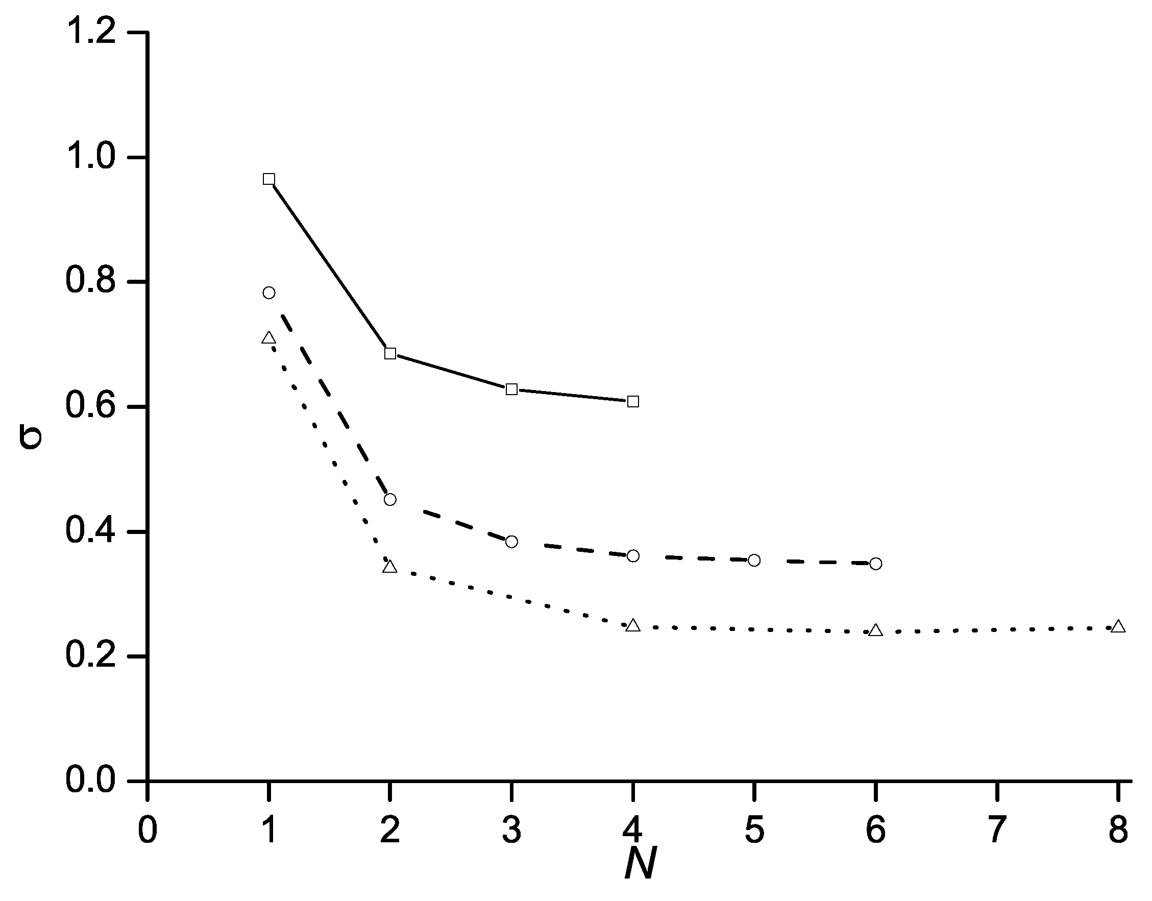
The capability of the method to capture the effect of a nonuniform inflow velocity depends on the required discretization of the boundary layer. As the number of channels increases, the results should converge to those corresponding to the continuous inflow velocity profile.
Figure 6 shows the effect of the number of channels
N on the cavitation number corresponding to cavity length
and a linear velocity profile in the boundary layer. The results show that a 4- or 5-channel discratization of the boundary layer can provide results close to those corresponding to the continuous velocity profile in the boundary layer. It can also be seen that the boundary layer thickness has a weak effect on the required number of discrete channels.
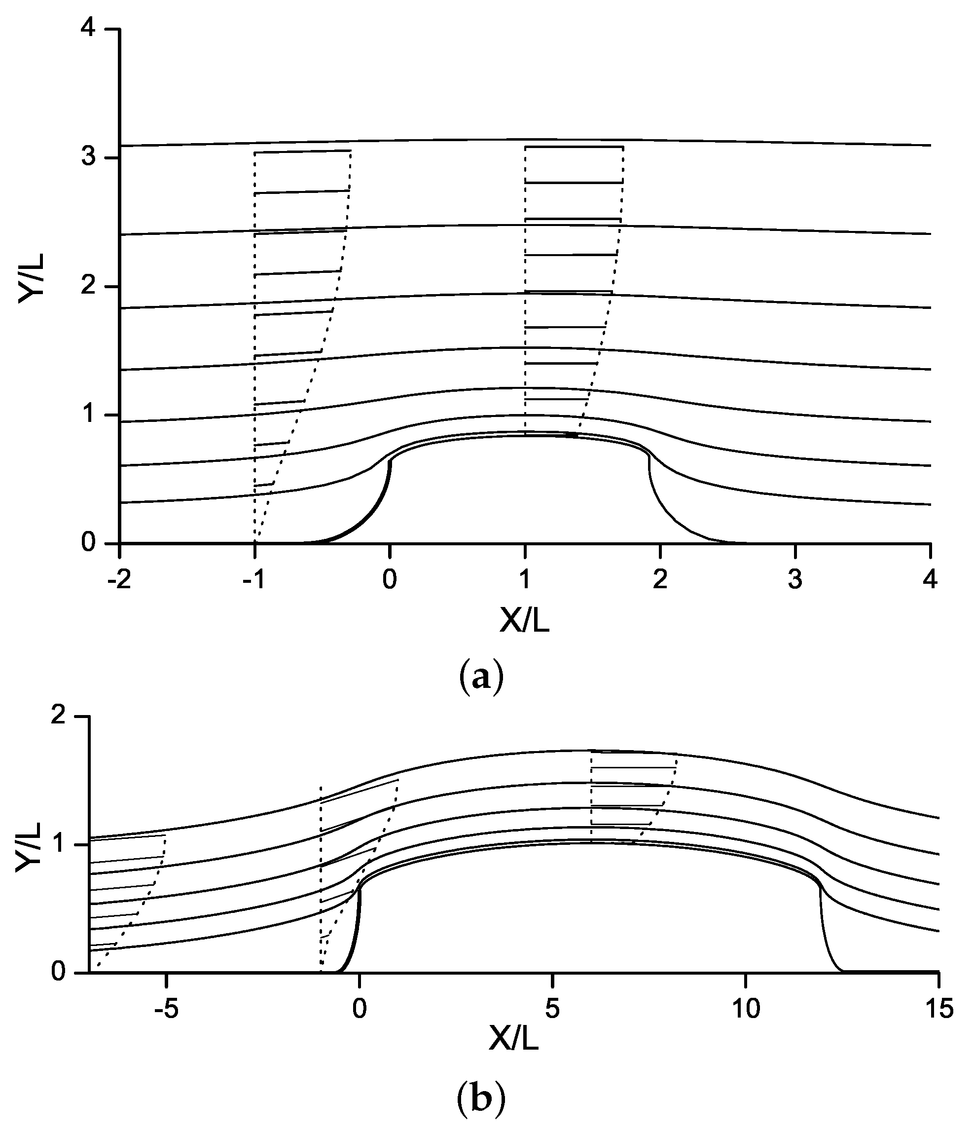
The effect of the boundary layer thickness on the streamline shape and the cavity size is shown in
Figure 7a,b for a parabolic velocity profile (Equation (
18)). It can be seen that the cavity length becomes smaller as the boundary layer thickness increases. This is because the velocity and thus the total flow pressure in the vicinity of the body decrease, which is similar to a greater local cavitation number.
The pressure coefficient can be derived using Equation (
20) relating the outer inviscid flow and channel ‘0’ with the cavity
where
and
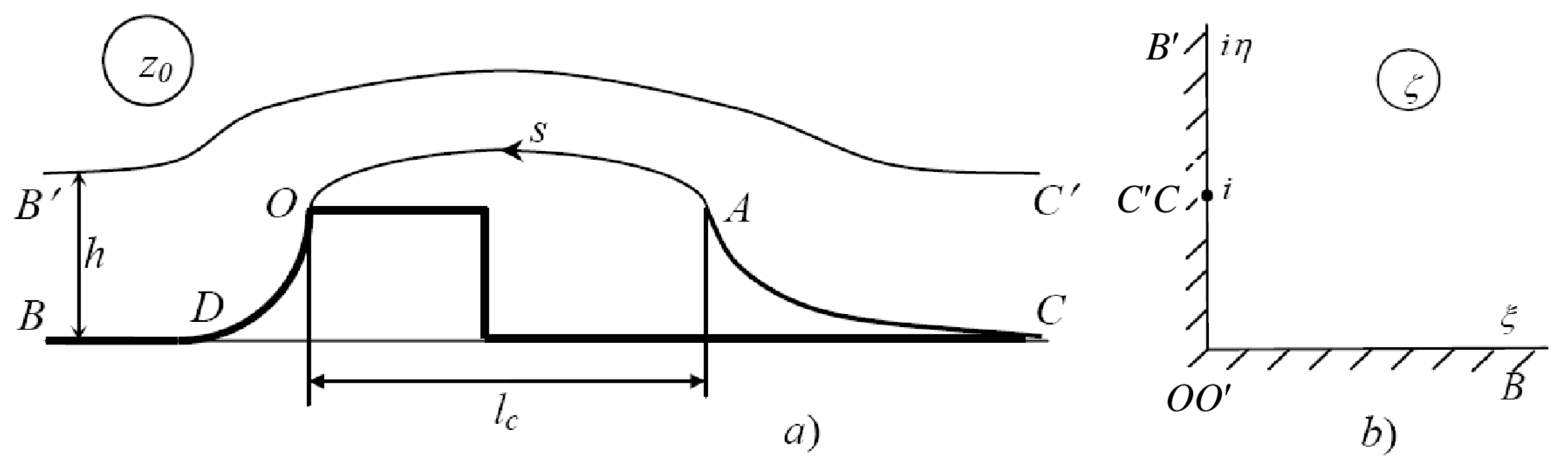
v are the velocity at infinity and on the body in channel ‘0’, respectively. Then, the drag force coefficient is defined as
where the height of the body is
, and
d is the coordinate of point
D on the real axis of the parameter region (see
Figure 2).
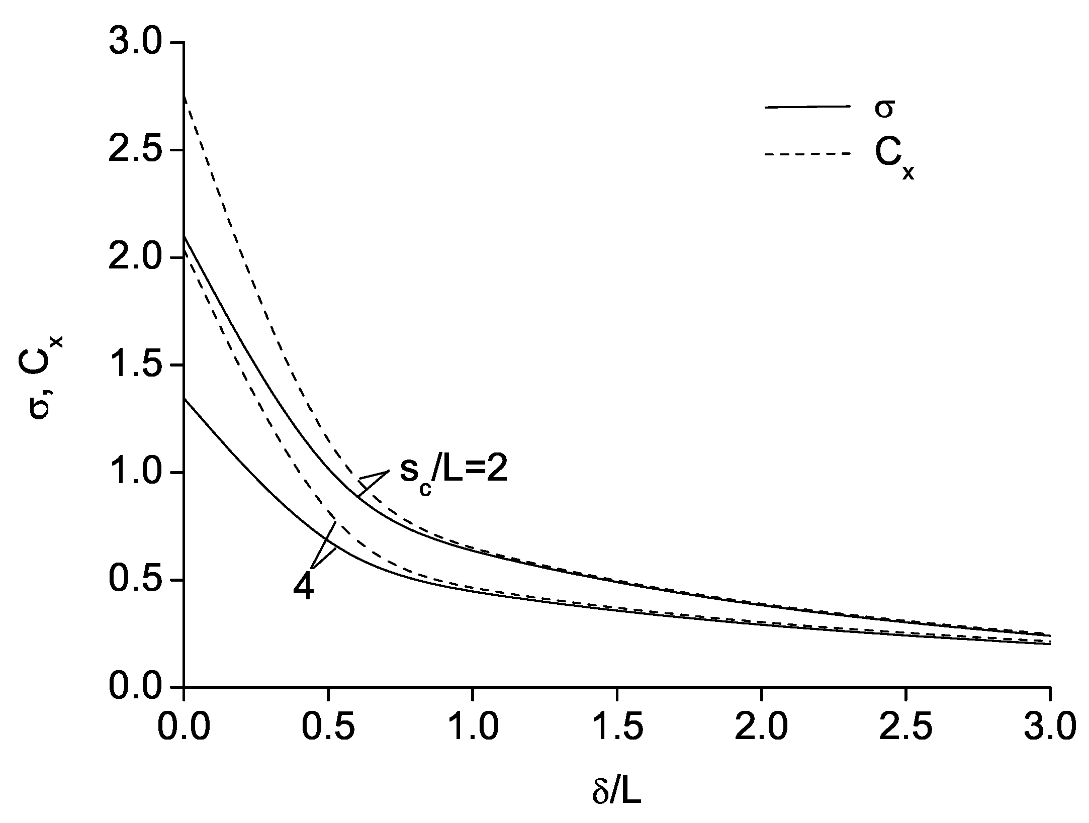
The drag coefficient versus the relative thickness of the boundary layer is shown in
Figure 8. The results correspond to a linear velocity profile of the incoming flow at infinity. It can be seen that for boundary layer thickness
, the cavitation number and the drag coefficient are nearly the same. This is because the contribution of the dynamic component to the total pressure is small. As the boundary layer thickness tends to zero, the cavitation number and the drag coefficient tend to their values corresponding to potential vortex-free flow past the arc of circle.
4.2. Cavity Flow Past a Circular Cylinder
For a body with a sharp edge, the pressure takes its minimal value at the edge, which leads to cavity inception. Therefore, the position of cavity detachment is fixed at that point. For smoothly shaped bodies, the position of the minimal pressure is unknown, and it has to be determined as part of the solution of the problem. In the model of ideal liquid, cavity detachment is determined from Brillouin-Villat’s criterion [
8,
9], which states that the cavity detaches tangentially to the solid surface and the curvature of the free surface is equal to the curvature of the body at the detachment point. These conditions lead to the equation derived by Villat [
9],
where
s is the arc length along the wetted part of the body. The physical meaning of this equation is that the velocity in the flow region reaches its maximal value at the detachment point.
We apply the presented method to the study of the effect of the boundary layer on cavity flow past smoothly shaped bodies. According to the model, the flow in the channels is vortex free, and thus we can use Brillouin-Villat’s criterion [
8,
9] for the zeroth channel, where the cavity occurs. In view of Equation (
6), Equation (
22) takes the form
Equation (
23) determines the position of point
O (
), which influences the function
.
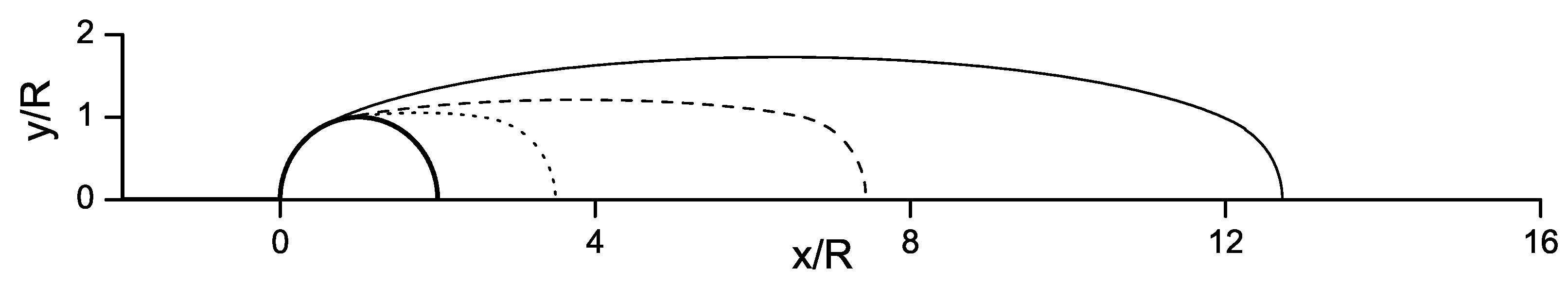
Figure 9 shows cavity contours at different thicknesses of the boundary layer with the velocity profile of (
18). The solid line corresponds to the case without boundary layer. It can be seen that the boundary layer significantly affects the size of the cavity. In addition, the position of the cavity detachment moves somewhat downstream. This feature will be discussed in the following.
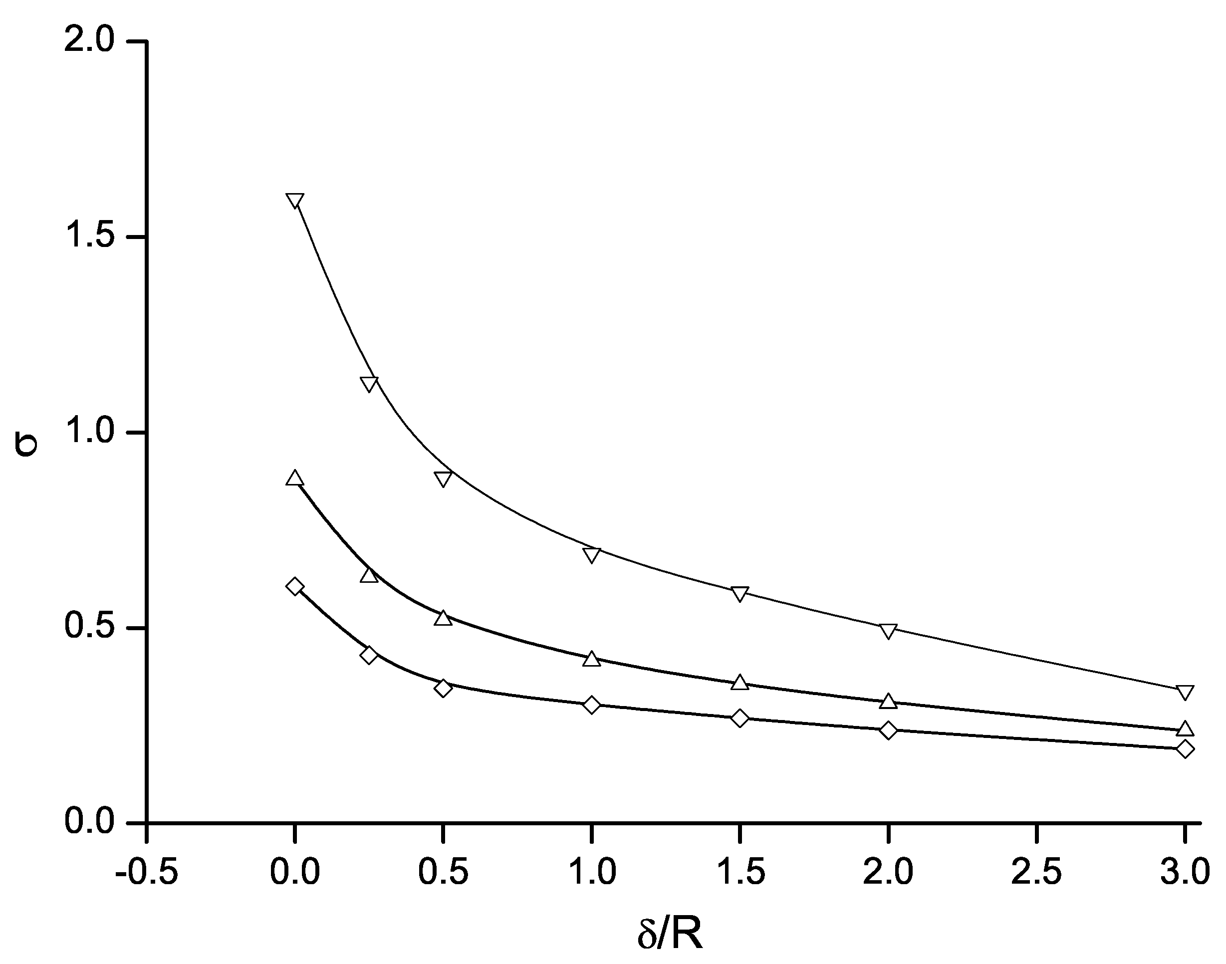
The effect of the boundary layer on the cavitation number is shown in
Figure 10 for different cavity lengths,
. The cylinder radius
R is chosen as the characteristic length. The results are similar to those shown in
Figure 8 for the arc of circle with a fixed position of cavity detachment. The larger the thickness of the boundary layer, the smaller the cavitation number. This implies that a lower pressure at infinity is required to maintain the same cavity size.
Cavity detachment from smooth shaped bodies was studied experimentally by Arakeri and Acosta [
10], Arakeri [
11], Tassin-Leger and Ceccio [
12]. These researches revealed that the real liquid properties such as viscosity, surface tension and the solid/liquid work of adhesion affect the cavity detachment position. Among these physical properties, the liquid viscosity plays the major role due to the development of a boundary layer on the body surface. Arakeri and Acosta [
10] showed that viscous effects are predominant, and the mechanisms of cavity detachment and laminar boundary layer separation are related. A boundary layer separates first and foremost due to an adverse pressure gradient of the external flow, and this determines the cavity detachment position. A recirculation region may occur between the points of laminar boundary layer separation and cavity detachment. Its size may vary significantly depending on the flow configuration, surface tension and the solid/liquid work of adhesion. Sometimes, this region is not observed in experiments [
23].
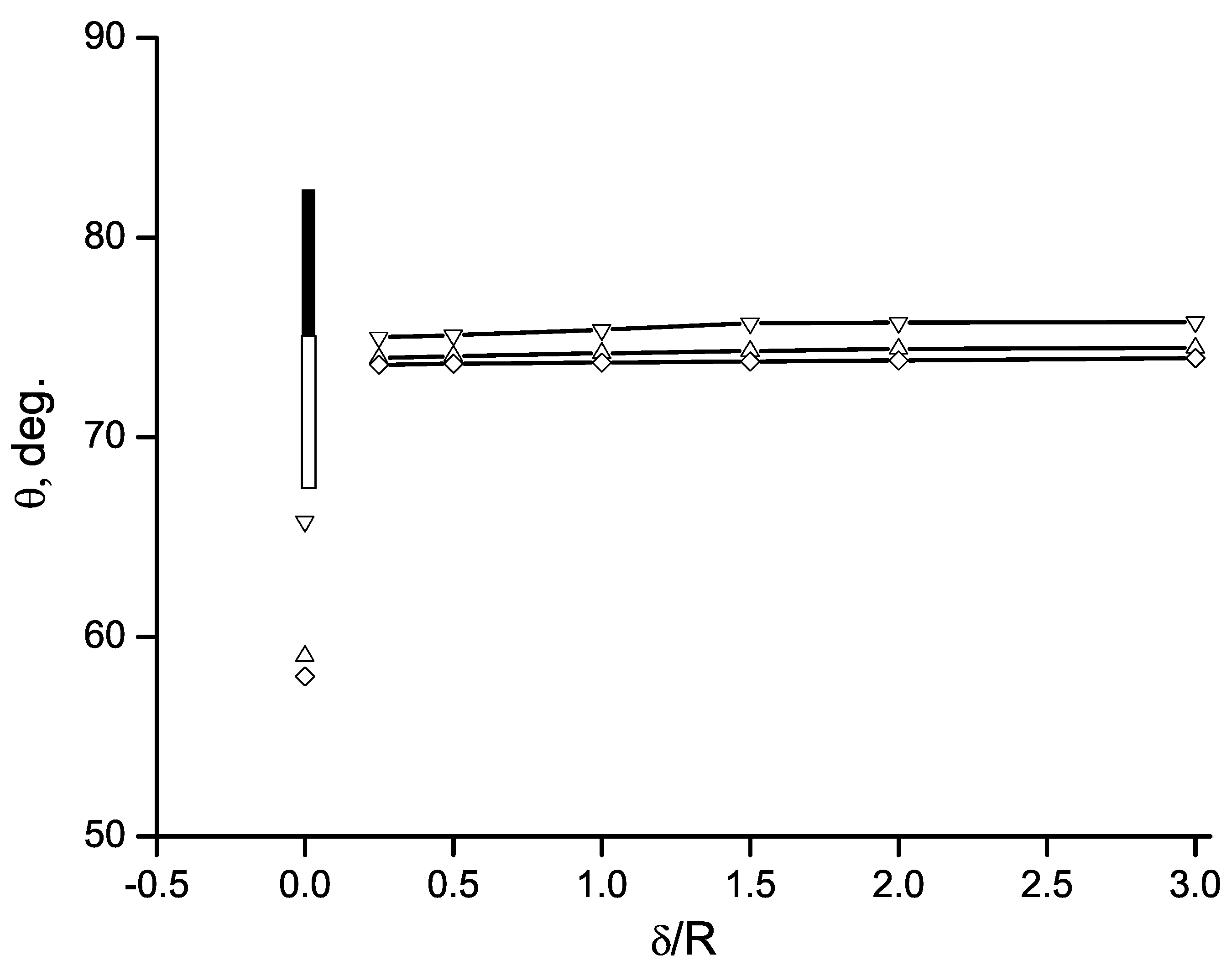
The present model does not account for the flow viscosity, but it can account the effect of the boundary layer, which has been developed at upstream. The angle of cavity detachment,
, measured from the front stagnation point is shown in
Figure 11 as function of the thickness of the boundary layer at upstream,
, for different cavity lengths or the cavitation numbers. The smallest thickness of the boundary layer for which the results were obtained is
. For the smaller thickness of the boundary layer, the larger number of nodes
,
and
,
is necessary to capture the same size of the flow region in the physical plane.
In
Figure 11 it can be seen that the angle
remains nearly constant in the wide range of the boundary layer thickness from
to
. The cavity length, (the cavitation number) also weakly affects the position of cavity detachment. By contrast, the angle
predicted by the model of ideal liquid without a boundary layer,
, is smaller, and it depends on the cavity length. These results are shown as open symbols on the y-axis for different cavity lengths. As the cavity length decreases, the angle
increases, i.e., the position of cavity detachment moves slightly downstream.
The angles
of laminar flow separation and cavity detachment were measured in Tassin-Leger and Ceccio [
12] for a cavitating cylinder in a uniform flow for the range of Reynolds numbers from 6 × 10
to 3 × 10
and for cavitation numbers
and
. There is no upstream boundary layer for this case, i.e.,
. A very thin boundary layer develops on the wetted part of the cylinder surface for this range of Reynolds numbers, which does not affect the outer flow. The angles of laminar separation and cavity detachment measured in those experiments are shown in
Figure 11 as open and solid rectangles, respectively. We note that in those experiments, the position of laminar separation does not depend on the Reynolds number, while the angle of cavity detachment slightly decreases as the Reynolds number increases. Since the boundary layer thickness is very small for the Reynolds numbers in the range mentioned above, it does not affect the outer flow, which determines the pressure gradient along the wetted surface of the cylinder and, accordingly, the separation of the laminar boundary layer.
By comparing the predicted angle of cavity detachment
with the experimental data, we can see that the predicted values of the angle
are in the middle of the range that includes both the separation of the laminar boundary layer and the cavity detachment measured in the experiments. The results obtained can be justified based on the model of ideal liquid, whose results are shown in
Figure 11 as open symbols. The smaller the cavity length (the larger the cavitation number), the larger the angle of cavity detachment. In the presence of a boundary layer, the angle
is governed by the local cavitation number
for the zeroth channel rather than the cavitation number
for the whole flow. As a result that
based on the average velocity
V in the zeroth channel is larger than
based on the velocity
U of the outer inflow, the angle
in the presence of a boundary layer is larger than
without a boundary layer. Although the model developed does not include the physical properties of the liquid directly, the inclusion of the boundary layer into consideration provides relatively good agreement of the cavity detachment with the experimental data.


