Abstract
This study employs exact line search iterative algorithms for solving large scale unconstrained optimization problems in which the direction is a three-term modification of iterative method with two different scaled parameters. The objective of this research is to identify the effectiveness of the new directions both theoretically and numerically. Sufficient descent property and global convergence analysis of the suggested methods are established. For numerical experiment purposes, the methods are compared with the previous well-known three-term iterative method and each method is evaluated over the same set of test problems with different initial points. Numerical results show that the performances of the proposed three-term methods are more efficient and superior to the existing method. These methods could also produce an approximate linear regression equation to solve the regression model. The findings of this study can help better understanding of the applicability of numerical algorithms that can be used in estimating the regression model.
1. Introduction
The steepest descent (SD) method, founded in 1847 by [1], is said to be the simplest gradient and iterative method for minimization of nonlinear optimization problems without constraints. This method is categorized in a single-objective optimization problem which attempts to obtain only one optimal solution [2]. However, due to the low-dimensional property of this method, it converges very slowly. Therefore, since far too little attention has been paid to the modification of the search direction for this method, this study suggests the three-term direction to solve large-scale unconstrained optimization functions.
The standard SD method for solving unconstrained optimization function is defined as
has the following form of direction
where is a continuous differential function in and . This minimization method has the following iterative form
where is the step size. This study is particularly interested in using exact line search procedures to obtain given by
Throughout this paper, without specification, is used to denote the gradient of at the current iterate point, and to denote the Euclidean norm of vectors. The study will also use as the abbreviation of . The superscript T signifies the transpose.
Line search rules is one of the methods to compute (1) by estimating the direction, and the step size, . Generally, it can be classified into two types, exact line search and inexact line search rules. The inexact line search represents methods known as Armijo [3], Wolfe [4] and Goldstein [5]. Despite the fact that the exact line search is quite slow compared to inexact line search, in recent years, an increasing number of studies adopting the exact line search was discovered due to faster computing powers such as in [6]. This research emphasized the exact line search as we assume that this new era of fast computer processors will give an advantage in using this line search.
The remainder of this study is organized as follows: in Section 2, the evolution of the SD method is discussed while in Section 3, the proposed three-term SD methods with two different scaled parameters and their convergence analysis are presented. Next, numerical results of the proposed methods are illustrated and discussed in Section 4 while in Section 5, the implementation in regression analysis of all proposed methods is demonstrated. A brief conclusion and some future recommendations are provided in the last section of this paper.
2. Evolution of Steepest Descent Method
The issue on search direction modification for SD method has grown importance in light of recent as in 2018, [7] introduced a new descent method that used a three-step discretization method which has an intermediate step between the initial point, x0 to the next iterate point, . In 2016, [8] proposed a search direction of the SD method that possessed global convergence properties. The search direction of the proposed, named as ZMRI taken by the name of the researches Zubai’ah, Mustafa, Rivaie and Ismail, has improved the behavior of the SD method where a proportion of previous search directions is added to the current negative gradient. This search direction is given by
The numerical result of the method revealed that ZMRI has superior performance compared to the standard SD and the method was also 11 times faster than SD.
Recently, inspired by (3), [9] proposed a scaled SD method that also satisfied global convergence properties. The search direction is known as which abbreviated from the researcher’s name Rashidah, Rivaie and Mustafa, is given by
The value of was taken from the coefficient in [10] and defined as
where . The method was then compared with standard SD and (3). The results showed that RRM is the fastest solver for about 76.79% of the 14 selected test problems and solved 100% of the problem.
Several modifications to the SD method have been made. Recently, [11] presented a three-term iterative method for unconstrained optimization problems motivated from [12,13,14] defined as follows:
where
As researchers can see, the author put a restart feature that directly addresses the jamming problem. When the step is too small, then the factor approaches the zero vector. The author has also proven that the method is globally convergent under standard Armijo-type line search and modified Armijo-type line search. As a result, the numerical experiments for the proposed method is much better than the methods in [12,13,14].
3. Algorithm and Convergence Analysis of New Three-Term Search Direction
This section presents the new three-term search direction for SD method to solve large-scale unconstrained optimization problems. This research highlights the development of SD method that can lessen the number of iterations and CPU time while establishing the theoretical proofs under exact line searches. Motivated by the above evolutions on SD, the new direction formula is obtained as follows:
In this research, by employing the parameter from the conjugate gradient method which is said to have faster convergence and lower memory requirements [15], two different scaled parameters, and , are presented. For the first direction, the parameters are called as three-term SD and abbreviated as TTSD1 are
while the second direction known as TTSD2 which is an extension of TTSD1, the parameters are
The idea of the extension arises from the recent literature reviews, for instance in [16,17,18,19,20], which seek to improve the performance and effectiveness of the existing methods. The proposed directions with the exact line search procedure were implemented in the algorithm as follows.
| Algorithm 1: Steepest Descent Method. |
| Step 0: Given a starting or initial point , set . Step 1: Determine the direction, using (5). Step 2: Evaluate step length or step size, using exact line search as in (2). Step 3: Update new point, for . If , then, stop, else go to Step 1. |
3.1. Convergence Analysis
This section indicates the theoretical prove that (5) holds the convergence analysis both in sufficient descent directions and global convergence properties.
3.1.1. Sufficient Descent Conditions
Let sequence and be generated by (5) and (1), then
Theorem 1.
Consider the three-term search direction given by (5) with the TTSD1 as scaled parameters and the step size determined by the exact procedure (2). Then condition (6) holds for all.
Proof.
Obviously, if , then the conclusion is true.
Then, to show that for , condition (6) will also hold true.
Multiply (5) by and by noting that for exact line search procedure, we will get
Therefore, condition (6) holds and thus the proof is complete, which implies that is a sufficient descent direction.□
3.1.2. Global Convergence
The following assumptions and lemma are needed in the analysis of the global convergence of SD methods.
Assumption 1.
The level set
is bounded where
is the initial point.
In some neighborhoods
of
, the objective function is continuously differentiable, and its gradient is Lipchitz continuous, namely, there exists a constant such that for any
.
These assumptions yield the following Lemma 1.
Lemma 1.
Suppose that Assumption 1 holds true. Let
be generated by Algorithm 1,
satisfies (6) and
satisfies exact minimization rule, then there exists a positive constant
such that
and one can also have,
This property is known as Zoutendijk condition. Details of this condition are given in [21].
Theorem 2.
Assume that Assumption 1 holds true. Consider
generated by Algorithm 1 above,
is calculated using exact line search and possesses the sufficient descent condition. Then,
Proof.
The proof is done using a contradiction rule. By assuming that Theorem 2 is not true, that is, . Then, there exists a positive constant , such that for all value of . From Assumption 1, we know that there exists a positive constant such that for all values of . From (5) and using the first scaled parameters (TTSD1), we have
The above inequality implies
Thus, from (7), it follows that
which contradicts Zoutendijk condition in Lemma 1.
Therefore,
Hence, the proof is complete. □
Remark 1.
The sufficient property and global convergence for TTSD2 can also be proven similar to the proof of Theorem 1 and 2.
4. Numerical Experiments
This section examines the feasibility and effectiveness of Algorithm 1 with the use of (4) and (5) as the search direction in Step 3 under the exact line search rules by implementing the performance profile introduced by [22] as a tool for comparison. The test problems with the sources are listed in Table 1. The codes were written in MATLAB 2017a.

Table 1.
List of test functions.
For the purpose of comparison, the methods were evaluated over the same set of test problems (see Table 1). The total number of test problems was twenty-six with three different initial points ranging from 2 to 5000 number of variables. The results were divided into two groups, which in the first group was the comparison between the proposed directions with standard and previous SD methods, [8,9] while in the second group the numerical results were compared with another three-term iterative method introduced by [11] using exact line search procedures. Numerical results were compared based on the number of iterations and CPU times evaluated. In the experiments, the termination condition is . We also forced the routine to stop if the total number of iteration exceeded 10,000.
For the methods being analyzed, a performance profile introduced by [22] was implemented to compare the performance of the set solvers S on a test set of problems P. Assuming as number of solvers and as number of problems, they defined .
The performance ratio used to compare the performance by solver s with the best performance by any solver on problem p which they defined as
In order to get the overall evaluations of the solver’s performance, they definedas ρs(t) as a probability for a solver that was within a factor of the best possible ration. The probability is described as
in which the function was the cumulative distribution function for the performance ratio. The performance profile was for a solver was piecewise non-decreasing and continuous from the right at each breakpoint. Generally, the higher value of or in other words, the solver whose performance profile plot is on the top right will win the rest of the solvers or represents the best solver.
Figure 1 show the comparison of the proposed method with the standard SD, ZMRI and RRM methods. In Figure 2 in order to emphasize the proposed search direction from the direction in [11] abbreviated as WH, it might call the present formula as first and second three-term SD methods, TTSD1 and TTSD2, respectively. The performance for all the methods, referring to the number of iterations evaluated and central processing unit (CPU) time, respectively, are displayed.
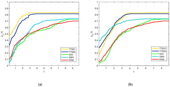
Figure 1.
Performance profile using exact line search procedures between steepest descent (SD) methods based on the (a) number of iterations evaluation; (b) CPU time.
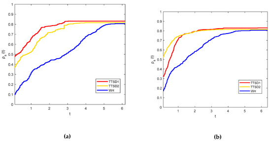
Figure 2.
Performance profile using exact line search procedures between three-term iterative methods based on the (a) number of iterations evaluation; (b) CPU time.
From the above figures, the TTSD1 method outperforms the other methods in both the number of iterations and CPU time evaluations. This can be seen from the left side of Figure 1 and Figure 2 in which TTSD1 is the fastest method in solving all of the test problems and from the right side of the figures, this method also gives the highest percentage of successfully solved test problems compared to other methods. The probability of all the solvers or the methods involved was not approaching 1 which means that they are not able to solve all of the problems tested. The percentage of the successful problems solved by each solver is tabularized in Table 2. Table 2 also presents the CPU time per single iteration based on the evaluation of the total iterations and total CPU times. Although the performance of other methods seems to be much better than the proposed method, TTSD1 and TTSD2 can be considered as the superior method since it can solve 81.02% and 82.97% of the functions tested.
Table 2.
CPU time (in seconds) per single iteration and successful percentage in solving all the functions using the exact line search.
5. Implementation in the Regression Model
In modern times, optimal mathematical models have become common resources for researchers, for instance, in the construction industry, these tools are used to find a solution to minimize costs and maximize profits [31]. Steepest descent method is said to have various applications mostly in finance, network analysis and physics as it is easy to use. One of the most frequent employment of this method is in regression analysis. This paper aims to investigate the use of the proposed direction in describing the relationship between fin dorsal length and the total length of silky shark. The data were collected by [32] from March 2018 to February 2019 at Tanjung Luar Fish Landing Post, West Nusa Tenggara. The study was carried out to set the minimum size of fin products for international trade and the author also pointed out that this data can be used by the fisheries authority to determine the allowed minimum size of silky shark fins for export.
Figure 3 shows the linear approximation between the total length and the length of a dorsal fin of silky shark as . In order to measure the model performance, the coefficient of determination, , has been calculated as a standard metric for model errors and it showed that the value of is close to 1, means there is a strong relationship between the total length of silky shark with the length of its dorsal fin. The total length of the silky shark was measured from the anterior tip of the snout to the posterior part of the caudal fin while the dorsal fin length measured from the fin base to the tip of the fin as shown in Figure 4.
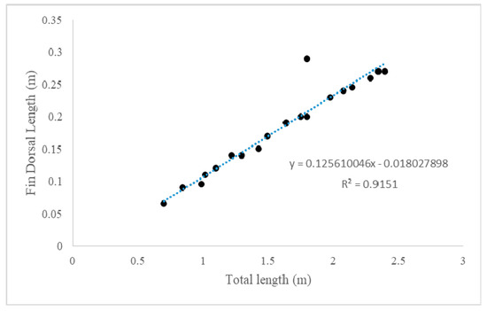
Figure 3.
Relationship of dorsal fin length and the total length of silky sharks.
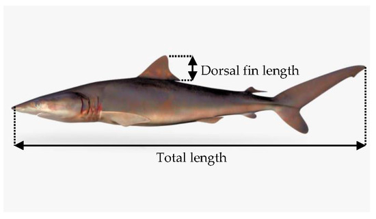
Figure 4.
Silky shark (Carcharhinus falciformis).
The linear regression analysis was implemented by using the dorsal fin length as dependent variables and the total length of a silky shark as an independent variable with a model is indicated as
In order to estimate the above linear regression equation, the least square method was conducted by assuming the estimators are the values of parameters which minimize the objective function as follows:
The sum squares of can be minimized by utilizing the concept of calculus, differentiating (8) with respect to all the parameters involved. The equations can be written in a matrix form and lead to the system of the linear equation. By using the inversion of the matrix method to solve the system of linear equation, the solution is derived as
Another method to find the solution of a system of linear equation is by using the numerical method. In this context, the proposed three-term method is implemented as a numerical method to solve the system as a comparison with the aforementioned inversion of the matrix. To test the efficiency of the proposed method TTSD1 and TTSD2, Table 3 gives an overview of the estimations model coefficients using an inverse method, TTSD methods and also WH method with the number of iterations (with initial point is ).
Table 3.
Summary of results.
The accuracy and performance of these methods are measured by the sum of relative errors by using the total of the differences between the approximation and the exact values of the data. The sum of relative errors are tabulated in Table 3 where the equation of the relative errors is defined as
where the exact value gained from the actual data and the approximate value is the value obtained by each method involved. From Table 3, it can be observed that TTSD1 has the least value of errors followed by the inversion matrix method and TTSD2 which implies that these two methods are comparable with the direct inverse method.
6. Conclusions and Future Recommendations
The main objective of this paper is to propose a three-term SD method also known as the iterative method with two different scaled parameters. The effectiveness of the method, TTSD1 and TTSD2, were tested by comparing with the previous SD (standard, ZMRI and RRM) and three-term method presented in [13], named the WH method, using the same set of test problems under exact line search algorithms. The proposed method possesses sufficient descent and global convergence properties. Through several tests, the method TTSD1 and TTSD2 really outperform the previous SD and other three-term iterative methods. The reliability of TTSD1 and TTSD2 was found to be consistent with the results obtained by the direct inverse method for the implementation in the regression analysis. This finding shows that the methods are comparable and applicable. There is abundant room for further research on the SD method. In the future, we intend to test this new TTSD1 and TTSD2 using the inexact line search.
Author Contributions
Data curation, S.F.H.; Formal analysis, M.M., M.A.H.I. and M.R.; Methodology, S.F.H.; Supervision, M.M., M.A.H.I. and M.R.; Writing—original draft, S.F.H.; Writing—review & editing, M.M., M.A.H.I. and M.R. All authors have read and agreed to the published version of the manuscript. They contributed significantly to the study.
Funding
The authors gratefully acknowledge financial support by the Malaysia Fundamental Research Grant (FRGS) under the grant number of R/FRGS/A0100/01258A/003/2019/00670.
Conflicts of Interest
The authors declare no conflict of interest.
References
- Cauchy, A.-L. Méthode générale pour la résolution des systèmes d’équations simultanées [Translated: (2010)]. Compte Rendu des S’eances L’Acad’emie des Sci. 1847, 25, 536–538. [Google Scholar]
- Pei, Y.; Yu, Y.; Takagi, H. Search acceleration of evolutionary multi-objective optimization using an estimated convergence point. Mathematics 2019, 7, 129. [Google Scholar] [CrossRef]
- Armijo, L. Minimization of functions having Lipschitz-continuous first partial derivatives. Pac. J. Math. 1966, 16, 1–3. [Google Scholar] [CrossRef]
- Wolfe, P. Convergence Conditions for Ascent Methods. SIAM Rev. 1969, 11, 226–235. [Google Scholar] [CrossRef]
- Goldstein, A. On Steepest Descent. SIAM J. Optim. 1965, 3, 147–151. [Google Scholar]
- Rivaie, M.; Mamat, M.; June, L.W.; Mohd, I. A new class of nonlinear conjugate gradient coefficients with global convergence properties. Appl. Math. Comput. 2012, 218, 11323–11332. [Google Scholar] [CrossRef]
- Torabi, M.; Hosseini, M.M. A new descent algorithm using the three-step discretization method for solving unconstrained optimiz ation problems. Mathematics 2018, 6, 63. [Google Scholar] [CrossRef]
- Zubai’ah, Z.A.; Mamat, M.; Rivaie, M. A New Steepest Descent Method with Global Convergence Properties. AIP Conf. Proc. 2016, 1739, 020070. [Google Scholar]
- Rashidah, J.; Rivaie, M.; Mustafa, M. A New Scaled Steepest Descent Method for Unconstrained Optimization. J. Eng. Appl. Sci. 2018, 6, 5442–5445. [Google Scholar]
- Zhang, L.; Zhou, W.; Li, D. Global convergence of a modified Fletcher–Reeves conjugate gradient method with Armijo-type line search. Numer. Math. 2006, 104, 561–572. [Google Scholar] [CrossRef]
- Qian, W.; Cui, H. A New Method with Sufficient Descent Property for Unconstrained Optimization. Abstr. Appl. Anal. 2014, 2014, 940120. [Google Scholar] [CrossRef]
- Cheng, W. A Two-Term PRP-Based Descent Method. Numer. Funct. Anal. Optim. 2007, 28, 1217–1230. [Google Scholar] [CrossRef]
- Xiao, Y.H.; Zhang, L.M.; Zhou, D. A simple sufficient descent method for unconstrained optimization. Math. Probl. Eng. 2010, 2010, 684705. [Google Scholar]
- Li, Z.; Zhou, W.; Li, D.H. A descent modified Polak–Ribière–Polyak conjugate gradient method and its global convergence. IMA J. Numer. Anal. 2006, 26, 629–640. [Google Scholar]
- Jian, J.; Yang, L.; Jiang, X.; Liu, P.; Liu, M. A spectral conjugate gradient method with descent property. Mathematics 2020, 8, 280. [Google Scholar] [CrossRef]
- Yabe, H.; Takano, M. Global convergence properties of nonlinear conjugate gradient methods with modified secant condition. Comput. Optim. Appl. 2004, 28, 203–225. [Google Scholar] [CrossRef]
- Liu, J.; Jiang, Y. Global convergence of a spectral conjugate gradient method for unconstrained optimization. Abstr. Appl. Anal. 2012, 2012, 758287. [Google Scholar] [CrossRef]
- Rivaie, M.; Mamat, M.; Abashar, A. A new class of nonlinear conjugate gradient coefficients with exact and inexact line searches. Appl. Math. Comp. 2015, 268, 1152–1163. [Google Scholar] [CrossRef]
- Hajar, N.; Mamat, M.; Rivaie, M.; Jusoh, I. A new type of descent conjugate gradient method with exact line search. AIP Conf. Proc. 2016, 1739, 020089. [Google Scholar]
- Zull, N.; Aini, N.; Rivaie, M.; Mamat, M. A new gradient method for solving linear regression model. Int. J. Recent Technol. Eng. 2019, 7, 624–630. [Google Scholar]
- Zoutendijk, G. Some Algorithms Based on the Principle of Feasible Directions. In Nonlinear Programming; Academic Press: Cambridge, MA, USA, 1970; pp. 93–121. [Google Scholar]
- Dolan, E.D.; Moré, J.J. Benchmarking Optimization Software with Performance Profiles. Math. Program. 2002, 91, 201–213. [Google Scholar] [CrossRef]
- Andrei, N. An Unconstrained Optimization Test Functions Collection. Adv. Model. Optim. 2008, 10, 147–161. [Google Scholar]
- Moré, J.J.; Garbow, B.S.; Hillstrom, K.E. Testing Unconstrained Optimization Software. ACM Trans. Math. Softw. 1981, 7, 17–41. [Google Scholar] [CrossRef]
- Mishra, S.K. Performance of Repulsive Particle Swarm Method in Global Optimization of Some Important Test Functions: A Fortran Program. Available online: https://papers.ssrn.com/sol3/papers.cfm?abstract_id=924339 (accessed on 1 April 2020).
- Al-Bayati, A.Y.; Subhi Latif, I. A Modified Super-linear QN-Algorithm for Unconstrained Optimization. Iraqi J. Stat. Sci. 2010, 18, 1–34. [Google Scholar]
- Sum Squares Function. Available online: http://www-optima.amp.i.kyoto-u.ac.jp/member/student/hedar/Hedar_files/TestGO_files/Page674.htm (accessed on 20 February 2019).
- Lavi, A.; Vogl, T.P. Recent Advances in Optimization Techniques; John Wiley and Sons: New York, NY, USA, 1966. [Google Scholar]
- Ali, M.M.; Khompatraporn, C.; Zabinsky, Z.B. A numerical evaluation of several stochastic algorithms on selected continuous global optimization test problems. J. Glob. Optim. 2005, 31, 635–672. [Google Scholar] [CrossRef]
- Jamil, M.; Yang, X.-S. A Literature Survey of Benchmark Functions For Global Optimization Problems. Int. J. Math. Model. Numer. Optim. 2013, 4, 1–47. [Google Scholar]
- Wang, C.N.; Le, T.M.; Nguyen, H.K. Application of optimization to select contractors to develop strategies and policies for the development of transport infrastructure. Mathematics 2019, 7, 98. [Google Scholar] [CrossRef]
- Oktaviyani, S.; Kurniawan, W.; Fahmi, F. Fin Length and Total Length Relationships of Silky Shark Carcharhinus falciformis Landed at Tanjung Luar Fish Landing Port, West Nusa Tenggara, Indonesia. E3S Web Conf. 2020, 147, 02011. [Google Scholar] [CrossRef]


© 2020 by the authors. Licensee MDPI, Basel, Switzerland. This article is an open access article distributed under the terms and conditions of the Creative Commons Attribution (CC BY) license (http://creativecommons.org/licenses/by/4.0/).