Finite Element Solution of the Corona Discharge of Wire-Duct Electrostatic Precipitators at High Temperatures—Numerical Computation and Experimental Verification

Abstract

Global warming is the greatest challenge faced by humankind, and the only way to reduce or totally eliminate its effects is by minimizing CO₂ emissions. Electrostatic precipitators are very useful as a means to reduce emissions from heavy industry factories. This paper aims to examine the performance of wire-duct electrostatic precipitators (WDESP) as affected by high-temperature incoming gases with a varying number of discharge wires while increasing their radius. The precipitator performance is expressed in terms of the corona onset voltage on the stressed wires and the corona current–voltage (I–V) characteristic of the precipitators working with incoming gases at high temperatures. The start of the corona onset voltage on the surface of the discharge wires is calculated for the precipitators under high temperatures based on the standard of the self-repeat of avalanches’ electrons developing on the surface of the stressed wires at high temperatures. For this, calculating the electrostatic field in the precipitators with single- and multi-discharge wires due to the stressed wire with the use of the well-known charge simulation method (CSM) with high-temperature incoming gases is important. The modeling of corona I–V characteristics is adopted using the finite element method (FEM) for single- and multi- (3-, 5-, and 7-) discharge wires of WDESP with high-temperature incoming gases. Additionally, the electrostatic field, potential, and space charge of WDESP are calculated by a simultaneous solution of equations of Poisson, current density, and the continuity current density. A WDESP was set up in the Laboratory of High Voltage Engineering of Czech Technical University (CTU) in Prague, the Czech Republic, to measure the corona onset voltage values and corona I–V characteristics for different WDESP configurations at high temperatures with a varying number of discharge wires while increasing their radius. The calculated values of the corona onset voltage based on CSM and the calculated corona I–V characteristics based on FEM agree reasonably with those measured experimentally with high-temperature WDESP.

1. Introductions

Air pollution is defined as the nearness in the open-air environment of at least one contaminant (pollutants) in amounts and durations that can harm humans, plants, living creatures, or property, (materials) or which negatively affects happiness regarding life or the direction of business [1]. Instances of customary contaminants incorporate sulfur dioxide, nitrogen oxides, carbon monoxide, hydrocarbons, unstable natural mixes, hydrogen sulfide, particulate issue, smoke, and dimness [2]. This rundown of air poisons can be partitioned into toxins that are gases or particulates. Gases, such as sulfur dioxide and nitrogen oxides, display dispersion properties and are typically amorphous liquids that change to fluids or a strong state simply by a consolidated impact of expanded weight and diminished temperature. Particulates are defined as any scattered issue, strong or fluid, in which the individual totals are larger than single small atoms (about 0.2 μm in distance across), yet smaller than around 500 micrometers [3]. Of ongoing consideration is the particulate size equivalent to or under 10 mm, with this size being the scope of concern in relation to potential human wellbeing impacts [4]. As of now, the emphasis is on air toxics (or perilous air contaminations). Air toxics allude to particles that are available in the environment and show conceivably poisonous impacts, not exclusively to people but also to the general biological system [5]. In the 1990, the Clean Air Act Amendments (CAAAs) incorporated 189 explicit synthetic substances into the air toxics class [6]. These synthetic concoctions include the mill mixes of the mechanically balanced air conditions of working environments, and they are also related to quality gauges of outside barometrical conditions. The former definition takes into account the amount of convergence of the contaminant with the climate and its related length or the timeframe of the event. This idea is significant in that contaminations that are available at low fixations for brief timeframe periods can be inconsequential as far as encompassing air quality concerns [7].

Air pollutant sources can be arranged by their source, their number, their spatial dispersion, and their type of discharges [8]. Arrangement by type incorporates normal and synthetic sources. Characteristic air toxin sources incorporate plant specks of dust, wind-blown residue, volcanic emissions, and lightning-produced backwoods fires [9]. Artificial sources incorporate vehicles, mechanical procedures, power plants, civil incinerators, etc. Two central explanations behind the cleaning of gases in industry, especially squander gases, are benefits and security. For instance, benefits may result from the use of impact heater gases for warming and force age; however, polluting influences may be expelled from the gases before they can be adequately scorched. A few polluting influences can be monetarily changed into sulfur, or dissolvable recuperation frameworks can be introduced to recoup important hydrocarbon discharges. The security of the wellbeing and government assistance of people in general, as well as of individuals working in the industry and of property, is another factor motivating the cleaning of gases. The sanctioning of air contamination control guidelines mirrors the worry of governments’ in regard to the safety of their citizens. For instance, squander gases containing poisonous constituents, (for example, arsenic or lead vapor) comprise a genuine risk to the health of both plant administrators and the encompassing populace. Other waste gases, even though not typically jeopardizing wellbeing in the fixations experienced, may destroy plants, harm paintwork and structures, or stain backdrops and draperies, subsequently negatively affecting the aesthetic appeal of the area in which they are emitted [10]. These contemplations are not autonomous. For instance, emanations are additionally firmly identified as much as possible with the level of the cost expected to forestall fixations that can harm the biological system. These emanations refer to the suspended particles or residue of waste gases.

In industrial nations, principles were established to impose some command over the levels of emissions of dull smoke in the environment and, subsequently, to decrease air pollution. Electrostatic precipitation is a productive strategy for cleaning modern gases from those suspended [11]. The fundamental standards administering the activity of electrostatic precipitators are moderately direct and are well described in the literature [11,12]. Customary duct-type precipitators are comprised of various release wires hung vertically between grounded collecting plates. A high negative voltage is applied to the release wires, and negative particles are framed by crown release at the wires. These particles quicken as they approach the gathering plates and charge the particles in their manner. At the point when a charged molecule arrives at the gathering plate, the charge is killed and the molecule is collected.

Table 1. Summary of the literature review of the modeling of wire-duct electrostatic precipitators (WDESP).

Authors	Configuration	Methodology		Results
		Advantages	Disadvantages
Zheng et al., 2018 [13]	Wire-plate ESP	Simulation of corona discharge and particle transport behavior with the particle space charge effect.	Disregard the effect of high temperatures.	Numerical modeling. Simulation.
Ziedan, 2016 [14]	Wire-duct ESP	Using CSM and FEM, study the electric field on each wire separately, using varying wire diameters in one device to equalize the electric field on each wire.	Disregard the effect of high temperatures.	Numerical modeling. Experiments.
Wen et al., 2016 [15]	Guidance-plate-covered ESP	Increasing the collection efficiency of the loaded ESP by particles.	Disregard the effect of high temperatures.	Numerical modeling. Simulation. Experiments.
Lu et al., 2016 [16]	Wire-plate ESP	Modeling the particle charging with gas flow.	Disregard the effect of high temperatures.	Numerical modeling.
Farnoosh et al., 2011 [17]	Spike-plate ESP	Using 3-diminution FEM in the calculation of electric fields and I–V characteristics and measuring results.	Disregard the effect of high temperatures.	Numerical modeling. Experiments.

summarizes a literature review of the modeling of wire-duct electrostatic precipitators (WDESP). It is clear that most research works are focused on numerical modeling, simulation, or/and experiment work, while all these research works disregard the effect of high-temperature incoming gases. This is not right due to all the output gases from heavy factories being at high temperatures, and this is this a research gap.

The main contribution of the current research work is summarized as follows:

• Investigating how the performance of single- and multi- (3-, 5-, and 7-) discharge wires of WDESP is influenced by high-temperature incoming gases with a varying number of discharge wires, as well as its radius.
• The performance of WDESP is expressed in terms of the corona-onset voltage and the corona I–V characteristic of the precipitators.
• Calculating the electrostatic field using the well-known charge simulation method (CSM).
• Modeling of WDESP to calculate the corona I–V characteristic using the finite element method (FEM).
• A set-up of WDESP was performed in the High Voltage Laboratory of Czech Technical University (CTU) in Prague, Czech Republic, to measure the values of the corona-onset voltage and the corona I–V characteristics for different WDESP configurations at high temperatures with a varying number of discharge wires, and its radius.

The rest of this paper is sorted as follows: Section 2: electrostatic field calculation of WDESP at high temperatures; Section 3: corona-onset voltage calculation of WDESP at high temperatures; Section 4: finite element method-based corona current–voltage characteristics of WDESP at high temperatures; Section 5: experimental set-up and techniques; Section 6: results and discussions; Section 7: conclusions and outcomes of this work.

2. Electrostatic Field Calculations of WDESP at High Temperatures

The geometry of the WDESP of single- and multi-discharge wires with a heater is shown in Figure 1. The calculation of the electrostatic field in complex electrode geometries is very hard due to the charge distribution being non-uniform around the stressed discharge wires. To calculate the electrostatic field of WDESP at high temperatures, the charge-simulation method is used (CSM) [18,19]. It is assumed that the precipitator is infinitely long in the Z-direction for simplicity. Additionally, the cross-section of the X-Y plane of one quarter of WDESP is shown in Figure 2. The total number of simulated charges is n and there is symmetry around both x and y axes, Figure 2 reduces the number of unknowns to:

$$n= \left(\frac{m{N}_1+2N_2}{4}\right)$$

(1)

where m is the number of discharge wires (m is odd); N₁ is the number of simulated surface line charges on each discharge wire located at radius r_f, and r_f = f × r_c, (f = 0.5 in the present calculation); r_c is the radius of the discharge wires; N₂ is the number of simulated surface line charges on each plate of the WDESP located outside the plate at a distance from the plate equal to the distance between two adjacent simulation charges (a = b), as shown in Figure 2. To find the unknown simulated charges, Q_{S, J}, j = 1, 2, 3, …, N; boundary points are chosen equal to the number of simulated charges located on the surface of the discharge wires and collecting plates (Figure 2). This should satisfy the boundary conditions: $\varphi =V$ (applied voltage at the stressed discharge wires); $\varphi =0$ (zero at the grounded collecting plates).

At any boundary point ith with coordinates (x_i, y_i), the potential ${\varphi }_i$ can be calculated by the summation of the potential due to all the simulated charges.

$${\varphi }_i= {\displaystyle \sum }_{j=1}^n{P}_{ij}{Q}_{S, j}$$

(2)

$$P_{IJ}=ln\left(\frac{1}{R_1.R_2.R_3.R_4}\right)$$

(3)

where P_ij: potential coefficient; i = 1, 2, 3, ……, n; j = 1, 2, 3, ……, n; coordinates of the jth simulation charge are (x_j, y_j); and

$$R_1=\sqrt{{\left(x_i-x_j\right)}^2+{\left(y_i-y_j\right)}^2};R_2=\sqrt{{\left(x_i+x_j\right)}^2+{\left(y_i-y_j\right)}^2}$$

$$R_3=\sqrt{{\left(x_i+x_j\right)}^2+{\left(y_i+y_j\right)}^2};R_2=\sqrt{{\left(x_i-x_j\right)}^2+{\left(y_i+y_j\right)}^2}$$

The following formula is obtained when the simulated charges and potential values satisfy the boundary conditions at the boundary points:

$$\left[P\right]\left[Q_s\right]=\left[V_b\right]$$

(4)

where [P] is (n × n) the potential coefficient matrix; [Q_s] is (n × 1) the unknown simulation charge matrix; and [V_b] is (n × 1) the potential values of the boundary points matrix. By solving this equation, the unknown simulated charges Q_s are obtained.

To check the solution accuracy, a checkpoint is chosen and located in between two boundary points; the potential values are checked against the applied voltages at the stressed discharge wires and zero at the collecting plates.

When the accuracy is checked, the values of the simulated charges are obtained, and the electrostatic field at any point P(x_p, y_p) can be determined:

$${\xi }_x= \left(\frac{\delta }{2\pi {\epsilon }_o}\right){\displaystyle \sum }_{j=1}^n{Q}_{sj}\left(\left(x_{p }- x_{j }\right)\left(\frac{1}{R_1^2}+\frac{1}{R_4^2}\right)+\left(x_{p }+ x_{j }\right)\left(\frac{1}{R_2^2}+\frac{1}{R_3^2}\right)\right)$$

(5)

$${\xi }_y= \left(\frac{\delta }{2\pi {\epsilon }_o}\right){\displaystyle \sum }_{j=1}^n{Q}_{sj}\left(\left(y_{p }- y_{j }\right)\left(\frac{1}{R_1^2}+\frac{1}{R_4^2}\right)+\left(y_{p }+ y_{j }\right)\left(\frac{1}{R_2^2}+\frac{1}{R_3^2}\right)\right)$$

(6)

where $\delta$ is the ion mobility (m²/s-V). Following the theoretical requirement that mobility is proportional to the mean free path, experiments indicate that mobility is almost inversely proportional to the gas density over a wide range of temperatures and pressures of WDESP, which is expressed as [20]:

$$\delta =\frac{273 {\delta }_o P_a}{T+273}$$

(7)

where ${\delta }_o$ is the mobility at standard conditions (i.e., ${\delta }_o$ = 1 at 0 °C and 1 atm); T is the temperature of WDESP (°C); and P_a is the pressure of WDESP (atm).

The magnitude electrostatic field value at any point P(x_p, y_p), which is the root square of adding the square of Equation (6) to the square of Equation (7), is:

$${\xi }_P=\sqrt{\left({\xi }_x^2+{\xi }_y^2\right)}$$

(8)

Figure 3 shows the steps of the calculation procedure of the electrostatic field in WDESP as adopted in the MATLAB computer program based on the well-known technique of CSM. Starting from choosing the number of charges n on the discharge wires and collecting plates, we then test the accuracy of both with Equations (1)–(4). After that, we calculate the electrostatic field using Equations (5)–(8), taking into account the effect of high temperatures with Equation (7).

3. Corona-Onset Voltage Calculation in WDESP at High Temperatures

It has been entrenched by experiment and calculation that the corona-onset voltage starts at the surfaces of stressed HV wires when their electrostatic field reaches a critical value at the applied voltage at a certain temperature of WDESP [19,21]. When applying a negative high voltage to the discharge wires of the WDESP, the electrostatic field near the stressed wires reaches a sill value of gas ionization due to the collision of electrons. In the direction of the maximum electrostatic field, the primary avalanche starts to evolve far away from the stressed wires. The avalanche develops in the ionization zone, where the ionization coefficient is more than the electron attachment coefficient η [21], Figure 4.

A successor (new) avalanche can be found if only the old avalanche should somehow provide an initiating electron at the corona-onset voltage, perhaps by photoemission, positive particle sway, metastable activity, or field emission. Field discharge is conceivable just at field qualities surpassing 5 × 10⁷ V/m [22]. Electron emanation by positive particle sway is multiple significant degrees less likely than photoemission [23]. Metastable has been accounted for to have an impact about equivalent to that of positive particle sway [24]. Along these lines, just the principal instrument (electron emanation by photons) was considered in deciding the beginning voltage.

At a distance x from the beginning of the avalanche, the total number of electrons N_e(x) is expressed as [19,23,24]:

$$N_e\left(x, T\right)=\exp \left({{\displaystyle \int }}_{r_c}^x\left(\alpha \left(x, T\right)-\eta \left(x, T\right)\right)dx\right)$$

(9)

Both $\alpha \left(x, T\right)\mathrm{and} \eta \left(x, T\right)$ are the ionization and attachments coefficients of the air at x and at the temperature T, which depends on the electrostatic field $\xi ,$ which depends on the self-space field of the avalanches, the temperature of WDESP, and the applied voltages on the discharge wires and collecting plates [23].

At step $\mathsf{\Delta }x$ of the avalanche development, the total number of photons is expressed as:

$$\mathsf{\Delta }n\left(x, T\right)= \mathsf{\Theta }\left(x, T\right).\mathsf{\Delta }x.N_e\left(x, T\right)$$

(10)

where $\mathsf{\Theta }\left(x\right)$ is the photon rate productions, which are expressed as [24]:

$$\mathsf{\Theta }\left(x, T\right)=f.\alpha \left(x, T\right)$$

(11)

Additionally, a few of the produced photons reach the cathode:

$$\mathsf{\Delta } n_f=f\left(T\right).\alpha \left(x, T\right).\mathsf{\Delta }x.N_e\left(x, T\right).g\left(x\right).exp\left(-\mu \left(T\right)x\right)$$

(12)

where $\mu \left(T\right)$: the absorption photon coefficient at temperature T; $g\left(x\right)$: the geometry factor which determines the losses of photons at the collecting plates (Appendix A) [19,24]. The process of growing avalanches is continued until it amounts to the boundary of the ionization zone at x = r_i at $\mu = \alpha$.

A successor (new) avalanche will develop at temperatures above the critical value [19,24]:

$$\begin{gathered} N_e= \left(N_{ph}+N_{th}\right) \ge 1 \\ {N}_{ph}= \left({{\displaystyle \int }}_0^{\left(r_i-r_c\right)}{\gamma }_{ph}\left(T\right) \alpha \left(x, T\right).exp\left({{\displaystyle \int }}_0^x\left(\alpha \left(x, T\right)-\eta \left(x, T\right)\right)dx\right).g\left(x\right).exp\left(-\mu \left(T\right) x\right).dx\right) \\ {N}_{th}= M.T^2.exp\left(\frac{-e.W_n\left(\xi , T\right)}{k.T}\right).S.t \end{gathered}$$

(13)

where $N_{ph}$: the number of photo-emitted electrons from the stressed discharge wires; ${\gamma }_{ph}$: the photon electron emission coefficient; $W_n\left(\xi , T\right)$: the net of the work function of stressed wires at temperature T and space-charge-free field $\xi$; S: the surface area of the stressed discharge wires; t: the time of growth of the first avalanche; e: the charge of the electron; k: Boltzmann’s constant.

The corona-onset voltage V_o is a critical value for the previous relation, Equation (13), because the coefficient values $\alpha \left(x, T\right), \mu \left(x, T\right), \eta \left(x, T\right), \dots .$ are dependent on the corona-onset voltage V_o. The corona-onset voltage V_o is calculated for different directions of avalanche growth around the stressed discharge wire at different values of temperatures of incoming gases. The procedure is repeated to calculate $V_o\left(\psi \right)$ for all the discharge wires in the WDESP. Figure 5 shows the steps of the calculation of the corona-onset voltage in WDESP, as adopted in the MATLAB computer program with high-temperature incoming gases.

4. Finite Element Method-Based Corona Current-Voltage Characteristics of WDESP at High Temperatures

4.1. Governing Equations of the Ionized Field in WDESP

Poisson’s equation, which relates the electric field intensity with the space-charge E and the space-charge density $\rho ,$ is expressed as [25]:

$$\nabla .E= \frac{\rho }{{\epsilon }_0}$$

(14)

where ε_o is the free space permittivity. The current density continuity or the vector of ionic flow J is expressed as:

$$\nabla .J=0$$

(15)

The vector of the ionic flow is a function of the electric field:

$$J=k.\rho .E$$

(16)

where k is the ions’ mobility. The potential scalar with the space-charge $\mathsf{\Phi }$ can be defined as:

$$E= - \nabla .\mathsf{\Phi }$$

(17)

Many trials cited in the literature for the investigation of the ionized fields depend on some rearranging suppositions. The most well-known ones are as per the following: (1) the electrode spacing is filled with unipolar space charge, such as the wires’ polarity. (2) Deutsch’s assumption [26,27]—i.e., the space charge influences just the magnitude and not the direction of the electric field—is expressed as:

$$E= \lambda .\xi$$

(18)

where $\lambda$: the point function scalar of space coordinates contingent upon charge distribution; $\xi$: the space-charge-free field.

(3) The ions’ mobility values are kept constant, (4) we neglect the thermal diffusion effect, and (5) at the corona-onset voltage value, the electrostatic field E_o around the periphery discharge wires is also kept constant.

The discharge wires and collecting plates are long enough along the Z-direction, so Equation (17) in the two-dimensional, X- and Y-coordinate system is expressed as:

$$\frac{{\partial }^2\mathsf{\Phi }}{\partial x^2}+\frac{{\partial }^2\mathsf{\Phi }}{\partial y^2}=-\frac{\rho }{{\epsilon }_o}$$

(19)

4.2. Finite Element-Based Corona Current-Voltage Characteristics of WDESP at High Temperatures

The finite element method (FEM) [25,26,27,28,29,30,31] is adopted to analyze the electric field with the space-charge in WDESP configurations with high-temperature the incoming gases. Deutsch’s assumption and the constant value of field intensity at the surface periphery of the discharge wires can be corrected or eliminated using the FEM technique.

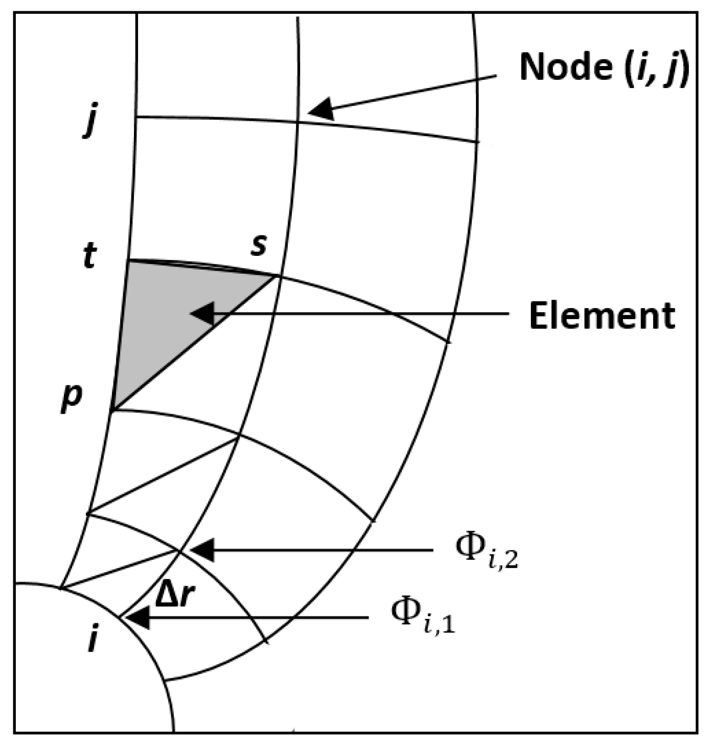
4.2.1. Finite Element Grid

Figure 1 shows the geometry of the WDESP of single- and multi-discharge wires with a heater. The applied voltage V on the stressed discharge wires and the two collecting plates are grounded—i.e., V = 0. It is assumed that the magnitude of the electric field E_o is kept constant at the corona-onset value, but its value is changed from point to point around the wire periphery [25]. The field lines extending between the stressed discharge wires and the collecting plates divide the precipitator volume into flux tubes; among them, the ions conduct from wires to collecting plates (Figure 6). When the field lines intersect with equipotential contours, the finite element grid is generated from the quadrangles, which are divided into two triangle elements [28,29], as shown in Figure 7.

Rewriting Equation (15) using Equation (16), and the current density continuity equation will be expressed as:

$$\nabla .\left(k\rho E\right)=0$$

(20)

During each flux-tube:

$$\frac{d\rho }{dl}\iota =-\frac{{\rho }^2}{{\epsilon }_{o}E}$$

(21)

where $\iota$ is a unit vector which is constant for each flux-tube. To find the space-charge density at all the nodes situated along the axis of the flux-tube, this should be integrated into Equation (21) [29,30].

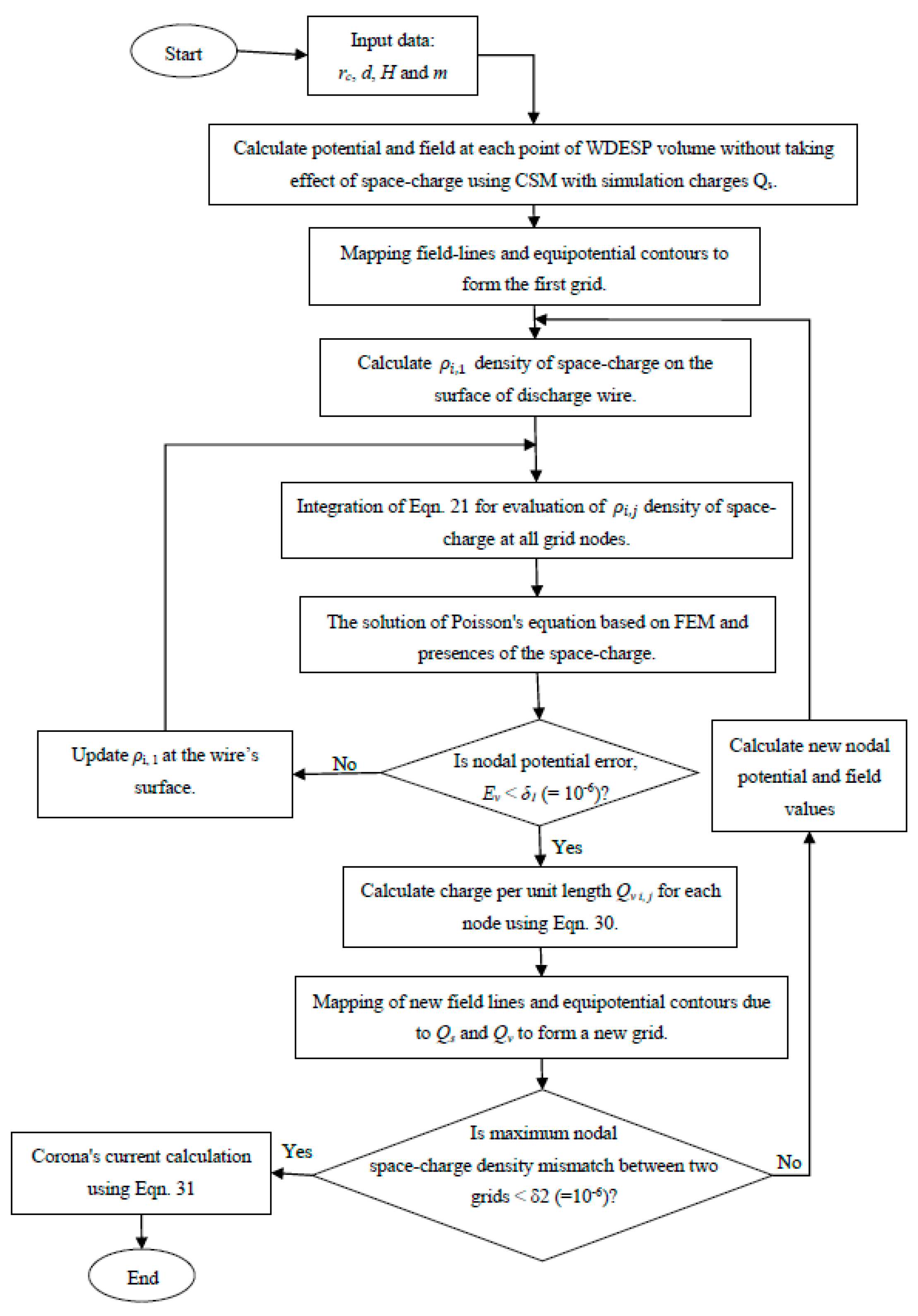
4.2.2. Solution of Poisson’s Equation Using FEM

For each element, the potential ϕ is a linear function of coordinates which is expressed as [29,31,32,33,34]:

$$\mathsf{\Phi }= {\mathsf{\Phi }}^e{W}^e= {\mathsf{\Phi }}_p{W}_p+ {\mathsf{\Phi }}_s{W}_s+{\mathsf{\Phi }}_t{W}_t$$

(22)

where p, s, and t: nodes at element e; W: the corresponding space shape function, as shown in Figure 7. An energy function $R{F}^{\left(e\right)}$ is used to solve Poisson’s equation, which listed in Equation (19) [29,31,32,33,34]:

$$R{F}^{\left(e\right)}=-{{\displaystyle \int }}_A^{ }{\left[W\right]}^T\left[{\left(\frac{\partial \mathsf{\Phi }}{\partial x}\right)}^2+{\left(\frac{\partial \mathsf{\Phi }}{\partial y}\right)}^2+\frac{\rho }{{\epsilon }_o}\right]dA$$

(23)

where A: the area of the triangle element; [W]: the element’s shape function; [W]^T: the transposed [W]. Poisson’s equation is solved to minimize the energy functional $R{F}^{\left(e\right)}$ at the $\rho$ values known at each node, which will give the following equation at the nodes as a function of the potential $\mathsf{\Phi }$:

$$\left[k^e\right]\left[{\mathsf{\Phi }}^e\right]=\left[f^e\right]$$

(24)

where $\left[k^e\right]$: element stiffness matrix; [${\mathsf{\Phi }}^e$]: unknown potentials with the space-charge of the element nodes; [$f^e$]: the free term which entails charge density values at the element nodes, which is calculated for any element as [29,31,32,33,34]:

$$\left[f^e\right]=-\frac{A}{3{\epsilon }_o}\left(\begin{array}{c}{\rho }_p\\ {\rho }_s\\ {\rho }_t\end{array}\right)$$

(25)

where ${\rho }_p$, ${\rho }_s$, and ${\rho }_t$ are the space-charge density at nodes p, s, and t of element e, respectively (Figure 7). A is the per unit length area of the triangle in the Z-direction and is determined as follows:

$$A= \frac{1}{2}\left|\begin{array}{c}1 x_p y_p\\ 1 x_s y_s\\ 1 x_t y_t\end{array}\right|$$

(26)

where (x_i, y_i), i = p, s, and t are the nodal coordinates of element e.

By applying Equation (24) for all the framework components (grid elements):

$$\left[K\right]\left[\mathsf{\Phi }\right]=\left[F\right]$$

(27)

where [K]: stiffness global matrix $= {\displaystyle \sum }_{e=1}^M\left[K^e\right]$; [Φ]: the estimated nodal vector potentials; and [F]: the assembled free-term—$\left[F\right]= {\displaystyle \sum }_{e=1}^M\left[f^e\right]$.

Solving the set (27) determines the array of nodal potential Φ. This is the second gauge of the nodal potentials ${\mathsf{\Phi }}^{\left(2\right)}$ because the space-charge exists. The value of the electric field E₀ at the wire surface is kept constant and is used in the shaping of FE. This is acquired by seeing that $E_0=\left({\mathsf{\Phi }}_{i, 1}-{\mathsf{\Phi }}_{i, 2}\right)/\mathsf{\Delta }{r}_i$, where Δr_i: the radial distance between the first two nodes along the ith flux-tube axis; Δr_i should be smaller than the radius of the discharge wires; ${\mathsf{\Phi }}_{i, 1}$ and ${\mathsf{\Phi }}_{i, 2}$: the potential at nodes (i, 1) and (i, 2) for the ith flux-tube, respectively (Figure 7).

4.2.3. Potential Updating

The error of the nodal potential E_V is calculated based on the comparison between the last two potential estimates at every node, ${\mathsf{\Phi }}^{\left(m\right)}$ and ${\mathsf{\Phi }}^{\left(m+1\right)},$ which are expressed as [30,35,36]:

$$E_V= \frac{{\mathsf{\Phi }}^m-{\mathsf{\Phi }}^{m-1}}{\left({\mathsf{\Phi }}^m+{\mathsf{\Phi }}^{m-1}\right)/2}$$

(28)

If the error of the nodal potential becomes more than an endorsed esteem δ₁, a correction value of ${\rho }_{i,1}$, which is the density of space-charge on the surface of the discharge wires, is expressed as:

$${\rho }_{i,1 new}= {\rho }_{i,1 old} \left[1+\tau .max\left(E_V\right)\right], i=1, 2, 3, \dots , M$$

(29)

where τ: acceleration factor; M: number of flux-lines. Figure 8 shows the flowchart for calculating the corona I–V characteristics based on the FEM.

4.2.4. Grid Updating

The space charges distributed over the precipitator volume are formulated by separating the line-charges at the nodes of the grid. So, at node (i, j), as shown in Figure 9, the charge per unit length $Q_{V i,j}$ is calculated by [37,38]:

$$Q_{V i,j}={\rho }_{i,j} . V_{i,j}$$

(30)

where V_i,j: the volume per unit length; ${\rho }_{i,j}$: the charge-density correction value. At node (i, j), the lines defining the volume are also field lines emanating from the discharge wire surface and terminating at the collecting plate. The volume surrounding each node is defined by the intersection between the field lines and the equipotential contours, as shown in Figure 9.

The potential and electric field are calculated due to the effect of both simulated charges Q_s, which result from the applied voltage on the discharge wires and the simulated charge Q_V, which is produced due to the corona ions filling the volume of the WDESP. A new grid (updated grid) is mapped due to the new field lines and equipotential contours.

4.2.5. Precipitator Corona Current Calculation

The corona current of the stressed discharge wires of WDESP is calculated for applied voltages greater than the onset value V₀. Around the stressed discharge wires, the corona current density J can be expressed as:

$$J= \frac{{{\displaystyle \sum }}_{i=1}^M\left(k.{\rho }_{i,1}.E_{i,1}\right)}{M}$$

(31)

where M is the total flux lines number of each stressed wire of WDESP. The corona current of each discharge wire is calculated by multiplying the value of J by the area of the stressed discharge wires. By multiplying the wire current by m, the number of discharge wires, we will get the total corona current I of the WDESP at the applied voltage V.

5. Experimental Set-Up and Technique

This section describes the set-up of the experiment and its technique, which was implemented to check the accuracy of the calculation of the ionized field problem in the WDESP with single- and multi- (3-, 5-, and 7-) discharge wires. The set-up made it possible to measure the corona-onset voltage and corona I–V characteristics of a WDESP as influenced by high-temperature incoming gases with a varying number of stressed discharge wires, and its radius.

A WDESP was built in the Laboratory of High Voltage Engineering at Czech Technical University (CTU) in Prague, Czech Republic. Figure 1 and Figure 10, Figure 11 and Figure 12 show the experiment set-up scheme diagram, which includes:

(1)

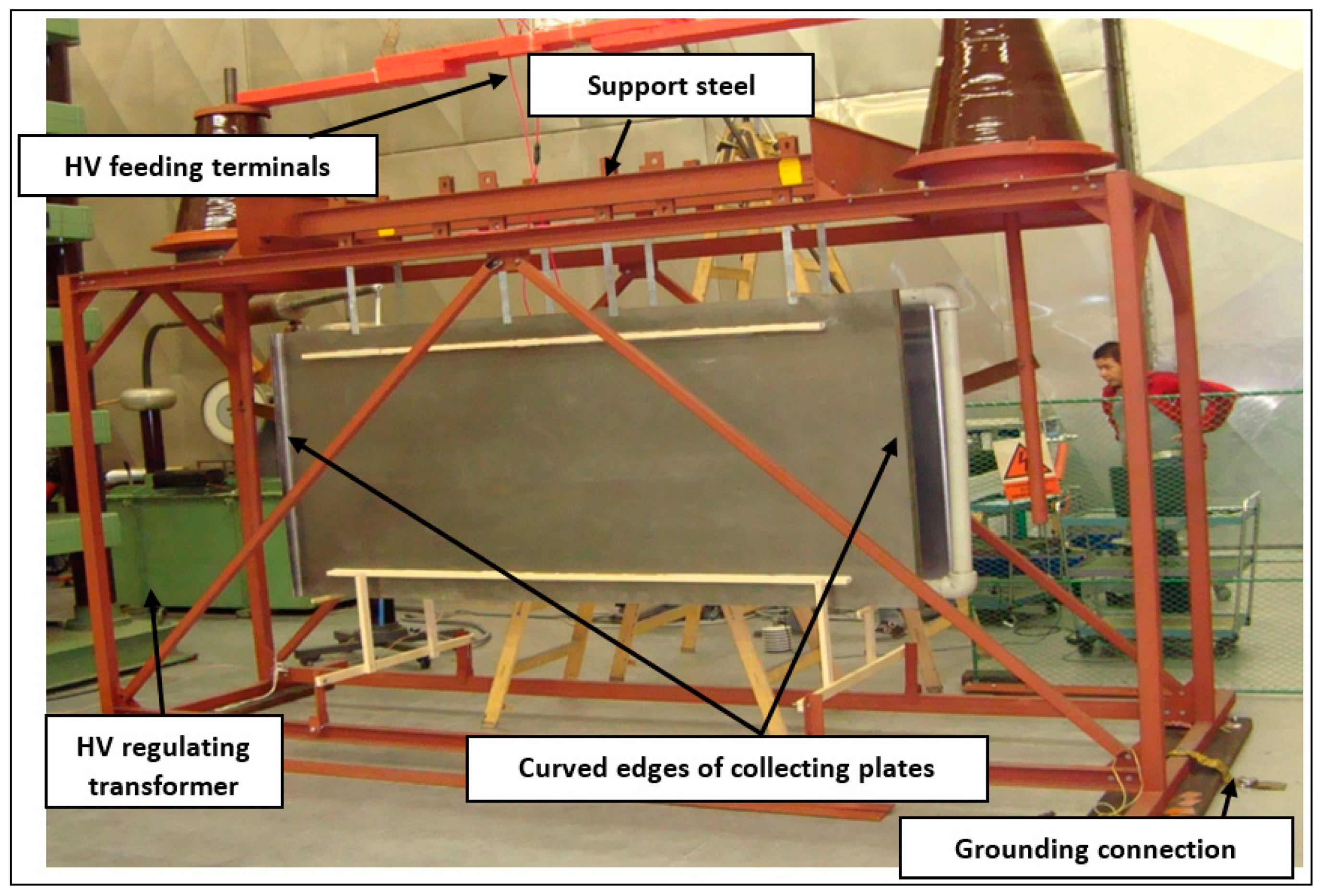
A 220V AC regulating transformer feeds the HV circuit through a switch to connect or disconnect the supply (Figure 11).

(2)

An HV transformer to step up the output voltage of the regulating transformer. The output voltage of the HV transformer was rectified through a rectifier circuit being immersed in the transformer oil with a smoothing capacitor bank consisting of two series capacitors; each one is 0.25 µF and 100 kV. The generated DC voltage was variable in the range 0–200 KV and was applied to the investigated WDESP through an 80 kΩ resistance for reducing the current in case a flash occurs in the WDESP (Figure 11).

(3)

The two collecting plates shaping the duct of the WDESP are made of steel and suspended vertically from a steel support with 125 × 250 cm dimensions of each plate with an adjusted 30 cm space between the two collecting plates. All the edges of the collecting plates were curved outside to avoid field concentration at the edges (Figure 1a and Figure 10).

(4)

The stressed discharge wires are steel, with the radii of 0.26, 0.935, and 1.975 mm, supported vertically between the plates, with two smooth spheres at each end of the discharge wires for avoiding field intensification, and the space between the wires is 14.5 cm (Figure 12b,c).

(5)

A pair of heaters are placed outside the collecting plates to increase the temperature of the ESP (Figure 1a,b).

To measure the corona-onset voltage and corona I–V characteristics of the single- and multi- (3, 5, and 7) discharge wires of WDESP, a micro-ammeter was connected between the collecting plates and the ground system (Figure 10 and Figure 11). When the micro-ammeter starts recording a reading over zero value, the corresponding value of the applied voltage is the corona-onset voltage of the WDESP. The corona current is increased by increasing the applied voltage of the precipitator. The corona-onset voltage and I–V characteristics of WDESP are measured by increasing the temperature of the incoming gases. The temperature ranges started from 300 to 1180 K. Different values of the wire radius (r_c = 0.26, 0.935, and 1.975 mm) were used for ESPs with 1, 3, 5, and 7 discharge wires, with the wire-to-wire (d) = 14.5 cm, and the spacing between the two plates (2H) being adjusted to 30. All the measurements were made in the HV laboratory, with pressure = 1001.3 kPa and a temperature = 22 °C. The maximum voltage applied to the set-up circuit without flash-over between the HV feeding terminals, and the steel supporting frame was about 120 kV. Therefore, the applied voltage increased safely up to 110 kV.

6. Results and Discussions

6.1. Accuracy of the Analytical Theoretical Calculation Methods

A comparison is made between the theoretical calculations using the CSM and FEM methods and the measured values in the laboratory.

Table 2. Accuracy of using charge simulation method (CSM) in calculating the corona-onset voltage of WDESP.

		rc = 0.26 mm		rc = 0.935 mm		rc = 1.975 mm
		Max. Error %		Max. Error %		Max. Error %
		Wire	Plate	Wire	Plate	Wire	Plate
Single-wire		0.035 × 10−6	7.53 × 10−3	1.79 × 10−6	1.04 × 10−3	2.88 × 10−6	6.12 × 10−3
Multi-discharge wires	3-wire	1.35 × 10−6	2.90 × 10−3	1.68 × 10−6	3.50 × 10−3	1.97 × 10−6	4.03 × 10−3
	5-wire	1.35 × 10−6	8.54 × 10−3	1.68 × 10−6	1.10 × 10−3	1.78 × 10−6	1.91 × 10−3
	7-wire	1.35 × 10−6	4.22 × 10−3	1.67 × 10−6	5.13 × 10−3	1.97 × 10−6	5.87 × 10−3

shows the accuracy of the calculation results of the electrostatic field of the WDESP and lists the maximum percentage error of the calculated potential of the stressed discharge wires and collecting plates, which are less than 10⁻⁶ and 10⁻³, respectively.

Based on Peek’s Formula for calculating the corona-onset voltage listed in ref. [20] (r_c = 5 mm, 2H = 30 mm, collecting plates with a diminution of 140 × 150 mm), a comparison has made between the results of CSM and this literature with the high-temperature incoming gases of WDESP. Figure 13 shows that the CSM results are more accurate than using Peek’s Formula to calculate the corona-onset voltage, especially with the high-temperature WDESP (over 900 K). This confirms the high accuracy of using CSM compared to using Peek’s Formula to calculate the corona-onset voltage of WDESP at high temperatures.

6.2. Electrostatic Field Calculations with High-Temperature WDESP

The distributions of the electrostatic field surrounding the central-discharge wire of the WDESP configuration (1, 3, 5, and 7 discharge wires; r_c = 0.26, 0.935, and 1.975 mm) with high-temperature incoming gases (300, 600, 900, and 1180 K) at the corona-onset voltage are shown in Figure 14, Figure 15, Figure 16 and Figure 17. The electrostatic field surrounding the central wire of all the WDESP configurations is higher at a lower temperature (300 K) and decreases with increasing temperatures (300 k through to 1180 K). This is because of the increase in the energy of ionic particles, so the corona-onset voltage occurs at lower voltage levels with an increasing WDESP temperature. Additionally, with the increase in the radius of the stressed wires, the electrostatic field surrounding the central wire of WDESP at the same temperature is decreased (Figure 14, Figure 15, Figure 16 and Figure 17). In case of increasing the number of discharge wires of WDESP (3, 5, 7 wire) at the same WDESP temperature and same wire radius, the electric field is decreased because the effect of shielding, which occurs on the central wires due to the other stressed discharge wires of WDESP (Figure 14, Figure 15, Figure 16 and Figure 17). Figure 18, Figure 19, Figure 20 and Figure 21 show the electric field in the Y-axis of WDESP, which starts from the discharge-wire surface to the collecting plate at high temperatures of 300, 600, 900, and 1180 K. The electric field close to the stressed wires and the collecting plates are higher at lower temperatures than the cases of high-temperature WDESP (Figure 18, Figure 19, Figure 20 and Figure 21).

Figure 14 shows the distribution of the electrostatic field around the stressed discharge wire for single-wire WDESP with the wire radius r_c of 0.26 and 1.975 mm and the corona onset voltage V_o of 14.939 and 30.868 kV, respectively. It is clear that with increasing the temperatures of the incoming gases from 300 to 1180 K, the electrostatic field around the discharge wires is decreased due to the increase in the ion mobility of the gases. Additionally, with the increase in the wire radius, the electrostatic field around the stressed wires is decreased, and this is in agreement with previous works.

Figure 15 shows the distribution of the electrostatic field around the central wire of the multi-discharge wires WDESP (three wire) with the radius r_c of 0.935 and 1.975 mm and the corona onset voltage V_o of 36.424 and 57.464 kV, respectively. Again, as in the previous case of single-wire WDESP, as the temperatures of the incoming gases increase, the electrostatic field around the discharge wires is decreased due to the increase in the ion mobility of the gases and the shield effect of the outer wires on the central wires; with the increase in the wire radius, the electrostatic field around the stressed wires is decreased, and this in agreement with previous works.

Figure 16 shows the distribution of the electrostatic field around the central wire of the multi-discharge wire WDESP (five-wire) with the radius r_c of 0.935 and 1.975 mm and the corona onset voltage V_o of 37.304 and 58.933 kV. Figure 17 shows the distribution of the electrostatic field around the central wire of the multi-discharge wire WDESP (seven-wire) with the radius r_c of 0.935 and 1.975 mm and the corona onset voltage V_o of 37.429 and 59.123 kV.

Figure 18 shows the electrostatic field along the Y-axis of the single-discharge wire WDESP at a high temperature with the wire radii r_c of 0.26, 0.935, and 1.975 mm. It is clear that the electrostatic field is high very close to surface of the stressed discharge wire and decreases gradually in the direction of the collecting plates, and this is agreement with the results of previous works. Additionally, with increasing temperatures, the overall electrostatic field in the WDESP unit is decreased due to an increase in the ion mobility of ion gases. With increasing the stressed discharge wire radius, the overall electrostatic field in the WDESP unit is decreased.

Figure 19, Figure 20 and Figure 21 show the electrostatic field along the Y-axis of the multi-discharge wire WDESP (three, five, and seven wires) at a high temperature with wire radii r_c of 0.26, 0.935, and 1.975 mm. The discussion is the same as in the case of the single-discharge wire.

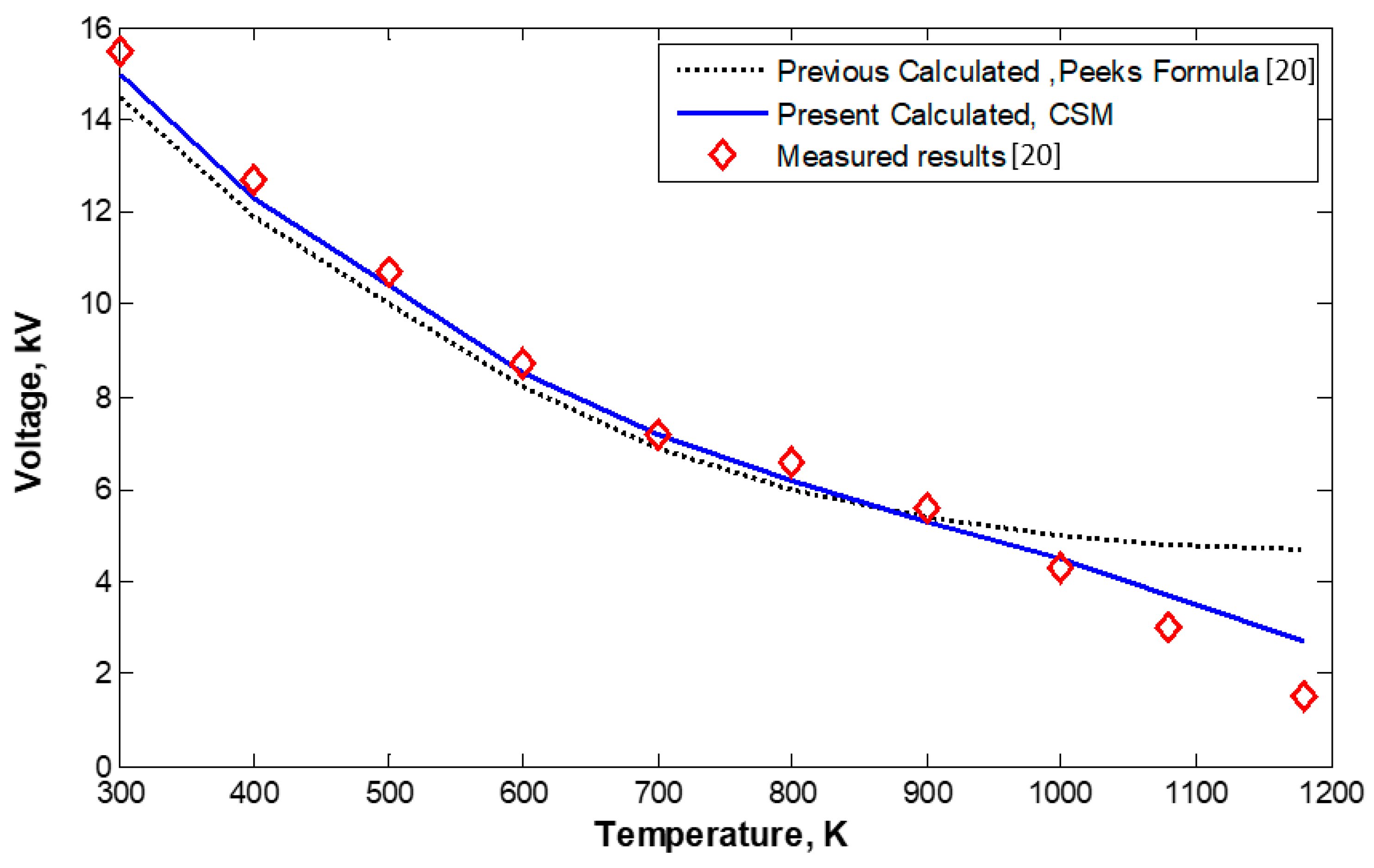
6.3. Effect of Temperature on Corona-Onset Voltage

Figure 22a shows a comparison between the calculated values of the corona-onset voltage based on CSM and the results of the experimental work of the WDESP single-discharge wire as influenced by the increasing temperature of the incoming gases and a varying wire radius of WDESP (0.26, 0.935, and 1.975 mm). The measured values agree with the calculated values using CSM. As the discharge-wire radius increases, the corona-onset voltage increases too. Additionally, the corona-onset voltage is decreased with an increase in the temperature of the incoming gases. This is due to the reduction in the electric field surrounding the stressed wires with the increase in the temperature of the incoming gases due to the increasing ion mobility of gases with increasing temperatures. Additionally, it is the same for multi-discharge WDESP configurations; the results of the corona-onset voltage are shown in Figure 22b–d, with the wire radii of 0.26, 0.935, and 1.975 mm. Again, the corona-onset voltage is decreased with the increase in the temperatures of incoming gases.

Effect of wire radius (r_c): At the same applied voltage and with a smaller discharge-wire radius, the corona-onset voltage gets smaller for the single-wire WDESP (Figure 22a), 3-wire WDESP (Figure 22b), 5-wire WDESP (Figure 22c), and 7-wire WDESP (Figure 22d). This is due to the corresponding electric field at the surface of the stressed wires.

Effect of the number of discharge wires: with an increase in the number of stressed discharge wires, a greater shielding effect will be found on the central wires of WDESP with an increase in the temperatures of incoming gases for 1, 3, 5, and 7 discharge wires at r_c = 0.26, 0.935, and 1.975 mm (Figure 22).

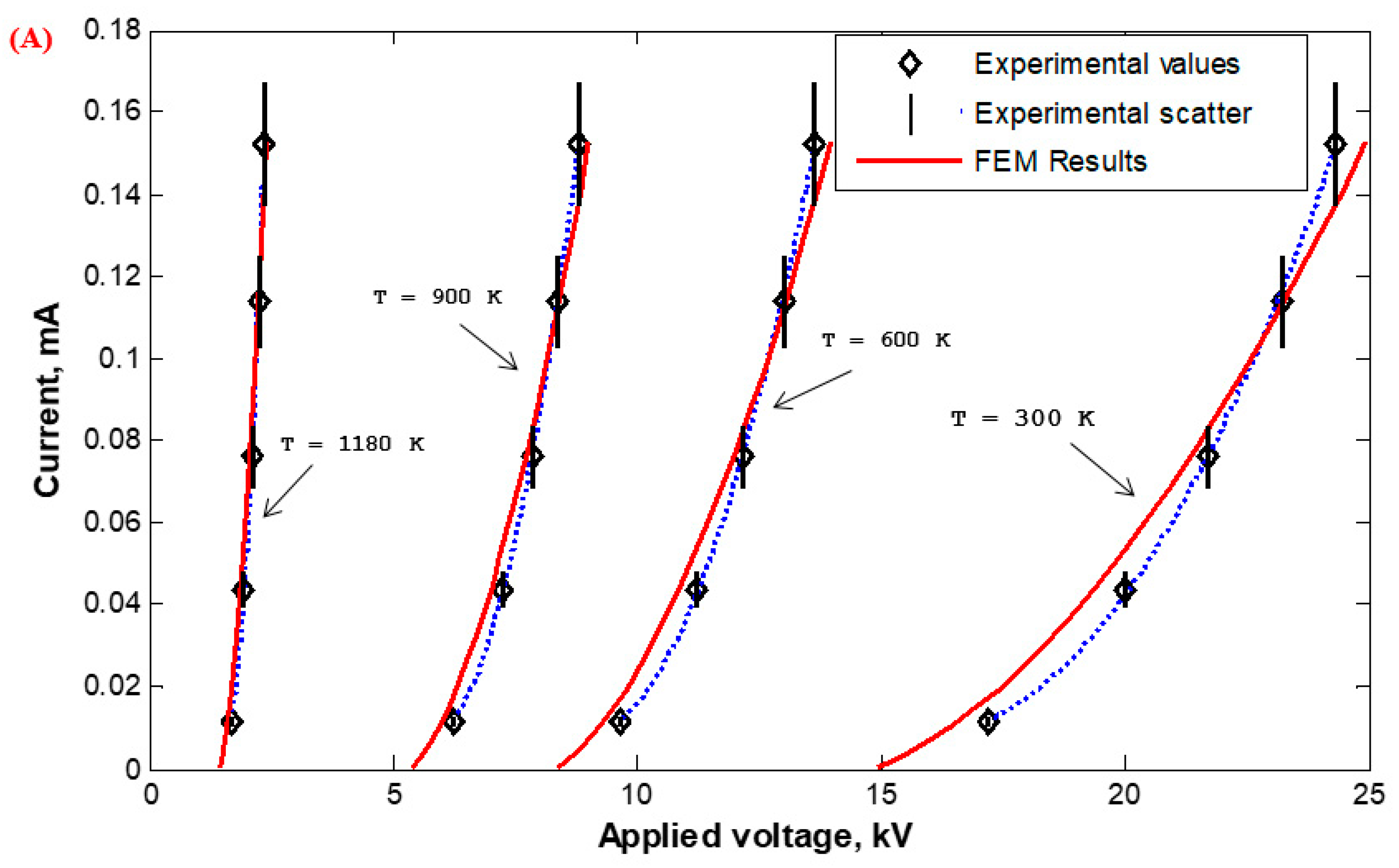
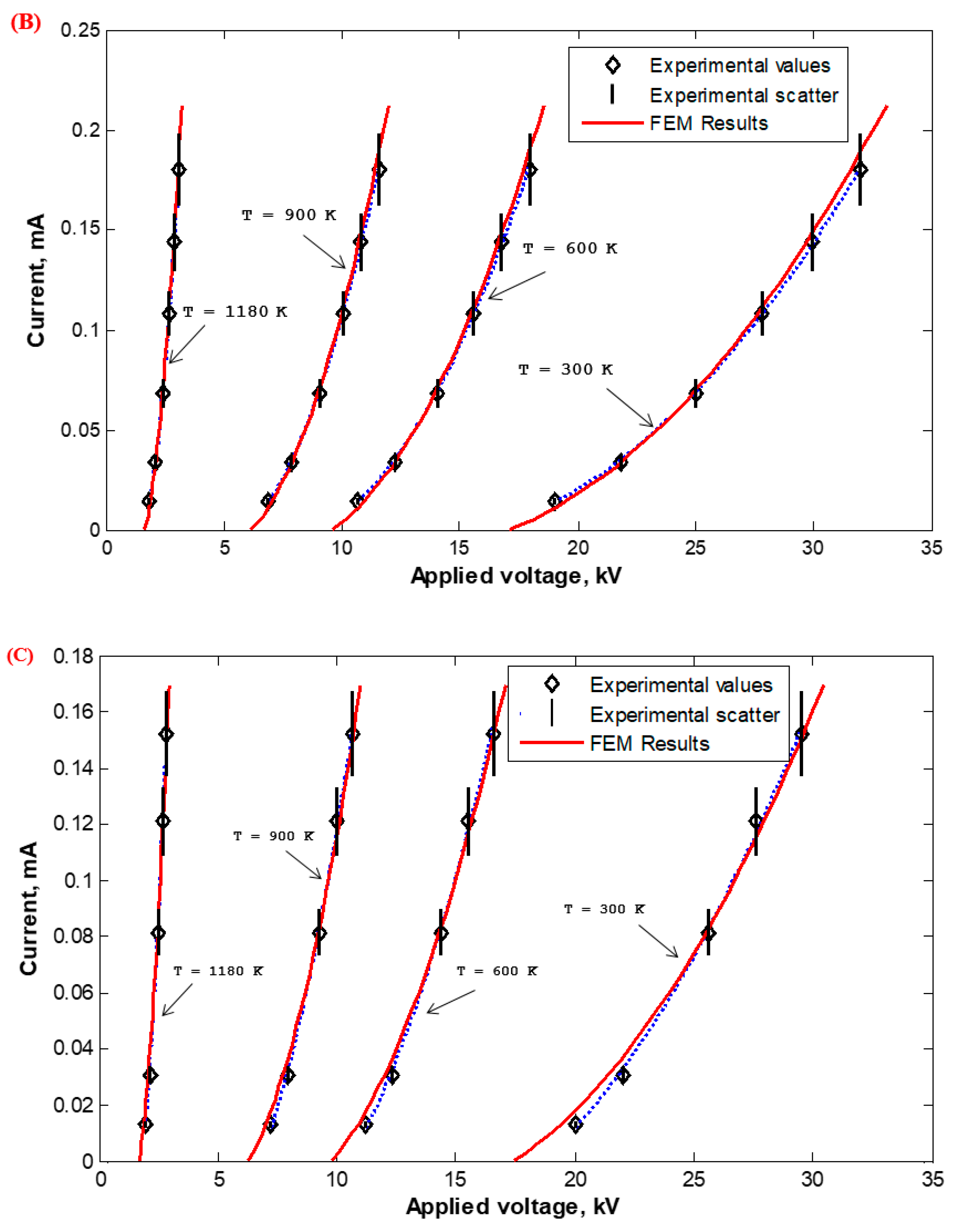
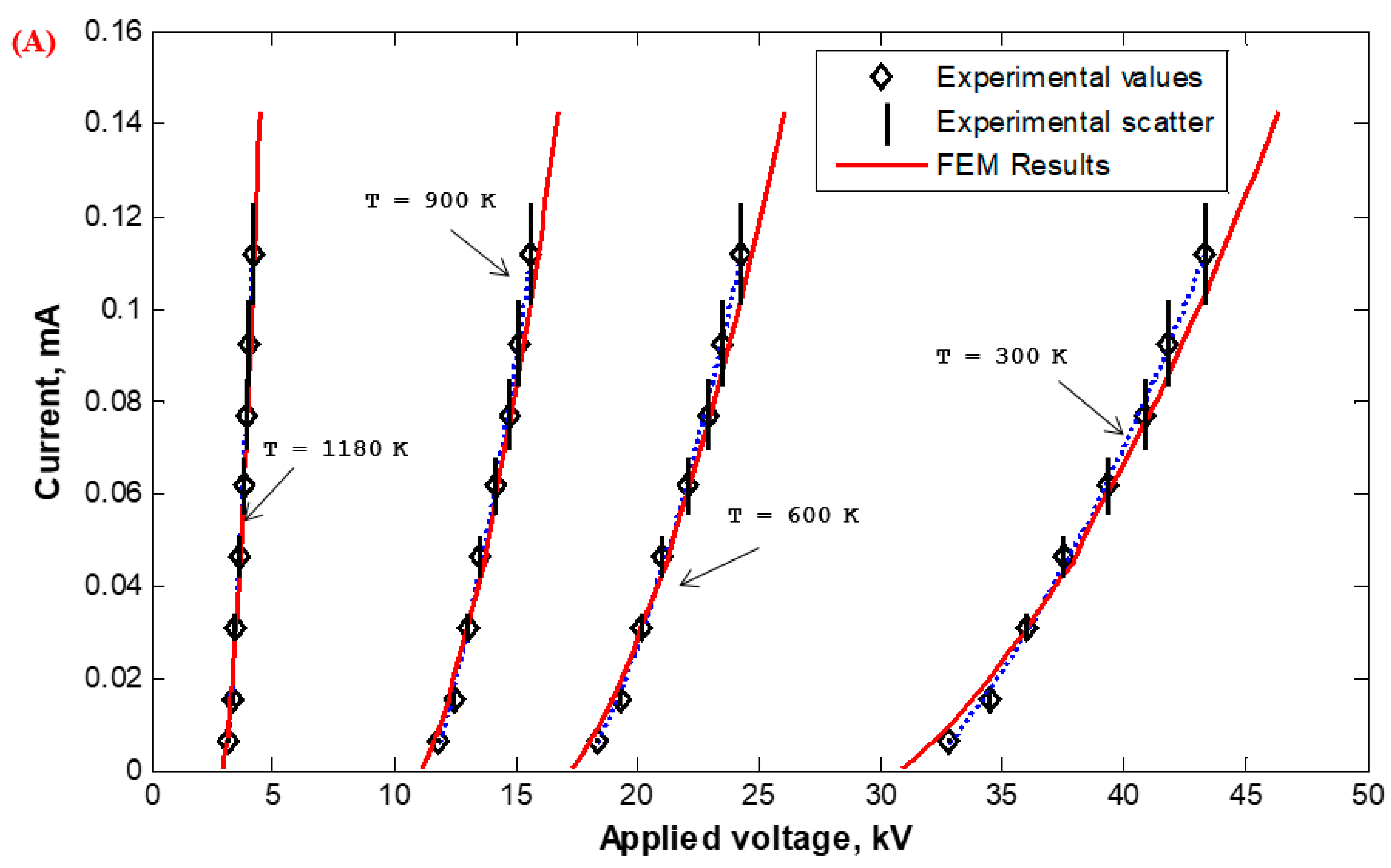
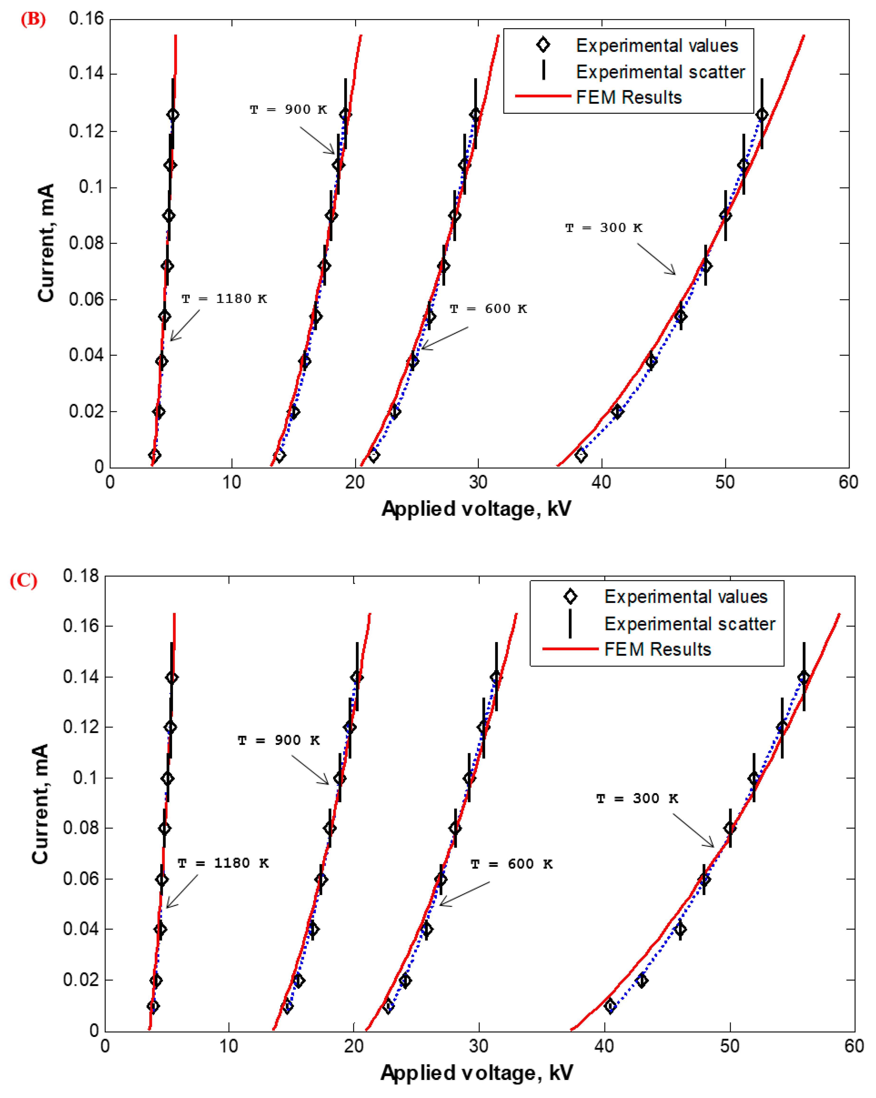
6.4. Effect of Temperature on I–V Characteristics Based on FEM and Measured Values Experimentally

Corona I–V properties were experimentally measured in the Laboratory of High Voltage Engineering of Czech Technical University (CTU) in Prague, Czech Republic, and calculated based on the FEM for wire-duct precipitators with different numbers of discharge wires (1, 3, 5, and 7) with varying wire radii (0.26 (Figure 23), 0935 (Figure 24), and 1.975 mm (Figure 25)) with high-temperature incoming gases from 300 to 1180 K. The wire-to-wire spacing was kept constant at 14.5 cm and the plate-to-plate spacing (2H) was also kept constant at 30 cm. It is satisfying that the characteristics calculated by FEM agreed reasonably—within the experimental scatter—with those measured experimentally, as shown in Figure 23, Figure 24 and Figure 25. The reduction in the corona-onset voltage with increasingly high temperatures (from 300 to 1180 K) is due to the corresponding field improvement at the wire surface due to an increase in the ionization coefficient at high temperatures. The corona current depends on how high the applied voltage is above the onset value. This is why the corona current at the same applied voltage increases with the increase in the incoming gas temperature.

Figure 23, Figure 24 and Figure 25 show the results of the FEM molding and measured values experimentally of the I–V characteristics of the WDESP with wire radii r_c of 0.26, 0.935, and 1.975 mm with high-temperature incoming gases of single-wire and multi-discharge wires (three, five, and seven wire). It is clear that the corona onset voltage is decreased with the increase in the temperatures of the incoming gases, and the discharge currents of the stressed wires I are increased rapidly with the increase in the temperatures of incoming gases at the same applied voltage. This is due to the increase in the ion mobility and space charge due to thermal diffusion.

Effect of wire radius (r_c): The smaller the wire radius, the smaller the onset voltage and the higher the corona current at the same applied voltage and plate-to-plate spacing for a single-discharge wire precipitator (Figure 23a, Figure 24a, and Figure 25a). Additionally, the smaller the wire radius is, the smaller the onset voltage and the higher the three-wire precipitator corona current at the same applied voltage and plate-to-plate spacing for the three-wire precipitator is (Figure 23b, Figure 24b, and Figure 25b), five-wire precipitators (Figure 23c, Figure 24c, and Figure 25c, and seven-wire precipitators (Figure 23d, Figure 24d, and Figure 25d). The reduction in the corona-onset voltage with the reduction in the wire radius is due to the corresponding field improvement at the wire surface. The corona current depends on how high the applied voltage is above the onset value. This is why the corona current at the same applied voltage increases with the decrease in the onset voltage. Irrespective of the value of the discharge wire radius (r_c), the characteristics calculated by FEM agree reasonably—within the experimental scatter—with those measured experimentally.

Effect of the number of discharge wires: The larger the number of discharge wires, the greater the shielding effect imposed on the central wires is, with a subsequent increase in the corona-onset voltage and decrease in the corona current emitted from the central wire at the same applied voltage and plate-to-plate spacing (Figure 23 for 1, 3, 5, and 7 at r_c = 0.26 mm; Figure 24 for 1, 3, 5, and 7 at r_c = 0.935 mm; and Figure 25 for 1, 3, 5, and 7 at r_c = 1.975 mm). It is quite obvious that the onset voltage and the corona I–V characteristics increase with a greater number of discharge wires as the shielding effect becomes more appreciable (Figure 23, Figure 24 and Figure 25). The reason for this is that the shielding effect on the central wires by the other discharge wires is followed by a reduction in the field at its surface and an increase in the onset voltage for the same applied voltage and same radius of the discharge wires (Figure 23, Figure 24 and Figure 25). Irrespective of the value of the number of discharge wires, the characteristics calculated by FEM agree reasonably—within the experimental scatter—with those measured experimentally.

7. Conclusions

An accurate numerical modeling/computation with the experimental verification of WDESP, taking into account the effect of high-temperature incoming gases, was discussed in this research work. The electrostatic field on the surface of the stressed wires (1, 3, 5, and 7 discharge wires) is higher at lower temperatures of WDESP, and it decreased with the increase in the temperatures of the incoming gases. Additionally, the electrostatic field along the Y-axis of WDESP is high near the stressed electrodes and decreased in the direction of the collecting plates. Additionally, with increasing temperatures, the electrostatic field decreased along the Y-axis of the WDESP. The modeling of the corona-onset voltage and corona I–V characteristics of the single- and multi- (3, 5, 7) discharge wire WDESP using CSM are agreed with those experimentally measured. Regarding the effect of the wire radius, the corona-onset voltage and corona I–V characteristics are increased with the increase in the radius of the stressed discharge wires of WDESP. Additionally, with an increase in the number of discharge wires, a greater shielding effect will occur on the central wires, a higher corona-onset voltage is obtained, and there is a decrease in the corona current at the same applied voltages. Finally, with the increasing temperatures of WDESP, the corona-onset voltage is decreased and the corona current is increased at the same applied voltage.

Regarding future work, the authors will start to study the effect of loading WDESP and repeat all the measurements in open air. Additionally, we will study the effect of high-speed incoming gases on WDESP in mathematical modeling and experimental results.

8. Limitations of the Work

The authors faced a lot of limitations, such as: (a) Building the experimental model in a high-voltage laboratory and the techniques of reading the results. (b) Difficulty in loading the WDESP with dust to measure its efficiency because all the measurements were performed in a high-voltage laboratory (clean room). If the WDESP is loaded, it should be outdoors and this is very hard due to safety regulations. (c) We could not increase the temperatures of the heaters over 1180 K.

References

1. Martínez Torres, J.; Pastor Pérez, J.; Sancho Val, J.; McNabola, A.; Martínez Comesaña, M.; Gallagher, J. A Functional Data Analysis Approach for the Detection of Air Pollution Episodes and Outliers: A Case Study in Dublin, Ireland. Mathematics 2020, 8, 225. [Google Scholar] [CrossRef] [Green Version]
2. Cacciola, M.; Pellicanò, D.; Megali, G.; Lay-Ekuakille, A.; Versaci, M.; Morabito, F.C. Aspects about air pollution prediction on urban environment. In Proceedings of the 4th IMEKO TC19 Symposium on Environmental Instrumentation and Measurements Protection Environment, Climate Changes and Pollution Control, Lecce, Italy, 3–4 June 2013; pp. 15–20, Code 102275. [Google Scholar]
3. Jin, X.-B.; Yang, N.-X.; Wang, X.-Y.; Bai, Y.-T.; Su, T.-L.; Kong, J.-L. Deep Hybrid Model Based on EMD with Classification by Frequency Characteristics for Long-Term Air Quality Prediction. Mathematics 2020, 8, 214. [Google Scholar] [CrossRef] [Green Version]
4. Lachatre, M.; Foret, G.; Laurent, B.; Siour, G.; Cuesta, J.; Dufour, G.; Meng, F.; Tang, W.; Zhang, Q.; Beekmann, M. Air Quality Degradation by Mineral Dust over Beijing, Chengdu and Shanghai Chinese Megacities. Atmosphere 2020, 11, 708. [Google Scholar] [CrossRef]
5. Qu, H.; Chan, W.; Xu, A.; Chung, K.; Lau, K.; Guo, P. Visual Analysis of the Air Pollution Problem in Hong Kong. IEEE Trans. Vis. Comput. Graph. 2007, 13, 1408–1415. [Google Scholar] [CrossRef] [Green Version]
6. Shimizu, K.; Sugiyama, T.; Samaratunge, M. Study of Air Pollution Control by Using Micro Plasma Filter. IEEE Trans. Ind. Appl. 2008, 44, 506–511. [Google Scholar] [CrossRef]
7. Abdel-Salam, M. Ionization and Deionization Processes in Gases, in High Voltage Engineering, Theory and Practice; Marcel Dekker: New York, NY, USA, 2000; pp. 81–112. ISBN1 0824704029. ISBN2 978-0824704025. [Google Scholar]
8. Zhang, L.; He, Y.; Liu, Y.; Yang, F.; He, T.; Liu, L.; Wang, S.; Liu, H. Temperature Analysis Based on Multi-Coupling Field and Ampacity Optimization Calculation of Shore Power Cable Considering Tide Effect. IEEE Access 2020, 8, 119785–119794. [Google Scholar] [CrossRef]
9. Salek, F.; Zamen, M.; Hosseini, S.V. Experimental study, energy assessment and improvement of hydroxy generator coupled with a gasoline engine. Energy Rep. 2020, 6, 146–156. [Google Scholar] [CrossRef]
10. Theodore, L. Air Pollution Control Equipment Calculations; John Wiley & Sons: New York, NY, USA, 2008; ISBN1 9780470209677. ISBN2 9780470255773. [Google Scholar] [CrossRef]
11. Moore, A.D. Electrostatics and Its Applications; John Wiley & Sons: New York, NY, USA, 1973; ISBN1 0471614505. ISBN2 978-0471614500. [Google Scholar]
12. Parker, K.; Warne, D.; Johns, A.T. Electrical Operation of Electrostatic Precipitators; Institution of Engineering and Technology (IET): London, UK, 2003; ISBN1 0852961375. ISBN2 9780852961377. [Google Scholar]
13. Zheng, C.; Zhang, X.; Yang, Z.; Liang, C.; Guo, Y.; Wang, Y.; Gao, X. Numerical simulation of corona discharge and particle transport behavior with the particle space charge effect. J. Aerosol Sci. 2018, 118, 22–33. [Google Scholar] [CrossRef]
14. Ziedan, H.A. Modeling of Corona Discharge in Wire-Duct Electrostatic Precipitators, Book; LAP LAMBERT Academic Publishing: Saarbrücken, Germany, 2016; ISBN 978-3847348160. [Google Scholar]
15. Wen, T.-Y.; Krichtafovitch, I.; Mamishev, A.V. Numerical study of electrostatic precipitators with novel particle-trapping mechanism. J. Aerosol Sci. 2016, 95, 95–103. [Google Scholar] [CrossRef]
16. Lu, Q.; Yang, Z.; Zheng, C.; Li, X.; Zhao, C.; Xu, X.; Cen, K. Numerical simulation on the fine particle charging and transport behaviors in a wire-plate electrostatic precipitator. Adv. Powder Technol. 2016, 27, 1905–1911. [Google Scholar] [CrossRef]
17. Farnoosh, N.; Adamiak, K.; Castle, G.S. Numerical calculations of submicron particle removal in a spike-plate electrostatic precipitator. IEEE Trans. Dielectr. Electr. Insul. 2011, 18, 1439–1452. [Google Scholar] [CrossRef]
18. Singer, H.; Steinbigler, H.; Weiss, P. A Charge Simulation Method for the Calculation of High Voltage Fields. IEEE Trans. Power Appar. Syst. 1974, PAS-93, 1660–1668. [Google Scholar] [CrossRef] [Green Version]
19. Ziedan, H.A.; Mizuno, A.; Sayed, A.; Ahmed, A. Onset voltage of corona discharge in wire-duct electrostatic precipitators. Int. J. Plasma Environ. Sci. Technol. 2010, 4, 36–44. [Google Scholar] [CrossRef]
20. Yan, P.; Zheng, C.; Xiao, G.; Xu, X.; Gao, X.; Luo, Z.; Cen, K. Characteristics of Negative DC Corona Discharge in a Wire–Plate Configuration at High Temperatures. Sep. Purif. Technol. 2014, 139, 5–13. [Google Scholar] [CrossRef]
21. Abdel-Salam, M.; Mazen, D. Transmission Line Electric Field Induction in Humans as Influenced by Corona Space Charge. Available online: http://cwl2004.powerwatch.org.uk/programme/posters/day3-abelsalem.pdf (accessed on 1 July 2020).
22. Medlin, A.J.; Morrow, R.; Fletcher, C.A.J. Calculation of monopolar corona at a high voltage DC transmission line with crosswinds. J. Electrost. 1998, 43, 61–77. [Google Scholar] [CrossRef]
23. Ziedan, H.A.; Tlustý, J.; Mizuno, A.; Sayed, A.; Ahmed, A. Corona current-voltage characteristics in wire-duct electrostatic precipitators, Theory versus Experiment. Int. J. Plasma Environ. Sci. Technol. 2010, 4, 154–162. [Google Scholar] [CrossRef]
24. Abdel-Salam, M.; Wiitanen, D. Calculation of corona onset voltage for duct-type precipitators. IEEE Trans. Ind. Appl. 1993, 29, 274–280. [Google Scholar] [CrossRef]
25. Bhatti, M.A. Fundamental Finite Element Analysis and Applications with Mathematica and MATLAB Computations; John Wiley & Sons: New York, NY, USA, 2005; ISBN 978-0-471-64808-6. [Google Scholar]
26. Deutsch, W. Úber die Dichtverteilung Unipolarer Lonenstrome. Ann. Physik 1933, 5, 589–613. [Google Scholar]
27. Sarma, M.P.; Janischewskyj, W. Analysis of Corona Losses on DC Transmission Lines: 1-Unipolar Lines. IEEE Trans. Power App. Syst. 1969, PAS-88, 718–731. [Google Scholar] [CrossRef]
28. Aboelsaad, M.M.; Shafai, L.; Rashwan, M. Numerical assessment of unipolar corona ionised field quantities using the finite-element method. IET Libr. 1989, 136, 79–86. [Google Scholar] [CrossRef]
29. Ziedan, H.A.; Tlustý, J.; Mizuno, A.; Sayed, A.; Ahmed, A.; Procházka, R. Finite element solution of corona I-V characteristics in ESP′s with multi discharge wires. Int. J. Plasma Environ. Sci. Technol. 2011, 5, 68–79. [Google Scholar] [CrossRef]
30. Abdel-Salam, M.; Al-Hamouz, Z. Finite Element Analysis of Monopolar Ionized Fields Including ion Diffusion. J. Phys. D Appl. Phys. 1993, 26, 2202–2211. [Google Scholar] [CrossRef]
31. Lisiak-Myszke, M.; Marciniak, D.; Bieliński, M.; Sobczak, H.; Garbacewicz, Ł.; Drogoszewska, B. Application of Finite Element Analysis in Oral and Maxillofacial Surgery—A Literature Review. Materials 2020, 13, 3063. [Google Scholar] [CrossRef] [PubMed]
32. Segerlind, L.J. Applied Finite Element Analysis; John Wiley & Sons: New York, NY, USA, 1984; ISBN 978-0-471-80662-2. [Google Scholar]
33. Jin, J.-M. The Finite Element Method of Electromagnetic, 3rd ed.; Wiley-IEEE Press: New York, NY, USA, 2014; ISBN 9781118571361. ASIN: 1118571363. [Google Scholar]
34. Hutton, D.V. Fundamentals of Finite Element Analysis; McGrow-Hill Companies, Inc.: New York, NY, USA, 2004. [Google Scholar]
35. Qiu, L.; Lv, Y.; Li, L. Finite Element Analysis for Stress and Magnetic Field of a 40 kA Protection Inductor. IEEE Trans. Appl. Supercond. 2010, 20, 1936–1939. [Google Scholar] [CrossRef]
36. Shimotani, T.; Sato, Y.; Sato, T.; Igarashi, H. Fast Finite-Element Analysis of Motors Using Block Model Order Reduction. IEEE Trans. Magn. 2016, 52, 7207004. [Google Scholar] [CrossRef] [Green Version]
37. Li, S.; Gallandat, N.A.; Mayor, J.R.; Habetler, T.G.; Harley, R.G. Calculating the Electromagnetic Field and Losses in the End Region of a Large Synchronous Generator Under Different Operating Conditions With 3-D Transient Finite-Element Analysis. IEEE Trans. Ind. Appl. 2018, 54, 3281–3293. [Google Scholar] [CrossRef]
38. Cacciola, M.; Morabito, F.C.; Polimeni, D.; Versaci, M. Fuzzy characterization of flawed metallic plates with eddy current tests. Prog. Electromagn. Res. 2007, 72, 241–252. [Google Scholar] [CrossRef] [Green Version]
Figure 1. Configuration of the wire-duct electrostatic precipitators (WDESP): (A) single-discharge wire and (B) multi-discharge wires.
Mathematics 08 01406 g001
Figure 2. Distribution of the simulated surface line charges and the set of boundary points in one quarter of the WDESP.
Mathematics 08 01406 g002
Figure 3. Flowchart for calculating the space-charge-free field in ESP.
Mathematics 08 01406 g003
Figure 4. Development of an avalanche.
Mathematics 08 01406 g004
Figure 5. Flowchart of the calculation of the corona-onset voltage of WDESP.
Mathematics 08 01406 g005
Figure 6. Electric-field flux lines extending from the stressed discharge wires to the collecting plates of WDESP.
Mathematics 08 01406 g006
Figure 7. Formation of the triangular elements.
Mathematics 08 01406 g007
Figure 8. Flowchart for calculating the corona I–V characteristics based on finite element method (FEM).
Mathematics 08 01406 g008
Figure 9. The volume around node (i, j) with the ith flux-tube.
Mathematics 08 01406 g009
Figure 10. An experimental model configuration of WDESP; Laboratory of High Voltage Engineering at Czech Technical University in Prague, Czech Republic.
Mathematics 08 01406 g010
Figure 11. Set-up of an experiment scheme diagram for measuring the corona of WDESP; Laboratory of High Voltage Engineering at Czech Technical University in Prague, Czech Republic.
Mathematics 08 01406 g011
Figure 12. Collecting plates’ configuration of WDESP at the Laboratory of High Voltage Engineering at Czech Technical University in Prague, Czech Republic: (A) collecting plates with a curved edge, (B) discharge wires, (C) top-ended sphere, and (D) bottom-ended sphere.
Mathematics 08 01406 g012
Figure 13. A comparison between the results of CSM and Peek’s Formula [20] in calculating the corona-onset voltage of single-wire WDESP with a high temperature.
Mathematics 08 01406 g013
Figure 14. The distribution of the electrostatic field around the stressed discharge wire for the single-wire WDESP: (A) rc = 0.26 mm, Vo = 14.939 kV; and (B) rc = 1.975 mm, Vo = 30.868 kV.
Mathematics 08 01406 g014aMathematics 08 01406 g014b
Figure 15. Distribution of the electrostatic field around the central wire of the multi-discharge wire WDESP (three-wire): (A) rc = 0.935 mm, Vo = 36.424 kV; and (B) rc = 1.975 mm, Vo = 57.464 kV.
Mathematics 08 01406 g015aMathematics 08 01406 g015b
Figure 16. Distribution of the electrostatic field around the central wire of the multi-discharge wire WDESP (five-wire): (A) rc = 0.935 mm, Vo = 37.304 kV; and (B) rc = 1.975 mm, Vo = 58.933 kV.
Mathematics 08 01406 g016aMathematics 08 01406 g016b
Figure 17. Distribution of the electrostatic field around the central wire of the multi-discharge wire WDESP (seven-wire): (A) rc = 0.935 mm, Vo = 37.429 kV; and (B) rc = 1.975 mm, Vo = 59.123 kV.
Mathematics 08 01406 g017aMathematics 08 01406 g017b
Figure 18. Electrostatic field along the Y-axis of the single-discharge wire WDESP at a high temperature: (A) rc = 0.26, (B) rc = 0.935, and (C) rc = 1.975 mm.
Mathematics 08 01406 g018aMathematics 08 01406 g018b
Figure 19. Electrostatic field along the Y-axis of the multi-discharge wire WDESP (three-wire) at a high temperature: (A) rc = 0. 26, (B) rc = 0. 935, and (C) rc = 1.975 mm.
Mathematics 08 01406 g019aMathematics 08 01406 g019b
Figure 20. Electrostatic field along the Y-axis of the multi-discharge wire WDESP (five-wire) at a high temperature: (A) rc = 0. 26, (B) rc = 0. 935, and (C) rc = 1.975 mm.
Mathematics 08 01406 g020aMathematics 08 01406 g020b
Figure 21. Electric field along the Y-axis of the multi-discharge wire WDESP (seven-wire) at a high temperature: (A) rc = 0. 26, (B) rc = 0. 935, and (C) rc = 1.975 mm.
Mathematics 08 01406 g021aMathematics 08 01406 g021b
Figure 22. The corona-onset voltage of WDESP with high-temperature incoming gases: (A) single-wire, (B) multi-discharge wire (three-wire), (C) multi-discharge wire (five-wire), and (D) multi-discharge wire (seven-wire).
Mathematics 08 01406 g022aMathematics 08 01406 g022bMathematics 08 01406 g022c
Figure 23. FEM molding and measured values experimentally for the I–V characteristics of WDESP (rc = 0.26 mm) with high-temperature incoming gases for (A) single wire, (B) multi-discharge wire (three-wire), (C) multi-discharge wire (five-wire), and (D) multi-discharge wire (seven-wire).
Mathematics 08 01406 g023aMathematics 08 01406 g023bMathematics 08 01406 g023c
Figure 24. FEM molding and measured values experimentally for the I–V characteristics of WDESP (rc = 0.935 mm) with high-temperature incoming gases for (A) single wire, (B) multi-discharge wire (three-wire), (C) multi-discharge wire (five-wire), and (D) multi-discharge wire (seven-wire).
Mathematics 08 01406 g024aMathematics 08 01406 g024bMathematics 08 01406 g024c
Figure 25. FEM molding and measured values experimentally for the I–V characteristics of WDESP (rc = 1.975 mm) with high-temperature incoming gases for (A) single wire, (B) multi-discharge wire (three-wire), (C) multi-discharge wire (five-wire), and (D) multi-discharge wire (seven-wire).
Mathematics 08 01406 g025aMathematics 08 01406 g025bMathematics 08 01406 g025c