Abstract
In this study, we introduce an efficient computational method to obtain an approximate solution of the time-dependent Emden-Fowler type equations. The method is based on the 2D-Bernstein polynomials (2D-BPs) and their operational matrices. In the cases of time-dependent Lane–Emden type problems and wave-type equations which are the special cases of the problem, the method converts the problem to a linear system of algebraic equations. If the problem has a nonlinear part, the final system is nonlinear. We analyzed the error and give a theorem for the convergence. To estimate the error for the numerical solutions and then obtain more accurate approximate solutions, we give the residual correction procedure for the method. To show the effectiveness of the method, we apply the method to some test examples. The method gives more accurate results whenever increasing for linear problems. For the nonlinear problems, the method also works well. For linear and nonlinear cases, the residual correction procedure estimates the error and yields the corrected approximations that give good approximation results. We compare the results with the results of the methods, the homotopy analysis method, homotopy perturbation method, Adomian decomposition method, and variational iteration method, on the nodes. Numerical results reveal that the method using 2D-BPs is more effective and simple for obtaining approximate solutions of the time-dependent Emden-Fowler type equations and the method presents a good accuracy.
1. Introduction
The heat equation which expresses the diffusion of heat can be given by the following form [1,2,3]:
subject to
where represents the temperature and t the time, and a is an integer, is a constant and the term is the nonlinear heat source, where and h are some smooth functions. For the steady case with and , Equation (1) is the Emden-Fowler equation [4,5,6], that is,
In this work, we study the numerical solution, which is a simply applied and effective method, of the time-dependent Emden-Fowler type equations. First, the heat-type Equation (1) is considered. To solve Equation (1) by the proposed numerical technique, an operational matrix based on two-dimensional Bernstein polynomials is constructed. Second, with the same notations, we obtain the approximate solutions of the following wave-type equation:
subject to
The main issue arisen in the analysis of Equations (1) and (4) is treating the singularity at To overcome this singularity behavior at this point, there are some semi-analytical methods which are used to solve nonlinear problems in the literature such as Adomian’s decomposition method (ADM) [1,5], homotopy analysis method (HAM) [9,10,11,12], variational iteration method (VIM) [4,13,14,15,16,17], and homotopy perturbation method (HPM) [18,19,20,21,22]. Wazwaz [5] used ADM to get approximate analytic solutions of (3). He obtained more accurate results for several examples. Another study by Wazwaz [1] for time-dependent Emden-Fowler equation was given with a generalization of the previous work. He employed ADM to solve Equations (1) and (4) and obtained convergent results for several examples. Chowdhury and Hashim [3] applied HPM to get approximate analytical solutions of (1) and (4). Bataineh et al. [6] applied HAM to solve the problems (1) and (4). Belal et al. [23] used VIM to solve this problem.
Since the operational matrices method can achieve the singularity behavior at the point , it has been applied to some singular problems. Yousefi and Behroozifar [24] applied the Bernstein operational matrix to solve the Emden-Fowler equation for the steady-state case. The same problem was considered by Gupta and Sharma [25] and solved by the Taylor series method. Another work to solve the steady-state problem was given by Wazwaz et al. [26]. They applied VIM to the problem. When only the Lane–Emden equation is considered, there are many numerical methods that depend on ADM [27,28], VIM [29,30,31,32], HPM [8,33], and operational matrices method [34] or Bernstein collocation method [35] were used to get analytic or numerical solutions.
The methods based on operational matrix of differentiation were given in various forms in the literature. Some of them were constituted by Chebyshev polynomials [36], Legendre polynomials [37], and Bernstein polynomials [38,39,40,41,42,43,44]. One of the common properties of these polynomials is the basis of polynomial spaces. On the other hand, because of Bernstein polynomials are dense in [45] and thus yields good approximation results, they have been used often recently to solve the problems in two-dimensions. The Bernstein operational matrices method is also known as the Bernstein matrix method [44] and Bernstein series solution [35].
In this work, we shall develop a method based Bernstein operational matrices to solve the nonlinear problem 1. The method is applied easily and presents a good accuracy. We first give Bernstein polynomials in 1D and 2D in Section 2. The matrix representations of the approximate functions and their operational matrices for both dimensions are given next. Section 3 presents the method of solution for heat-type and wave-type equations. In Section 4, we constitute the residual correction procedure both to estimate the absolute error and to get the corrected approximate solutions. The most important property of the procedure can be applied even if the exact solution is unknown. Section 5 contains some examples including linear and nonlinear models to demonstrate the applicability of the method. First, we apply the method to time-dependent Lane–Emden type problems and singular wave-type equations. We perform the method for different number of nodes. The numerical results show that increasing number of nodes gives a sequence of approximations, which converges to the exact solution, for linear problems. The method also gives good results for nonlinear problems. Residual correction procedure estimates the error in general. On the other hand, the corrected approximate solutions can be obtained and its error is less than the approximate solution. We compare the approximate solutions obtained by the method with the approximate solutions obtained by ADM, HPM, HAM, and VIM by calculating the error on some nodes in . In the last section, we summarize the results.
2. 2D Bernstein Polynomials (2D-BPs) and Their Operational Matrices
In this section, because of defining two-dimensional Bernstein polynomials easily, we will give one-dimensional, Bernstein polynomials first. The Bernstein polynomials of degree m (1D-BPs) on are defined as [46]
where with if or . Equation (6) can be rewritten as
Let be any real-valued continuous function. The truncated Bernstein polynomials approximation of y is
where
To ease computational complexity, the matrix representations of
are to be determined. Let and be and matrices respectively for as follows:
Then, the polynomial is given by
which gives the identity:
where
Note that
and
where
The Bernstein polynomials of degree (2D-BPs) on are defined as [47,48]
which can be rewritten as [45]
Theorem 1
([45]). Let . The set of all two-dimensional Bernstein polynomials on the box Ω is dense in .
Figure 1 shows the two components of the two-dimensional Bernstein polynomials of order (5,5).
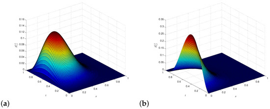
Figure 1.
Two components of the two-dimensional Bernstein polynomials of order (5,5): (a) and (b) .
Now, assume that y is a real-valued function defined on We want to approximate by the truncated 2D-BPs series, i.e.,
The partial derivatives and can be approximated as
Hence, we get
For the higher-order derivatives, we have
3. Solving Heat-Type and Wave-Type Equations by 2D-BPs
To approximate the solution of (1) subject to the initial condition (2), one substitutes the identities in (25), (26), and (27) into (1). The residual are given by
The conditions (2) then yield
Thus, we have equations. By solving these equations by the command ’fsolve’ which uses Newton’s method for the unknown coefficients , we can find the matrix so that is obtained.
In this study, we select the collocation nodes as Newton–Cotes points
When applied to the wave-type Equation (4), we get the following:
4. Error Analysis
In this section, we first give the Bernstein series that converges for the function in . The residual correction procedure is given to estimate the absolute error and to obtain corrected approximate solutions. To determine the convergence of the method, we define the constant as follows.
Definition 1.
Suppose that and for , then
where all partial derivatives of f of order are bounded in magnitude , which is
Now, the main theorem of function approximation using 2D-BPs are stated as follows.
Theorem 2.
Consider and . Let . Next, suppose that
Approximating by in the space as
where is the best approximation out of and supposing that
then
Proof.
Let
Therefore, by considering Definition 1 and by taking , we get
By considering Taylor’s expansion formula in Definition 1, one has
Hence, we get
This concludes the proof. ☐
Now, we constitute residual correction procedure for the problem. Let be the exact and the 2D-BPs approximate solutions of Equation (1), respectively. Writing as the error, then
where
Substituting the approximate solution along with the constructed operational matrix in (42) yields the residual equation for the error as
To solve Equation (43) numerically, we compute it at the following collocation points:
Applying the proposed method to (43) with the given initial conditions gives us the coefficient matrix so that we get an approximate solution for the error. Hence, is another approximate solution, which is called the corrected 2D-BPs approximate solution for the problem. In practice, selecting yields better approximation results.
The solution improves the approximation provided that
Similar definitions and results can be given for the wave-type Equation (4).
5. Application to Several Test Problems
The applicability of the proposed 2D-BPS method is demonstrated via several test problems. To simulate the results, three types of equations are selected. Our results are compared with the methods of ADM, HPM, VIM, and HAM with . We use the Newton–Cotes points (32) and Maple 15 to simulate the numerical outlets with 50-digit precision.
5.1. Time-Dependent Lane–Emden Type Problems
Example 1.
Consider
subject to
The exact solution is [1,2,3,4]:
We perform the method to the problem for various , and . The results are given in Table 1 and Table 2. As seen from the tables, increasing n gives the decreasing error sequence while the computational time increases. On the other hand, residual correction procedure estimates the error well for . The corrected solutions are more accurate than the solutions for . We give the computational costs of the method in Table 3. Increasing yields more computational costs which means that the method needs more computational times, numbers of multiplications, summations, assignments, and storages for big . As a result, we can say that the numbers are selected as not too big or not too small. It seems to be suitable for selecting around 10 for Example 1.

Table 1.
The norms of absolute errors, the estimation of the errors by using the residual correction procedure, and the errors obtained by the corrected approximate solutions of Example 1 for .
Table 2.
The results for Example 1 and .
Table 3.
The computational costs of the obtaining of the method for in the Maple code for Example 1.
The graphs of , and are plotted in Figure 2 which also depicts the absolute errors of the 5th-order approximate solutions of ADM, HPM, HAM and VIM [1,2,3,4]. We also give a comparison for the method with HAM and VIM in Table 4 for different nodes number. It can be seen from Figure 2 and Table 4 that the corrected 2D-BPs approximate solution yields better approximate results than the results obtained by ADM, HPM, HAM, and VIM. Moreover, the residual correction procedure estimates the error more accurately.
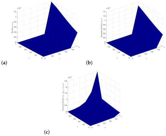
Figure 2.
(a) absolute error, (b) estimated absolute error, and (c) corrected absolute error for 2D-BPs solution for Example 1.
Table 4.
The results of the 2D-BPM, HAM, and VIM for Example 1.
5.2. Singular Wave-Type Equations
Example 2.
We consider now
where the exact solution is
The solution in series form by ADM [1], HAM [2], and HPM [3] is
We applied the method to the problem for various . We can say from Table 5 that the norm of the absolute error decreases when increases. The procedure estimates the error well and the corrected solutions are better than the solutions in the norm. The absolute error and corrected absolute error for are shown in Figure 3. We also give the solutions of the problem by ADM, HPM, and HAM [1,2,3] to make a comparison in the same figure. We can conclude from this figure that the corrected absolute error is better than the absolute error, also better than the absolute error of ADM, HPM, and HAM.
Table 5.
The norms of absolute errors, the estimation of the errors by using the residual correction procedure, and the errors obtained by the corrected approximate solutions of Example 2 for and .
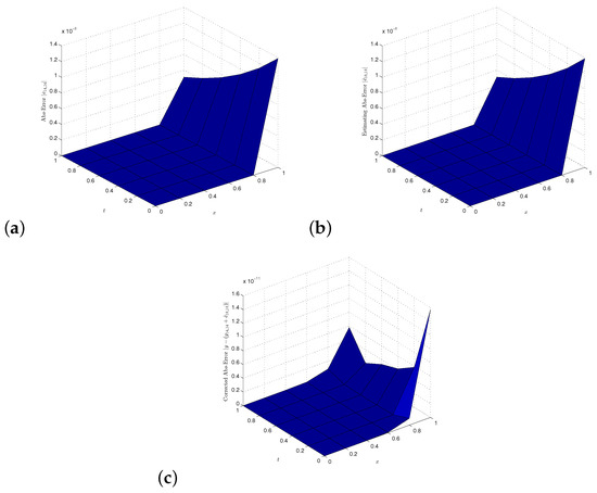
Figure 3.
(a) absolute error; (b) estimated absolute error; (c) corrected absolute error for 2D-BPs solution for Example 2.
5.3. Nonlinear Models
Example 3.
Consider
The exact solution of the problem [1,2,3,4] is We apply the method to the linear problem for various and apply the procedure for The results are given in Table 6 and Table 7. As seen from the tables, increasing yields more accurate results, whereas the computational times increase. On the other hand, the proposed method yields a much better approximate solution than the solutions obtained by ADM, HAM, and HPM [1,2,3], of order 5. We plot the error, the estimation of the error, and the corrected error for and in Figure 4. We can say from the figures that the estimation by using the procedure fits the error well and the corrected error is smaller than the error.
Table 6.
The norms of absolute errors, the estimation of the errors by using the residual correction procedure, and the errors obtained by the corrected approximate solutions of Example 3 for .
Table 7.
The results of the 2D-BPM and HAM for Example 3.
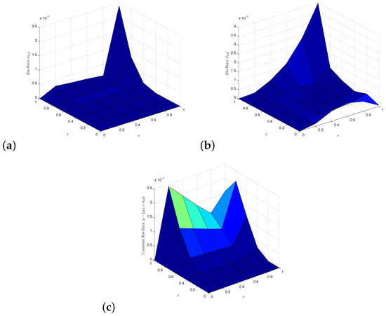
Figure 4.
(a) absolute error; (b) estimated absolute error; (c) corrected absolute error for 2D-BPs solution for Example 3.
6. Conclusions
In this study, we have proposed a numerical method to solve time-dependent Emden-Fowler type equations. In the numerical scheme, the 2D-BPs are utilized. The residual correction procedure is applied to estimate the error of the approximate solution. By using the suggested procedure, we obtain a new approximate solution which is more accurate than the 2D-BPs approximate solution. The error analysis as well as convergence of the proposed method have been investigated. We applied the method to several test problems including linear and nonlinear problems and also compared with some other methods to show the efficiency of the new method. As seen from the results of text examples, increasing the node numbers yields a sequence which converges to the exact solution for all examples in the norm. The computational times and necessary operations in the code increase if increases. Hence, the optimum values are observed around 10. The procedure estimates the error with a good accuracy for . In addition, by using the procedure, more accurate results are obtained. We can conclude that the obtained results are consistent with the results of ADM, HPM, HAM, and VIM. Especially for the nonlinear problem, the method gives better approximate solutions with respect to the semi-analytic methods.
Author Contributions
Conceptualization, A.S.B., O.R.I., A.-K.A., M.S. and I.H.; methodology, A.S.B., O.R.I., A.-K.A. and M.S.; software, A.S.B., O.R.I., A.-K.A. and M.S.; validation, A.S.B., O.R.I., A.-K.A., M.S. and I.H.; formal analysis, A.S.B., O.R.I., A.-K.A. and M.S.; investigation, A.S.B., O.R.I., A.-K.A. and M.S.; writing-original draft preparation, A.S.B., O.R.I., A.-K.A. and M.S.; writing-review and editing, A.S.B., O.R.I., A.-K.A., M.S. and I.H.; funding acquisition, I.H.. All authors have read and agreed to the published version of the manuscript.
Funding
We are grateful for the financial support received from the Universiti Kebangsaan Malaysia under the research grant GP-2019-K006388.
Conflicts of Interest
All authors declare that they have no conflict of interest.
References
- Wazwaz, A.M. Analytical solution for the time-dependent Emden-Fowler type of equations by Adomian decomposition method. Appl. Math. Comput. 2005, 166, 638–651. [Google Scholar] [CrossRef]
- Bataineh, A.S.; Noorani, M.S.M.; Hashim, I. Solutions of time-dependent Emden-Fowler type equations by homotopy analysis method. Phys. Letts. A 2007, 371, 72–82. [Google Scholar] [CrossRef]
- Chowdhury, M.S.H.; Hashim, I. Solutions of time-dependent Emden-Fowler type equations by homotopy-perturbation method. Phys. Letts. A 2007, 368, 305–313. [Google Scholar] [CrossRef]
- Batiha, K. Approximate analytical solutions for time-dependent Emden-Fowler-type equations by variational iteration method. Am. J. Appl. Sci. 2007, 4, 439–443. [Google Scholar] [CrossRef]
- Wazwaz, A.M. Adomian decomposition method for a reliable treatment of the Emden-Fowler equation. Appl. Math. Comput. 2005, 161, 543–560. [Google Scholar] [CrossRef]
- Bataineh, A.S.; Noorani, M.S.M.; Hashim, I. Homotopy analysis method for singular IVPs of Emden-Fowler type. Commun. Nonlinear Sci. Numer. Simulat. 2009, 14, 1121–1131. [Google Scholar] [CrossRef]
- Chandrasekhar, S. An Introduction to the Study of Stellar Structure; Dover Publications: New York, NY, USA, 1957. [Google Scholar]
- Ramos, J.I. Series approach to the Lane–Emden equation and comparison with the homotopy perturbation method. Chaos Solitons Fractals 2008, 38, 400–408. [Google Scholar] [CrossRef]
- Liao, S.J. The Proposed Homotopy Analysis Technique for the Solution of Nonlinear Problems. Ph.D. Thesis, Shanghai Jiao Tong University, Shanghai, China, 1992. [Google Scholar]
- Liao, S.J. Beyond Perturbation: Introduction to Homotopy Analysis Method; Chapman and Hall/CRC Press: Boca Raton, FL, USA, 2003; p. 321. [Google Scholar]
- Liao, S.J. On the homotopy analysis method for nonlinear problems. Appl. Math. Comput. 2004, 147, 499–513. [Google Scholar] [CrossRef]
- Liao, S.J. Comparison between the homotopy analysis method and homotopy perturbation method. Appl. Math. Comput. 2005, 169, 1186–1194. [Google Scholar] [CrossRef]
- He, J.H. A new approach to nonlinear partial differential equation. Commun. Nonlinear Sci. Numer. Simul. 1997, 2, 230–235. [Google Scholar] [CrossRef]
- He, J.H. Approximate analytical solution for seepage flow with functional derivatives in porous media. Comput. Methods Appl. Mech. Eng. 1998, 167, 57–68. [Google Scholar] [CrossRef]
- He, J.H. Approximate solution of nonlinear differential equations with convolution roduct nonlinearities. Comput. Methods Appl. Mech. Eng. 1998, 167, 69–73. [Google Scholar] [CrossRef]
- He, J.H. Variational iteration method-a kind of nonlinear analytical technique: Some examples. Int. J. Non-Linear Mech. 1999, 34, 699–708. [Google Scholar] [CrossRef]
- He, J.H. Variational iteration method for autonomous ordinary differential systems. Appl. Math. Comput. 2000, 114, 115–123. [Google Scholar] [CrossRef]
- He, J.H. Homotopy perturbation method: A new nonlinear analytical technique. Appl. Math. Comput. 2003, 135, 73–79. [Google Scholar] [CrossRef]
- He, J.H. Asymptotology by homotopy perturbation method. Appl. Math. Comput. 2004, 156, 591–596. [Google Scholar] [CrossRef]
- He, J.H. The homotopy perturbation method for nonlinear oscillators with discontinuities. Appl. Math. Comput. 2004, 151, 287–292. [Google Scholar] [CrossRef]
- He, J.H. Application of homotopy perturbation method to nonlinear wave equations. Chaos Solitons Fractals 2005, 26, 695–700. [Google Scholar] [CrossRef]
- He, J.H. Homotopy perturbation method for bifurcation of nonlinear problems. Int. J. Nonlinear Sci. Numer. Simul. 2005, 6, 207–208. [Google Scholar] [CrossRef]
- Batiha, B.; Noorani, M.S.N.; Hashim, I. Application of variational iteration method to heat and wave-like equations. Phys. Letts. A 2007, 369, 55–61. [Google Scholar] [CrossRef]
- Yousefi, S.A.; Behroozifar, M. Operational matrices of Bernstein polynomials and their applications. Int. J. Syst. Sci. 2010, 41, 709–716. [Google Scholar] [CrossRef]
- Gupta, V.G.; Sharma, P. Solving singular initial value problems of Emden-Fowler and Lane–Emden type. Int. J. Appl. Math. Comput. Sci. 2009, 1, 206–212. [Google Scholar]
- Wazwaz, A.M. Solving two Emden-Fowler type equations of third order by the variational iteration method. Appl. Math. Inf. Sci. 2015, 9, 2429–2436. [Google Scholar]
- Wazwaz, A.-M. A new algorithm for solving differential equations of Lane–Emden type. Appl. Math. Comput. 2001, 118, 287–310. [Google Scholar] [CrossRef]
- Rach, R.; Wazwaz, A.M.; Duan, J.S. The Volterra integral form of the Lane–Emden equation: New derivations and solution by the Adomian decomposition method. J. Appl. Math. Comput. 2015, 47, 365–379. [Google Scholar] [CrossRef]
- Dehghan, M.; Shakeri, F. Approximate solution of a differential equation arising in astrophysics using the variational iteration method. New Astron. 2008, 13, 53–59. [Google Scholar] [CrossRef]
- Yildirim, A.; Ozis, T. Solutions of singular IVPs of Lane–Emden type by the variational iteration method, Nonlinear Analy. Theory Methods Appl. 2009, 70, 2480–2484. [Google Scholar] [CrossRef]
- Zomot, N.H.; Ababneh, O.Y. Solution of differential equations of Lane–Emden type by combining integral transform and variational iteration method. Nonlinear Analy. Diff. Equ. 2016, 4, 143–150. [Google Scholar] [CrossRef]
- Ghorbani, A.; Bakherad, M. A variational iteration method for solving nonlinear Lane–Emden problems. New Astron. 2017, 54, 1–6. [Google Scholar] [CrossRef]
- Rafig, A.; Hussain, S.; Ahmed, M. General homotopy method for Lane–Emden type differential equations. Int. J. Appl. Math. Mech. 2009, 5, 75–83. [Google Scholar]
- Kumar, N.; Pandey, R. Solution of the Lane–Emden equation using the Bernstein operational matrix of integration. ISRN Astron. Astrophys. 2011, 2011, 351747. [Google Scholar] [CrossRef]
- Isik, O.R.; Sezer, M. Bernstein series solution of a class of Lane–Emden type equations. Math. Probl. Eng. 2013, 2013, 423797. [Google Scholar] [CrossRef]
- Bhrawya, A.H.; Alofi, A.S. The operational matrix of fractional integration for shifted Chebyshev polynomials. Appl. Math. Lett. 2013, 26, 25–31. [Google Scholar] [CrossRef]
- Kashkari, B.S.; Syam, M.I. Fractional-order Legendre operational matrix of fractional integration for solving the Riccati equation with fractional order. Appl. Mathe. Comput. 2016, 290, 281–291. [Google Scholar] [CrossRef]
- Pandey, R.K.; Kumar, N. Solution of Lane–Emden type equations using Bernstein operational matrix of differentiation. New Astron. 2012, 17, 303–308. [Google Scholar] [CrossRef]
- Maleknejad, K.; Basirat, B.; Hashemizadeh, E. A Bernstein operational matrix approach for solving a system of high order linear Volterra-Fredholm integro-differential equations. Math. Comput. Model. 2012, 55, 1363–1372. [Google Scholar] [CrossRef]
- Yousefi, S.A.; Behroozifar, M.; Dehghan, M. The operational matrices of Bernstein polynomials for solving the parabolic equation subject to specification of the mass. J. Comput. Appl. Math. 2011, 335, 5272–5283. [Google Scholar] [CrossRef]
- Yousefi, S.; Behroozifar, M.; Dehghan, M. Numerical solution of the nonlinear age-structured population models by using the operational matrices of Bernstein polynomials. Appl. Math. Model. 2012, 36, 945–963. [Google Scholar] [CrossRef]
- Maleknejad, K.; Hashemizadeh, E.; Basirat, B. Computational method based on Bernstein operational matrices for nonlinear Volterra-Fredholm-Hammerstein integral equations. Commun. Nonlinear Sci. Numer. Simulat. 2012, 17, 52–61. [Google Scholar] [CrossRef]
- Parand, K.; Hossayni, S.A.; Rad, J.A. Operation matrix method based on Bernstein polynomials for the Riccati differential equation and Volterra population model. Appl. Math. Model. 2016, 40, 993–1011. [Google Scholar] [CrossRef]
- Bataineh, A.S.; Isik, O.R.; Hashim, I. Bernstein method for the MHD flow and heat transfer of a second grade fluid in a channel with porous wall. Alex. Eng. J. 2016, 55, 2149–2156. [Google Scholar] [CrossRef]
- Nemati, A. Numerical solution of 2D fractional optimal control problems by the spectral method along with Bernstein operational matrix. Int. J. Control 2018, 91, 2632–2645. [Google Scholar] [CrossRef]
- Bhatti, M.I.; Bracken, P. Solutions of differential equations in a Bernstein polynomial basis. J. Comput. Appl. Math. 2007, 205, 272–280. [Google Scholar] [CrossRef]
- Hosseini Shekarabi, F.; Maleknejad, K.; Ezzati, R. Application of two-dimensional Bernstein polynomials for solving mixed Volterra-Fredholm integral equations. Afr. Mat. 2015, 26, 1237–1251. [Google Scholar] [CrossRef]
- Asgari, M.; Ezzati, R. Using operational matrix of two-dimensional Bernstein polynomials for solving two-dimensional integral equations of fractional order. Appl. Math. Comput. 2017, 307, 290–298. [Google Scholar] [CrossRef]
© 2020 by the authors. Licensee MDPI, Basel, Switzerland. This article is an open access article distributed under the terms and conditions of the Creative Commons Attribution (CC BY) license (http://creativecommons.org/licenses/by/4.0/).