Abstract
When making statistical analysis of single-objective optimization algorithms’ performance, researchers usually estimate it according to the obtained optimization results in the form of minimal/maximal values. Though this is a good indicator about the performance of the algorithm, it does not provide any information about the reasons why it happens. One possibility to get additional information about the performance of the algorithms is to study their exploration and exploitation abilities. In this paper, we present an easy-to-use step by step pipeline that can be used for performing exploration and exploitation analysis of single-objective optimization algorithms. The pipeline is based on a web-service-based e-Learning tool called DSCTool, which can be used for making statistical analysis not only with regard to the obtained solution values but also with regard to the distribution of the solutions in the search space. Its usage does not require any special statistic knowledge from the user. The gained knowledge from such analysis can be used to better understand algorithm’s performance when compared to other algorithms or while performing hyperparameter tuning.
1. Introduction
In-depth understanding of optimization algorithm behavior is crucial for achieving relevant progress in the optimization research field [1]. Analyzing optimization algorithms from the perspective of achieved results (minimum/maximum value) provides only information about their final performance [2]. This could be probably enough for the algorithm that returns the best results for all optimization problems, since it outperforms every other algorithm on every problem. According to the no-free-lunch theorem [3], no such algorithm exists, so one also needs to consider and understand the reasons why the tested algorithm does not perform as well as some other algorithm on some specific set of problems. Two important aspects that determine the achieved algorithm’s performance are its ability to perform quality exploration followed by quality exploitation [4]. The exploration is related to the algorithm’s ability to efficiently explore the search space, so it can find the region that contains optimal solution quickly. While the exploitation is related to the algorithm’s ability to efficiently exploit the knowledge about the region, identified by the exploration, to find the actual optimal solution. To find the optimal solution efficiently, it is clear that the algorithm must possess both abilities. Having weak exploration, the algorithm will not be able to find the region with optimal solution (e.g., it will be stuck in some region with local optimum) and consequent exploitation is limited to the region identified by exploration. So for every algorithm, it is paramount to have a good exploration ability before one can even consider evaluating the exploitation ability.
Recently, we have proposed an extension of Deep Statistical Comparison (eDSC) [5], which provides comparison not only according to the obtained solutions values (i.e., fitness function values), but also according to the distribution of the obtained solutions in the search space. Using it, we have shown that it is possible to identify differences between algorithms not only on the level of solution values, but also on the level of exploration and/or exploitation abilities. Since such in-depth statistics requires large amount of statistical knowledge to be properly performed, we have also developed a web-service-based e-Learning tool called DSCTool [6], which reduces the amount of required knowledge to some basic decisions (e.g., defining a significance level) and guides the user through all the necessary steps required to perform a desired statistical analysis.
Benchmarking has become a primary tool for evaluating the performances of newly proposed optimization algorithms [7]. There are many benchmarking tools that provide many optimization functions on which algorithms can be compared. The most used ones can be found in various IEEE CEC competitions [8,9,10] and black-box optimization algorithm benchmarking (BBOB) workshops [11]. Typically, the benefit of using benchmark functions from such conference events is that they also provide results from various optimization algorithms that were tuned to perform to their best capabilities, so they provide quality information on which the newly proposed algorithm can be evaluated. Since we are interested not only in the obtained solution values, but also in their distribution in the search space, we become quickly limited by the amount of data stored from the above mentioned events. Namely, in CEC competitions, we are presented only with solution values, while for BBOB workshops the solution locations are in fact stored, but unfortunately algorithm runs are repeated on different problem instances, where each instance is represented by different part of the problem search space. This makes applying eDSC approach on the gathered data from BBOB workshops inappropriate, since all runs for one problem should be made on the same problem instance.
Using benchmarking, we can either compare performances of different optimization algorithms or compare influences of different algorithm hyperparameter settings. Nowadays, optimization algorithms are typically automatically tuned by some tuning approach (e.g., iRace [12] and SPOT [13]), but this only provides the best hyperparameter settings without providing any information why this setting was selected.
The main contributions of this paper are:
- An application of DSCTool with emphasis on making extended Deep Statistical Comparison analysis to compare exploration and exploitation abilities between different optimization algorithms.
- Providing more insights into the algorithm’s exploration and exploitation abilities during the optimization process and not only at the end.
- Application of the extended Deep Statistical Comparison approach for understanding contributions of different hyperparameters on algorithm’s exploration and exploitation abilities.
To show how we can get better insight into the performances of different optimization algorithms or influences of different algorithm hyperparameters, we used different variants of basic Differential Evolution (DE) algorithm [14], where we changed the algorithm’s parameters. The comparison was made using the BBOB testbed, since it inherently stores solution value and its location. To show how such analysis can be easily performed, the DSCTool was used, where each step from the DSCTool pipeline is to be explained in more detail in the following sections.
The paper is organized as follows: In Section 2 extended Deep Statistical Comparison and the DSCTool are shortly reintroduced. This is followed by Section 3, where different statistical analysis performed by the DSCTool are presented. Finally, the conclusions of the paper are presented in Section 4.
2. Related Work
Next, we present the main idea behind the eDSC approach, which was published in [5] and is used for providing more insights into the exploration and exploitation powers of meta-heuristic stochastic optimization algorithms.
2.1. Extended Deep Statistical Comparison Approach
To provide additional insight into algorithm’s performance, an extended Deep Statistical Comparison (eDSC) approach [5] was proposed that provides insights into the exploration and exploitation powers of compared algorithms. The main idea behind it is to look at the obtained solutions not only with regard to their values (fitness reached), but also to their distribution in the search space (location). Using it, an algorithm can be checked as to how it performs with respect to its exploration and exploitation abilities, for which the users should select which kind of solutions are preferred (i.e., clustered or spread set of solutions). Preference typically depends on problem domain, weather the user prefers lots of different solutions with similar solution values (quality) or desires that solutions returned by the algorithm should be clustered solution(s) of highest quality (e.g., user is interested in robust algorithm that always returns very similar solutions). To achieve this, the eDSC approach introduces a generalization of the Deep Statistical Comparison (DSC) ranking scheme [15] for high-dimensional space. The main difference with the DSC ranking scheme is that high-dimensional data are involved, so classical statistical tests used for one-dimensional data, such as the two-sample Kolmogorov–Smirnov (KS) test and the two-sample Anderson–Darling (AD) test, cannot be used. For this reason, a multivariate test [16] was used, which is one of the most powerful tests available for high-dimensional data. The eDSC approach (see Algorithm 1) combines DSC and eDSC ranking schemes to transform the data with regard to the obtained solution values and their distribution in the search space, respectively, which are then further analyzed with an appropriate omnibus statistical test.
| Algorithm 1 eDSC approach |
|
The results from eDSC approach provide us with four possible scenarios.
- The compared algorithms are not statistically significant with regard to the obtained solutions values (from DSC ranking scheme) and their distribution (from eDSC ranking scheme). Compared algorithms have the same exploration and exploitation abilities.
- There is no statistical significance between the performances of the compared algorithms with regard to the DSC ranking scheme, but there is a statistical significance with respect to the eDSC ranking scheme. The compared algorithms differ only in exploration abilities.
- There is a statistical significance between the compared algorithms with regard to the DSC ranking scheme, but there is no statistical significance with respect to eDSC ranking scheme. The compared algorithms differ only in exploitation abilities.
- The compared algorithms have statistically significant performance with regard to DSC and eDSC ranking schemes. The compared algorithms differ only in exploration abilities, while nothing can be said about exploitation abilities.
To get a better understanding of exploration and exploitation abilities, the eDSC approach can be used to evaluate any solution in the optimization process while not only focusing on the final obtained solution value and its location. In this way, we can get additional insight into how the compared algorithms are performing with respect to exploration and exploitation abilities during the optimization process. To achieve this, one can preset different target evaluations budgets (i.e., number of evaluations). When a preset target budget is reached, the best solution is stored. For example, if we are interested in quick convergence, an evaluation budget with low number of evaluations can be set. On the other hand, if we are interested in linear progression of algorithm’s performance, different budgets can be distributed over the whole optimization process evenly. As noticed, this is primarily users preference in what they are interested while analyzing optimization algorithm’s performance.
2.2. The DSCtool
The DSCTool [6] is an e-Learning tool where different scenarios for statistical analysis of single- and multi-objective optimization algorithms performance is implemented. It provides the user with all the required information to perform a statistical analysis without significant statistical knowledge. The user must provide the results of optimization algorithms, select the desired comparison scenario, and follow the instruction provided by the DSCTool. The required knowledge is reduced to selecting significance level that is applied to the statistical test. Everything else is managed by the DSCTool, since it provides the user with appropriate statistical tests with regard to the obtained data. For in-depth optimization algorithm analysis with respect to exploration and exploitation abilities, the user must provide data (algorithms solutions values and locations in search space), decide on statistical test (KS or AD) and significance level for DSC ranking, and define its preference (clustered or spread) for eDSC ranking. Following the pipeline that leads to the final conclusion is trivial as shown in the following sections.
The DSCTool implementation is based on the Deep Statistical Comparison (DSC) approach [15] and its variants. Because of that it provides robust statistical analysis, since comparisons are based on data distribution, which reduces the influence of outliers and small differences in the data. In this research, we only used web services that implement DSC and eDSC ranking scheme used for establishing exploration and exploitation abilities for single-objective optimization algorithms.
The DSCTool e-Learning tool applies REST software architectural style to access its web services. Consequently, the JavaScript object notation (JSON) format was used to represent input and output data. The DSCTool is accessible from the following base HTTPS URL https://ws.ijs.si:8443/dsc-1.5/service/ followed by appropriate web service URI. A detailed documentation about using DSCTool is accessible from https://ws.ijs.si:8443/dsc-1.5/documentation.pdf, where examples of representations of the results can be observed.
3. Experiments
To show how the DSCTool can be used for identifying the exploration and exploitation abilities of the compared optimization algorithms, basic variants of Differential Evolution (DE) were implemented, where mutation , scaling factor F, and crossover probability can be changed. The DE pseudocode is presented in Algorithm 2.
| Algorithm 2 Differential Evolution Algorithm |
Input: , F, , Output: best solution
|
We would like to point out that for the purpose of this paper, it is not important which algorithms were selected/compared and which hyperparameters were chosen, but the process (i.e., the steps of the analysis) itself, which shows how one can easily obtain a better understanding of the algorithm’s performance using the DSCTool.
The variants of DE algorithms (shown in Table 1 and defined by randomly selected , F, and ) were compared on the 2009 Genetic and Evolutionary Computation Conference workshop on the black-box-optimization-benchmarking (BBOB) [17] testbed. The testbed consists of 24 single-objective, noise-free optimization problems, where for each problem first five instances were selected. This provided us with 120 test instances. This is one of the most popular testbeds for evaluating an algorithm’s performance and has been used in many articles and dedicated workshops on comparing different algorithms performances. For these reasons it was selected as a testbed to showcase our approach. The benchmark set consists of five types of functions that try to cover different aspects of the problem space that try to mimic different real-world scenarios (i.e., separable functions, functions with low or moderate conditioning, functions with high conditioning and unimodal, multi-modal functions with adequate global structure, and multi-modal functions with weak global structure). All the functions are non-constrained (except for range of functions), but this is not relevant for our approach, since we are working with solutions locations (in discrete or continuous search space) and its values. Here we assume that even the solutions outside of the constrained space have some values (e.g., using penalty function). If this is not the case then some post-processing must be applied on the values otherwise our approach will not work (it requires single solution value). All the details about the testbed can be found at https://coco.gforge.inria.fr. All DE variants were run 25 times on every test instance with population size set to 40 and dimension set to . Since we are interested in showing the applicability of the proposed approach and not to compare the specific algorithms (DE variants in our case), we have randomly selected three DE variants and also defined theirs parameters with no specific goal in mind.

Table 1.
Hyperparameters of randomly selected Differential Evolution (DE) variants.
To show how to track exploration and exploitation abilities during the optimization process, the best solutions after D*(1000, 10,000, and 100,000) evaluations are taken.
The results from running the DE variants on each test instance can be found at http://cs.ijs.si/dl/dsctool/eDSC-data.csv.zip. To make the statistical analysis, we performed all pairwise comparisons (i.e., how does exploration and exploitation abilities differ between two compared algorithms), since we are more interested in performances between every pair of algorithms.
Next, we present the DSCTool steps required for a single pair of algorithms. In order to do this for all pairs, we should repeat the process for every pair separately. The required DSCTool steps for a single pair comparison are presented in Figure 1.
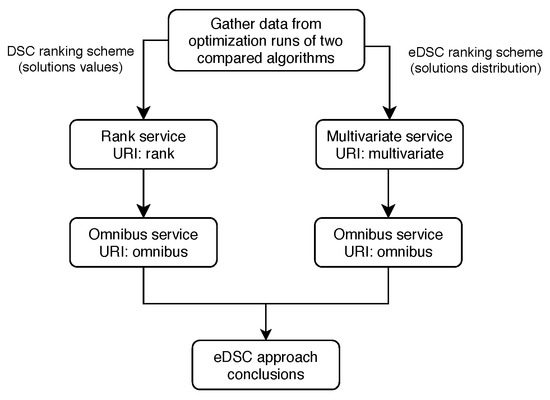
Figure 1.
Extended Deep Statistical Comparison approach.
As we have already mentioned, this analysis consists of two main phases: (i) comparison made with regard to the obtained solutions values (i.e., DSC ranking scheme) and (ii) comparison made with regard to obtained solutions distribution in the search space (i.e., eDSC ranking scheme).
3.1. Comparison Made with Regard to the Obtained Solutions Values (i.e., DSC Ranking Scheme)
The first step in this phase was to use the DSC ranking scheme in order to rank the compared algorithms according to the obtained solutions values on each test instance. For this purpose, the DSCTool rank service was used. For the ranking service, the only decision that should be made was the selection of the statistical test (e.g., KS or AD) that is used to compare the one-dimensional distribution of the obtained solution values and the statistical significance, [18]. In our case, the AD statistical test was selected to be used by the DSC ranking scheme and a statistical significance of 0.05 set. Since we performed the comparison at several time points from the optimization process, the input JSONs for the ranking service should be prepared for each time point. The JSON inputs for the rank service for all pairwise comparisons and all time points from the optimization process can be found at http://cs.ijs.si/dl/dsctool/eDSC-rank.zip. The results of calling the rank service are JSONs that contain DSC rankings for each algorithm pair on every problem instance.
Once the DSC rankings are obtained, the next step is to analyze them using an appropriate omnibus statistical test. In the literature there are a lot of discussions on how to select an appropriate omnibus statistical test [19]. One benefit of using the DSCTool is that the user does not need to take care about this, since the appropriate omnibus statistical test can be selected from the result of the rank service. The DSCTool is an e-Learning tool, so all conditions for selecting an appropriate statistical test have been already checked by the tool and the required statistical knowledge from the user’s side is consequently significantly reduced.
To continue with the analysis, we used the DSCTool omnibus web service. For creating the input JSONs required for the omnibus web service, the results from the rank service were used. Since only two algorithms were compared, the one-sided left-tailed Wilcoxon Signed Rank test was selected, which was proposed by the ranking service. The one-sided left-tailed was selected, since we are interested in if one algorithm performs significantly better and not only if there is a statistical significance between their performances (i.e., two-sided hypothesis). The input JSONs for the omnibus test can be found at http://cs.ijs.si/dl/dsctool/eDSC-rank-omnibus.zip. The omnibus test returns mean DSC rankings for the compared algorithms and p-value, which tells us if the null hypothesis is or is not rejected. In general, if the p-value is lower than our predefined significance level then the null hypothesis is rejected and we can conclude that there is statistical significance between algorithm performances (i.e., the first algorithm has better performance since we are testing one-sided hypothesis). Otherwise, if the p-value is greater or equal then we can conclude that there is no statistical significance between compared algorithms performances.
By performing the first phase of the eDSC approach, we have obtained results for comparing the algorithms with regard to the obtained solutions values using the DSC ranking scheme.
3.2. Comparison Made with Regard to the Distribution of the Obtained Solutions in the Search Space (i.e., eDSC Ranking Scheme)
The second phase involves comparison with regard to the distribution of the obtained solutions in the search space. This requires application of the eDSC ranking scheme. The main difference with the first phase is that we need to use the DSCTool multivariate service instead of the DSCTool rank service. Accordingly, one needs to use actual locations of the solutions when preparing the input JSONs for the multivariate service. This should be done for every pair of algorithms and every time point from the optimization process. The only information that needs to be set in the case of the multivariate service is the distribution preference of the solutions (i.e., clustered or spread) and the statistical significance. In our case, clustered distribution preference has been used and statistical significance of 0.05 set. The JSON inputs for the multivariate service for all pairwise comparisons and every time point from the optimization process can be found at http://cs.ijs.si/dl/dsctool/eDSC-multivariate.zip.
The resulting JSON from the multivariate service has the same structure as the result from the rank service. For this reason, after obtaining the eDSC rankings for every pairwise comparison, they can be further analyzed using the DSCTool omnibus web service (i.e., same as in the first phase). The input JSONs for the omnibus test can be found at http://cs.ijs.si/dl/dsctool/eDSC-multivariate-omnibus.zip.
3.3. Results and Discussion
To provide more information about the exploration and exploitation abilities of the compared algorithms during the optimization process, we compared them in different time points, D*(1000, 10,000, 100,000, and 1,000,000). In Table 2, Table 3, Table 4 and Table 5 the results for eDSC approach are presented for every selected time point, respectively. Each table consists of results obtained by both phases of eDSC approach (i.e., DSC and eDSC ranking scheme) with obtained p-values written in brackets. The results are separated by the | sign. On the left side is the result of comparison between algorithms based on solution values (i.e., DSC ranking scheme), while on the right side is the result for comparison based on solution locations (i.e., eDSC ranking scheme). The / sign represents that the comparison is not logical (i.e., we cannot compare the algorithm with itself), while the + sign indicates that the algorithm written in row significantly outperforms algorithm written in column, while the − sign indicates that the algorithm written in row has statistically significantly worse performance of the algorithm written in column. This interpretation comes from the definition of the null and the alternative hypothesis of the left one-sided test (i.e., : and : , where ’s are sample means of compared algorithms).
Table 2.
Extension of Deep Statistical Comparison (eDSC) analysis at D*1000 function evaluations (FEs).
Table 3.
eDSC analysis at D*10,000 FEs.
Table 4.
eDSC analysis at D*100,000 FEs.
Table 5.
eDSC analysis at max FEs, D*1,000,000.
- D*1000 Function Evaluations:
The Table 2 represents the results for comparing the algorithm performance achieved on D*1000 function evaluations (FEs). In this case, we are primarily interested in the quality of the algorithm performance at the beginning of the optimization, or it can be a case when we have only relatively small number of FEs at our disposal. Looking at the results, it is obvious that DE2 performs significantly better than the other two DE variants (DE1 and DE3) with regard to the solutions quality and their distribution, indicating superior exploration and exploitation abilities. We should point here, that we set the preference of distribution for the eDSC ranking scheme on clustered solutions. Further, DE1 has significantly better exploration and exploitation abilities than DE3, and DE3 performs significantly worse than the the other two DE variants. So if we would had at our disposal only D*1000 evaluations the DE2 is the obvious choice. But if we have more FEs at our disposal, then we do not know if this is the case.
- D*10,000 Function Evaluations:
If we have at our disposal more FEs, then having more clustered distribution of solutions early in the optimization process does not necessary guaranty high quality of solutions later on. If all runs quickly converge to the same area in solution space, one could see this as too quick convergence. In such cases when multimodal search space is explored, the algorithm might be trapped in some local optima. So quick convergence at the beginning of the optimization process is not guaranty of high quality algorithm or its hyperparameters in the long run. Let us look at the Table 3, where results for comparing the algorithm performances achieved on D*10,000 FEs are presented. The DE3 algorithm stayed as the worst performing algorithm, but the relation between the quality of DE1 and DE2 has significantly changed. As we can observe, the preferred distribution of solutions is now significantly better for DE1 algorithm. So seemingly worst initial exploration abilities of DE1 algorithm paid dividends that allowed for achieving significantly better preferred solution distribution. The question that arises is, did we choose the correct preferred distribution when evaluating algorithms at D*1000 FEs? If target FEs would be D*1000 then the selection was correct; however, looking at the results obtained at D*10,000 FEs the answer is not so clear.
- D*100,000 Function Evaluations:
Now let us look at Table 4 and see what happens at D*100,000 FEs. The comparison results stay the same, so no significant changes can be observed between the performances of the algorithms.
- D*1,000,000 Function Evaluations:
Finally, using the Table 5 where the results for comparing the algorithm performances achieved on D*1,000,000 FEs (i.e., the end of the optimization process), it is obvious that the results have changed again. DE3 stayed the worst performing algorithm. The randomly selected hyperparameters for DE3 turned the basic DE into a low performing algorithm (compared to DE1 and DE2) with inefficient exploration abilities, and consequently we cannot say much about exploitation abilities. DE2 significantly worsened its performance compared to DE1 throughout the optimization process, obtaining significantly worse solutions with respect to the solution value and their distribution. The selected hyperparameters worked the best for scenarios when very limited number of FEs are used, but with a higher number of FEs allowed, the performance deteriorated compared to DE1. Finally, the DE1 concluded our analysis as significantly better performing algorithm, that acquired the best solutions with respect to their values and distribution, and showing the best exploration and exploitation abilities among the compared algorithms at D*1,000,000 FEs.
To get a better perception of what is happening during the compared algorithms runs with regard to solutions values and their distribution, a graphical representation of the results for DSC and eDSC ranking schemes is shown in Figure 2 and Figure 3, respectively. On x-axis all time points are represented, while on y-axis, respective rankings of algorithms defined according to results (see Table 2, Table 3, Table 4 and Table 5) of one-sided Wilcoxon Signed Rank test between all compared algorithms are presented (i.e., one means best performance, while three means the worst performance).
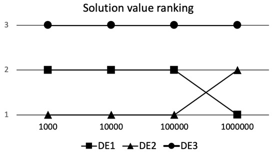
Figure 2.
Deep Statistical Comparison (DSC) ranking.
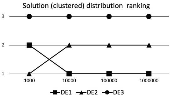
Figure 3.
eDSC ranking.
Finally, we can conclude that the hyperparameters of DE3 are not suitable in any scenario (i.e., time point) since exploration and exploitation performance on our testbed is below the other two DE variants. Next, if we performed the same analysis using experiments with hyperparameters that are in some -neighborhood, we could obtain further information which of the hyperparameters contribute to improving/declining efficiency of exploration and exploitation abilities. The hyperparameters of DE2 provide good initial exploration and exploitation abilities with regard to the other two DE variants. In case when we have scenario with low number of FEs, it is a good starting point to further investigate parameters in some -neighborhood of the DE2 parameters. Such investigation will provide us with information how to further improve the performance in this kind of scenario. Finally, DE1 turned out to be the best performing algorithm when there is a large number of FEs available. Since this is a limited experiment designed to show how we can efficiently use eDSC approach in combination with DSCTool, our conclusions are limited to these three algorithms. If we are comparing different algorithms, this would be enough so one can focus on improving exploration or exploitation abilities of the developed algorithm. In cases when the goal is to understand influence of hyperparameter selection on exploration and exploitation abilities of the algorithm, much more testing would be needed to acquire enough information.
4. Conclusions
One of the most important steps into further development and consequent improvement of new single-objective optimization algorithms is understanding the algorithm’s performance by focusing on the reasons that lead to it. In this paper, we showed how we can easily identify weaknesses and strengths of algorithms’ performances during different stages (e.g., number of solution evaluations) of the optimization process. For this purpose, the DSCTool can help users to make proper statistical analysis quick and error free. Due to its ease of use, the user is able to go through all analysis steps effortlessly by receiving all needed information for performing the analysis. The only important step is the selection of the desired distribution preference of the solutions in the search space (i.e., clustered or spread distributed solutions). As was shown in the experiments, the distribution preference can greatly influence the understanding of the optimization results.
For future work, we would like to extend this analysis focusing on the distribution of population at different time points of the optimization process of single algorithm run, which will provide information about the exploration and exploitation abilities based only on information gathered from solutions in current population, and not compare best solutions between different algorithms runs as it is done here.
Author Contributions
Conceptualization, P.K. and T.E.; methodology, T.E. and P.K.; software, P.K. and T.E.; validation, P.K. and T.E.; formal analysis, T.E. and P.K.; investigation, P.K. and T.E.; writing—original draft preparation, P.K. and T.E.; writing—review and editing, T.E. and P.K.; funding acquisition, T.E. and P.K. All authors have read and agreed to the published version of the manuscript.
Funding
This work was supported by the financial support from the Slovenian Research Agency (research core funding No. P2-0098 and project No. Z2-1867).
Conflicts of Interest
The authors declare no conflict of interest.
Abbreviations
The following abbreviations are used in this manuscript:
| DSC | deep statistical comparison |
| eDSC | extended deep statistical comparison |
| KS | Kolmogorov–Smirnov |
| AD | Anderson–Darling |
| FE | function evaluation |
| DE | differential evolution |
| JSON | JavaScript object notation |
| URI | uniform resource identifier |
References
- Back, T. Evolutionary Algorithms in Theory and Practice: Evolution Strategies, Evolutionary Programming, Genetic Algorithms; Oxford University Press: Oxford, UK, 1996. [Google Scholar]
- Derrac, J.; García, S.; Molina, D.; Herrera, F. A practical tutorial on the use of nonparametric statistical tests as a methodology for comparing evolutionary and swarm intelligence algorithms. Swarm Evol. Comput. 2011, 1, 3–18. [Google Scholar] [CrossRef]
- Wolpert, D.H.; Macready, W.G. No free lunch theorems for optimization. IEEE Trans. Evol. Comput. 1997, 1, 67–82. [Google Scholar] [CrossRef]
- Črepinšek, M.; Liu, S.H.; Mernik, M. Exploration and exploitation in evolutionary algorithms: A survey. ACM Comput. Surv. (CSUR) 2013, 45, 1–33. [Google Scholar] [CrossRef]
- Eftimov, T.; Korošec, P. A Novel Statistical Approach for Comparing Meta-heuristic Stochastic Optimization Algorithms According to the Distribution of Solutions in the Search Space. Inf. Sci. 2019, 489, 255–273. [Google Scholar] [CrossRef]
- Eftimov, T.; Petelin, G.; Korošec, P. DSCTool: A web-service-based framework for statistical comparison of stochastic optimization algorithms. Appl. Soft Comput. 2020, 87, 105977. [Google Scholar] [CrossRef]
- Elhara, O.; Varelas, K.; Nguyen, D.; Tusar, T.; Brockhoff, D.; Hansen, N.; Auger, A. COCO: The Large Scale Black-Box Optimization Benchmarking (bbob-largescale) Test Suite. arXiv 2019, arXiv:1903.06396. [Google Scholar]
- Liang, J.J.; Qu, B.Y.; Suganthan, P.N.; Hernández-Díaz, A.G. Problem Definitions and Evaluation Criteria for the CEC 2013 Special Session on Real-Parameter Optimization; Zhengzhou China and Technical Report; Computational Intelligence Laboratory, Zhengzhou University: Zhengzhou, China; Nanyang Technological University: Singapore, 2013. [Google Scholar]
- Liang, J.J.; Qu, B.Y.; Suganthan, P.N. Problem Definitions and Evaluation Criteria for the CEC 2014 Special Session and Competition on Single Objective Real-Parameter Numerical Optimization; Zhengzhou China and Technical Report; Computational Intelligence Laboratory, Zhengzhou University: Zhengzhou, China; Nanyang Technological University: Singapore, 2014. [Google Scholar]
- Liang, J.J.; Qu, B.Y.; Suganthan, P.N.; Chen, Q. Problem Definitions and Evaluation Criteria for the CEC 2015 Competition on Learning-Based Real-Parameter Single Objective Optimization; Zhengzhou China and Technical Report; Computational Intelligence Laboratory, Zhengzhou University: Zhengzhou, China; Nanyang Technological University: Singapore, 2014. [Google Scholar]
- Hansen, N.; Auger, A.; Brockhoff, D.; Tusar, D.; Tušar, T. COCO: Performance Assessment. arXiv 2016, arXiv:1605.03560. [Google Scholar]
- López-Ibáñez, M.; Dubois-Lacoste, J.; Pérez Cáceres, L.; Stützle, T.; Birattari, M. The irace package: Iterated Racing for Automatic Algorithm Configuration. Oper. Res. Perspect. 2016, 3, 43–58. [Google Scholar] [CrossRef]
- Bartz-Beielstein, T.; Stork, J.; Zaefferer, M.; Rebolledo, M.; Lasarczyk, C.; Ziegenhirt, J.; Konen, W.; Flasch, O.; Koch, P.; Friese, M. Package ‘SPOT’ 2019. Available online: https://mran.microsoft.com/snapshot/2016-08-05/web/packages/SPOT/SPOT.pdf (accessed on 9 June 2016).
- Storn, R.; Price, K. Differential Evolution—A Simple and Efficient Heuristic for Global Optimization over Continuous Spaces. J. Glob. Optim. 1997, 11, 341–359. [Google Scholar] [CrossRef]
- Eftimov, T.; Korošec, P.; Seljak, B.K. A novel approach to statistical comparison of meta-heuristic stochastic optimization algorithms using deep statistics. Inf. Sci. 2017, 417, 186–215. [Google Scholar] [CrossRef]
- Székely, G.J.; Rizzo, M.L. Testing for equal distributions in high dimension. InterStat 2004, 5, 1–6. [Google Scholar]
- Hansen, N.; Finck, S.; Ros, R.; Auger, A. Real-Parameter Black-Box Optimization Benchmarking 2009: Noiseless Functions Definitions; HAL: Lyon, France, 2009. [Google Scholar]
- Eftimov, T.; Korošec, P. The impact of statistics for benchmarking in evolutionary computation research. In Proceedings of the Genetic and Evolutionary Computation Conference Companion, Kyoto, Japan, 15–19 July 2018; pp. 1329–1336. [Google Scholar]
- García, S.; Molina, D.; Lozano, M.; Herrera, F. A study on the use of non-parametric tests for analyzing the evolutionary algorithms’ behaviour: A case study on the CEC’2005 special session on real parameter optimization. J. Heuristics 2009, 15, 617. [Google Scholar] [CrossRef]


© 2020 by the authors. Licensee MDPI, Basel, Switzerland. This article is an open access article distributed under the terms and conditions of the Creative Commons Attribution (CC BY) license (http://creativecommons.org/licenses/by/4.0/).