The Singular Value Decomposition over Completed Idempotent Semifields

Abstract

In this paper, we provide a basic technique for Lattice Computing: an analogue of the Singular Value Decomposition for rectangular matrices over complete idempotent semifields (i-SVD). These algebras are already complete lattices and many of their instances—the complete schedule algebra or completed max-plus semifield, the tropical algebra, and the max-times algebra—are useful in a range of applications, e.g., morphological processing. We further the task of eliciting the relation between i-SVD and the extension of Formal Concept Analysis to complete idempotent semifields ($\mathcal{K}$-FCA) started in a prior work. We find out that for a matrix with entries considered in a complete idempotent semifield, the Galois connection at the heart of $\mathcal{K}$-FCA provides two basis of left- and right-singular vectors to choose from, for reconstructing the matrix. These are join-dense or meet-dense sets of object or attribute concepts of the concept lattice created by the connection, and they are almost surely not pairwise orthogonal. We conclude with an attempt analogue of the fundamental theorem of linear algebra that gathers all results and discuss it in the wider setting of matrix factorization.

1. Introduction

Lattice Computing (LC) [1] intends to provide “an evolving collection of tools and methodologies that process lattice-ordered data”, as a means of establishing an information processing paradigm belonging to the wider field of Computational Intelligence [2], with explicit aim at modelling Cyber Physical Systems [3].

In this paper, we present a fundamental tool for the factorization of matrices by developing the Singular Value Decomposition (SVD), a staple technique of data analysis [4,5], for matrices over idempotent semifields [6,7]. In it we both use computing in lattices—since the matrices take values in idempotent semifield, an algebraic structure which is similar, but distinct to a fuzzy semiring—and computing with lattices—since our results highlight the role of the lattices of Formal Concept Analysis (FCA) [8] in reconstructing matrices.

1.1. Motivation

For that purpose, consider a linear form between spaces $R:Y\to X$ and its adjoint $R^{⊛}:X\to Y$. It is extremely interesting to be able to describe these transformations as simply as possible—e.g., ideally with diagonal matrices—but to do so we have to specify further the algebras in which such linear forms can be represented and computed with.

A generalization of the properties of standard matrices over fields shows that a sensible point to start from are commutative semirings that already have the addition and multiplication operators to carry out matrix-vector operation (Section 2.1). The diagram of Figure 1 sketches the organization of commutative semirings (cfr. [9] (Figure 2); see also Section 2.1.1). However, generic semirings are too abstract and do not have many tools to work with. One thing we can do, though, is to suppose that the spaces are free, so that the domain and range spaces are products of copies of the basic semifield $Y\equiv K^m$ and $X\equiv K^g$. We treat all vectors as columns (that is, right semi-vector spaces) so that the linear forms above can be represented as matrices in these $R\in K^{g\times m}$ and $R^{⊛}\in K^{m\times g}$.

To go on specifying these forms, it is well known that the most important distinction between semirings is whether the semiring has an additive group structure or not [10,11]: additively cancellative semirings and zerosumfree semirings are as far apart as algebras can be in this respect.

Figure 1 shows, actually, a concept lattice of the position of positive semifields within the commutative semirings, as well as the better known collateral families of fields such as $\mathbb{R}$ and distributive lattices such as $\langle [0,1],max,min\rangle$.

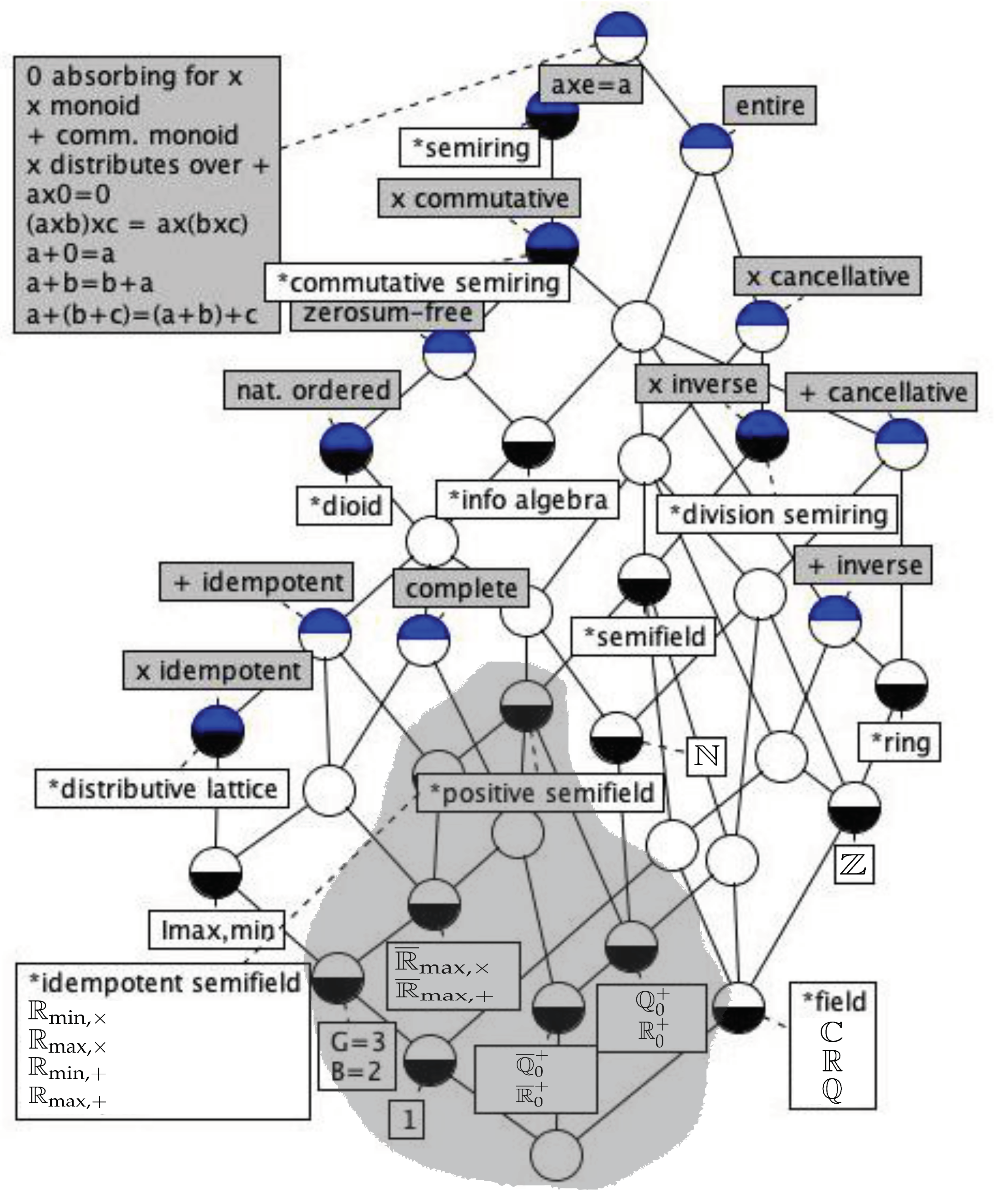
• If we can guarantee the existence of additive inverses, several further observations might eventually lead us to work in the familiar landscape of the groups such as $\mathbb{Z}$ and modules.
• On the other hand, if we cannot guarantee the existence of additive inverses, the toolset is quite scarce. It is first improved by demanding a natural order compatible with the operations in the semiring, leading to dioids (for double monoids), or entireness, leading to so-called information algebras.

However, the step that enormously increases the toolset is to accept the existence of the multiplicative inverse that transforms the semiring into a semifield (see Section 2.1).

• Adding the semifield structure to a group eventually leas us to the fields such as $\mathbb{R}$ or $\mathbb{C}$ and vector spaces of standard algebra.
  In this case, the SVD is a well-known decomposition scheme for matrices over a standard field, e.g., real or complex numbers [4] which clarifies enormously the action of the linear form (Section 1.2).
• On the other hand, adding the semifield structure to information algebras that are dioids leads us to positive semifields and their positive semimodules, which are quite varied.

To the extent of our knowledge, the only well-developed theory concerns a subset of the positive semifields, the complete idempotent semifields and their semimodules, the ones we will be using in this paper (Section 2.1.2, Section 2.1.3, Section 2.1.4, Section 2.1.5 and Section 2.1.6). Idempotent semifields are important for us because we are putting forth the idea that to understand the spaces of linear transformations in idempotent semifields, FCA ([8], and Section 1.4 below) and in general Galois connections [12] (see also Appendix B) are needed.

1.2. The Singular Value Decomposition

Readers familiar with the SVD may skip this section.

Before turning to idempotent semifields and their lattices, let us recall that if the semifields are actually “complete” fields, e.g., $\overline{\mathcal{K}}\equiv \mathbb{R}$ or $\overline{\mathcal{K}}\equiv \mathbb{C}$, Lanczos [13] shows how to aggregate the two linear forms into a single eigenvalue problem to carry out the (standard) SVD of R (and $R^{⊛}$).

Theorem 1.

Let $\overline{\mathcal{K}}$ be $\mathbb{R}$ or $\mathbb{C}$. Given a matrix $A\in {\mathcal{M}}_{m\times n}(\overline{\mathcal{K}})$ representing a linear form between the spaces $\mathcal{X}\equiv {\overline{\mathcal{K}}}^n$ and $\mathcal{Y}\equiv {\overline{\mathcal{K}}}^m$, and $A^{⊛}$ its adjoint. We define the following subspaces of $\mathcal{X}$ and $\mathcal{Y}$:

• The image, range or column space of A, $\mathrm{I}\mathrm{M}\left(A\right)\subseteq \mathcal{Y}$ as $\mathrm{I}\mathrm{M}\left(A\right)=\{Ax\mid x\in \mathcal{X}\}$,
• The kernel or null-space of A, $\mathrm{K}\mathrm{ER}(A)\subseteq \mathcal{X}$, as $\mathrm{K}\mathrm{ER}(A)=\{x\in \mathcal{X}\mid Ax=0_{\mathcal{Y}}\}$,
• The co-image or row space of A, $\mathrm{I}\mathrm{M}\left(A^{⊛}\right)\subseteq \mathcal{X}$, as $\mathrm{I}\mathrm{M}\left(A^{⊛}\right)=\{A^{⊛}y\mid y\in \mathcal{Y}\}$,
• The co-kernel or left null-space of A, $\mathrm{K}\mathrm{ER}(A^{⊛})\subseteq \mathcal{Y}$, as $\mathrm{K}\mathrm{ER}(A^{⊛})=\{y\in \mathcal{Y}\mid A^{⊛}y=0_{\mathcal{X}}\}$.

Then:

1.

From $\mathrm{I}\mathrm{M}\left(A^{⊛}\right)$ to $\mathrm{I}\mathrm{M}\left(A\right)$, the matrix yields an invertible transformation wherefore they have the same dimension, the rank, $r=dim\mathrm{I}\mathrm{M}\left(A\right)=dim\mathrm{I}\mathrm{M}\left(A^{⊛}\right).$

2.

In $\mathcal{X}$, the kernel is the orthogonal complement of the co-image, $\mathrm{K}\mathrm{ER}(A)=\mathrm{I}\mathrm{M}{\left(A^{⊛}\right)}^{\perp }$.

3.

In $\mathcal{Y}$, the co-kernel is the orthogonal complement of the co-image, $\mathrm{K}\mathrm{ER}(A^{⊛})=\mathrm{I}\mathrm{M}{\left(A\right)}^{\perp }$

4.

(Rank-nullity theorem) The dimension of the domain space decomposes as: $dim\mathrm{I}\mathrm{M}\left(A^{⊛}\right)+dim\mathrm{K}\mathrm{ER}(A)=dim\mathcal{X}$.

5.

(Rank-co-nullity) The dimension of the range space decomposes as: $dim\mathrm{I}\mathrm{M}\left(A\right)+dim\mathrm{K}\mathrm{ER}(A^{⊛})=dim\mathcal{Y}$.

6.

there is a factorization $A=U\mathsf{\Sigma }{V}^{⊛}$ given in term of three matrices

(a)

$U\in {\mathcal{M}}_{m\times m}(\mathcal{K})$ is a unitary matrix of left singular vectors.

(b)

$\mathsf{\Sigma }\in {\mathcal{M}}_{m\times n}(\mathcal{K})$ is a diagonal matrix of non-negative real values called the singular values.

(c)

$V\in {\mathcal{M}}_{n\times n}(\mathcal{K})$ is a unitary matrix of right singular vectors, and they can be structured as:

$$\begin{array}{cccccc}\hfill U& =\left(\begin{array}{c}{U}_1{U}_0\end{array}\right)\hfill & \hfill \mathsf{\Sigma }& =\left(\begin{array}{cc}{\mathsf{\Sigma }}_1& 0\\ 0& {\mathsf{\Sigma }}_0\end{array}\right)\hfill & \hfill V& =\left(\begin{array}{c}{V}_1{V}_0\end{array}\right)\hfill \end{array}$$

(1)

where ${\mathsf{\Sigma }}_0$ is a zero matrix and $U_0$ and $V_0$ are the left and right singular vectors, respectively, of the null singular value, if it exists.

7.

And conjugate-dually, there is a factorization of $A^{⊛}$ in terms of the same three matrices

$$A^{⊛}=V{\mathsf{\Sigma }}^{⊛}{U}^{⊛}$$

where image and co-image, kernel and co-kernel swap roles.

An excellent but very brief summary of the affordances of SVD, integrated with the fundamental theorem of linear algebra between vector spaces, without the technical encumbrance, is [14] from which Theorem 1 is synthesized—see the figures therein for abstract representations of spaces. A very interesting approach tying the linear transformations and spectral considerations for understanding their associated subspaces is [13]: both have inspired material in this paper. A modern, computer-oriented exposition of the SVD can be found in [4].

Note that A can also be written using outer products in terms of the singular value ${\sigma }_i$ and its corresponding singular vectors $(u_i,v_i)$ as:

$$\begin{array}{c}\hfill A=\sum _{i=1}^{min(m,n)}{\sigma }_i{u}_i{v}_i^{*}\end{array}$$

(2)

hence, since the SVD is a costly procedure, it is also interesting to find $k\le min(m,n)$ such that using the k greatest singular values we may approximate:

$$\begin{array}{c}\hfill A\approx \sum _{i=1}^k{\sigma }_i{u}_i{v}_i^{*}.\end{array}$$

(3)

In particular, singular vectors of the null eigenvalue never contribute to the reconstruction so they may be discarded.

Note also that this tool is particularly useful in applications in data analysis such as Latent Semantic Analysis [15] or Principal Component Analysis [16]. The book [17] explains some of its applications.

1.3. Formal Concept Analysis and Boolean Matrix Factorization

Consider a set of formal objects G and a (disjoint) set of formal attributes M. A matrix $I\in K^{G\times M}$ with entries in a set K with object-indexed rows and attribute-indexed columns and is a ubiquitous object in mathematical applications ranging from the theory of vector spaces in pure Mathematics [14], to datasets in statistics [18], to measurement theory in general Science.

When the support set is $2=\{0,1\}$ and carries a Boolean algebra, Wille [19] had the intuition to coalesce these objects, attributes and relationship in the guise of a “formal context” $(G,M,I)$, with $I\in 2^{G\times M}$, and proposed Formal Concept Analysis (FCA) against the backdrop of Order Theory [8]. This is about describing special pairs of sets of objects and attributes called the formal concepts and their properties as defined by the formal context. We next state an extended form of the basic theorem.

Theorem 2

(Fundamental theorem of FCA). Let G be a set of formal objects, M a set of formal attributes and $(G,M,I)$ be a formal context with $I\subseteq G\times M$. Then:

1.

The context analysis phase.

(a)

The polar operators of the context ${·}^{\uparrow }:2^G\to 2^M$ and ${·}^{\downarrow }:2^M\to 2^G$.

$$\begin{array}{cccc}\hfill A^{\uparrow }& =\{m\in M\mid \forall g\in A,gIm\}\hfill & \hfill B^{\downarrow }& =\{g\in G\mid \forall m\in B,gIm\}\hfill \end{array}$$

form a Galois connection $({·}^{\uparrow },{·}^{\downarrow }):2^G⥎2^G$ whose formal concepts are the pairs $(A,B)$ of closed elements such that $A^{\uparrow }=B\iff A=B^{\downarrow }$ whence the set of formal concepts is

$$\mathfrak{B}(G,M,I)=\{(A,B)\in 2^G\times 2^M\mid A^{\uparrow }=B\iff A=B^{\downarrow }\}.$$

(b)

Formal concepts are partially ordered with the hierarchical order

$$(A_1,B_1)\le (A_2,B_2)\iff A_1\subseteq A_2\iff B_1\supseteq B_2.$$

and the set of formal concepts with this order $\langle \mathfrak{B}(G,M,I),\le \rangle$ is a complete lattice $\underline{\mathfrak{B}}(G,M,I)$ called the concept lattice of $(G,M,I)$.

(c)

In $\underline{\mathfrak{B}}(G,M,I)$ infima and suprema are given by:

$$\begin{array}{cccc}\hfill \underset{t\in T}{\bigwedge }(A_t,B_t)& =\left(\bigcap _{t\in T}{A}_t,{\left(\bigcap _{t\in T}{A}_t\right)}^{\uparrow }\right)\hfill & \hfill \underset{t\in T}{\bigvee }(A_t,B_t)& =\left({\left(\bigcap _{t\in T}{B}_t\right)}^{\downarrow },\bigcap _{t\in T}{B}_t\right)\hfill \end{array}$$

(4)

(d)

The basic functions $\overline{\gamma }:G\to V$ and $\overline{\mu }:M\to V$

$$\begin{array}{cccc}\hfill g& \mapsto \overline{\gamma }(g)=({\{g\}}^{\uparrow \downarrow },{\{g\}}^{\uparrow })\hfill & \hfill m& \mapsto \overline{\mu }(m)=({\{m\}}^{\downarrow },{\{m\}}^{\downarrow \uparrow })\hfill \end{array}$$

are mappings such that $\overline{\gamma }(G)$ is supremum-dense in $\underline{\mathfrak{B}}(G,M,I)$, $\overline{\mu }(M)$ is infimum-dense in $\underline{\mathfrak{B}}(G,M,I)$.

2.

The context synthesis phase.

(a)

A complete lattice $\mathbb{L}=\langle L,\le \rangle$ is isomorphic to (read can be built as) the concept lattice $\underline{\mathfrak{B}}(G,M,I)$ if and only if there are mappings $\overline{\gamma }:G\to L$ and $\overline{\mu }:M\to L$ such that

• $\overline{\gamma }(G)$ is supremum-dense in $\mathbb{L}$, $\overline{\mu }(M)$ is infimum-dense in $\mathbb{L}$, and
• $gIm$ is equivalent to $\overline{\gamma }(g)\le \overline{\mu }(m)$ for all $g\in G$ and all $m\in M$.

(b)

In particular, consider the doubling context of $\mathbb{L}$, $K(\mathbb{L})=(L,L,\le )$, and the standard context of $\mathbb{L}$, $S(\mathbb{L})=(J(\mathbb{L}),M(\mathbb{L}),\le )$ where $J(\mathbb{L})$ and $M(\mathbb{L})$ are the sets of join- and meet-irreducibles, respectively, of $\mathbb{L}$, then

$$\underline{\mathfrak{B}}(K(\mathbb{L}))\cong \mathbb{L}\cong \underline{\mathfrak{B}}(S(\mathbb{L})).$$

Proof. 

See Chapter 1 of [8], or the slow buildup of results in Chapter 7 of [20]. □

Previously, Birkhoff [21] and Ore [22] investigated the notion of Galois connection, and Barbut and Monjardet [23,24] came up with the notion of the “Galois lattice”—essentially the concept lattice—of a binary relation.

Note that FCA can both be understood as a data analysis technique for Boolean tables—the analysis phase—and as a synthesis technique for a Boolean matrix that “respects” the order of some lattice—the synthesis phase. For the purpose of developing a SVD, the synthesis phase is the more important step. However, since the core of this phase is to conform the Boolean matrix so that its concept lattice—issued from the analysis phase—is isomorphic to the lattice being used as guide, both phases seem to be equally important.

If a pair $(A,B)\in \mathfrak{B}(G,M,I)$ is a formal concept, then we say A is its extent and B is its intent. An early result of the relevance of FCA for for Boolean Matrix Factorization (BMF) was first described in [25]:

Theorem 3

(Theorem 1 of [25], adapted). Let G be a set of formal objects $\left|G\right|=g$, M a set of formal attributes $\left|M\right|=m$ and $(G,M,I)$ be a formal context with $I\subseteq G\times M$. If $I=A\circ B$ for $A\in 2^{g\times k}$ and $B\in 2^{k\times m}$ where the multiplication is that of Boolean matrices, then there exists $F\subseteq \mathfrak{B}(G,M,I)$ with $\left|F\right|\le k$ such that for the Boolean matrices $A_F\in 2^{g\times \left|F\right|}$ and $B_F\in 2^{\left|F\right|\times m}$ we have $I=A_F\circ B_F$.

So if a Boolean matrix accepts a BMF, it accepts one in terms of formal concepts with, possibly, even less factors. The expansion of the matrix operation leads to further understanding of this issue:

$$\begin{array}{cc}\hfill I& =\underset{f\in F}{\bigvee }{A}_{·f}\circ B_{f·}\hfill \end{array}$$

where we use the dot to range over all the indices in a line (row, column) of the matrix. This induces two observations:

• The operations invoked on the matrix depend on the underlying algebra carried by $22$, e.g., a Boolean algebra, and suggests there might be a reconstruction for every algebra definable on that carrier set. Since it is well-known that the most abstract structure to support matrix algebra is that of a semiring, we review in Section 2.1 several concepts around semirings.
  The Boolean algebra is embedded in every idempotent semifield, a special kind of semiring with an idempotent addition (Section 2.1–Section 2.1.2), and similar results for the reconstruction of matrices have been proven [26]. This paper is a natural extension of those results.
• Clearly, $A_{·f}$ and $B_{f·}$ are the extent and intent of formal concepts encoded in correlative columns of $A_F$ and rows of $B_F$, and the ∘ operation is an external product, which suggests that extents and intents are being used as column and row vectors, respectively, if both were used as column vectors, the factorization would have to be written as $I=A_F\circ B_F^{\mathrm{T}}$. This points to the fact that the concepts of Linear Algebra over semirings, in general are important for this Theorem 3.

1.4. Formal Concept Analysis as Linear Algebra over Idempotent Semifields

There is another extension to FCA called $\mathcal{K}$-FCA where the entries in the incidence belong to a complete idempotent semifield $\overline{\mathcal{K}}$ [27,28,29]. An idempotent semifield is an algebra that resembles a standard field but whose additive structure is idempotent and thus has no inverse [10], instead it exhibits strong order-related properties [11]. One of the best known examples of this structure is the completed max-plus algebra [6], by other names minimax algebra [30], morphological algebra [31] or lattice algebra [32].

In [33] it was proven that $\mathcal{K}$-FCA is best understood in terms of the linear algebra of the semivector spaces over $\overline{\mathcal{K}}$ (see Section 2.1). This was later extended in [34] in the sense of better interpreting the analogues of the kernels of the linear transformation R and properly describing FCA itself as a special case of $\mathcal{K}$-FCA.

Unfortunately, “natural” positive semifields are incomplete—barring the Boolean semifield $\mathbb{B}$—lacking an inverse for the bottom element in the order, and the top completion provides not one but a pair of dually ordered semifields $(\overline{\mathcal{K}},\underline{\mathcal{K}})$ with the inversion in the multiplicative group acting as the duality inducing operator. This entails that expressions will have two (differently completed) multiplications, additions, etc., causing a notational problem which has not yet been agreed upon in the community (see Appendix A). This is precisely the notational problem made evident by Moreau [35] for convex analysis, whose dotted notation we adopt throughout (see Section 2.1.3).

Once the notational problem is solved, this investigation leads naturally to highlight not only the Galois connection of (standard) FCA as expressed in Theorem 2, but other three types of Galois connection established by matrices (see Appendix B and [12]) which can also be understood as Galois connections between semimodules over idempotent semifields, the analogues of vector spaces over fields (Section 2.1.3, Section 2.1.4, Section 2.1.5 and Section 2.1.6). We call this construction the 4-fold $\mathcal{K}$-FCA [36] and this is the core of our approach to integrating the i-SVD into $\mathcal{K}$-FCA(see Section 2.2).

Furthermore, we have not specified which of the two semifields—that with the above-dotted or the one with the below-dotted operations—is “the reference”. We typically consider that the below-dotted reference is for semifields whose order aligns with the usual order in $\langle \mathbb{R},\le \rangle$ and this is the one we call $\overline{\mathcal{K}}$, because it is completed with a top element, so if $K=\mathbb{R}\cup \{-\infty \}$, then $\overline{\mathcal{K}}=\mathbb{R}\cup \{\pm \infty \}$. Changing this semifield to its order-dual $\underline{\mathcal{K}}$ is what we call changing the bias of the analysis (see results in Section 2.2.3). It has important repercussions because it changes the way the matrix is approximated in the i-SVD (see Section 3).

1.5. Previous Results for the SVD over Idempotent Semifields

To the best of our knowledge, the first and foremost attempt at define an i-SVD for rectangular matrices over the max-plus algebra is [37]. The authors have a long tradition of using spectral results in their papers [31,38,39], but we know of no direct application of the SVD after their initial paper, nor the embedding of the construction in the wider setting of Galois connections.

A related result was obtained over the symmetrized max-plus semiring in [40] and later revisited in [41], but it is not directly applicable to our problem. They were, however, used to solve the related problem of finding the singular values of a matrix over the (incomplete) max-plus semiring, using the technique of logarithmic-exponential transformation between the standard eigenvalue and max-plus eigenvalue problems [42].

1.6. Reading Guide

This paper is an updated and completed version of [26] using ideas from [36]. In it, we investigate:

(1)

An idempotent analogue of the SVD based on the irreducibles of a Galois connection,

(2)

What are the implications of a change of bias, i.e., using $\underline{\mathcal{K}}$ for the analysis, and

(3)

Whether there is and analogue of a Fundamental Theorem of Linear Algebra for matrices over idempotent semifields.

For that purpose, we first review $\mathcal{K}$-FCA in Section 2 including the notation and maths of completed idempotent semifields that allows us to define the different connections and, in particular, the i-SVD on the Galois connection. Then we present our results in Section 3, prior to discussing them vis-à-vis similar solutions in Section 4.

2. Preliminaries

2.1. Linear Algebra over Complete Idempotent and Positive Semifields

2.1.1. A Short Systemization

A semiring is an algebra $\mathcal{S}=\langle S,\oplus ,\otimes ,ϵ,e\rangle$ whose additive structure, $\langle S,\oplus ,ϵ\rangle$, is a commutative monoid and whose multiplicative structure, $\langle S\backslash \{ϵ\},\otimes ,e\rangle$, is a monoid with multiplication distributing over addition from right and left and with additive neutral element absorbing for ⊗, i.e., $\forall a\in S,ϵ\otimes a=ϵ$.

A commutative semiring is one whose multiplicative law is commutative. Note that semirings can be primitive or constructed from other algebras: although the base semiring is commutative, the construction may not as in the example below.

Example 1

(Square matrices semirings). Given a semiring $\mathcal{S}$, the semiring of square matrices of order n over $\mathcal{S}$ is the structure ${\mathcal{M}}_n(\mathcal{S})=\langle S^{n\times n},+,\times ,0,E\rangle$ where + is the usual entry-wise addition, × is usual matrix multiplication, 0 is the matrix whose entries are all the zero in $\mathcal{S}$ and E that matrix whose entries are all zero except at the diagonal, where they are the unit in $\mathcal{S}$. Note that the operations for matrix addition and multiplication are those of the underlying semiring $\mathcal{S}$ whence this construction is completely generic.

All basic semirings in this paper are commutative, except for the example above, an important example of non-commutative semiring. Many more examples can be found in [10].

For the systematization of semirings the important operation seems to be addition [10,11]. In particular, every semiring accepts a canonical preorder, $a\le b$ if and only if there exists $c\in D$ with $a\oplus c=b$. A dioid is a semiring $\mathcal{D}$ where this relation is actually an order that is compatible with multiplication and addition, e.g., if $a\le b$ then for all $c\in S$ still holds $a\otimes c\le b\otimes c$ and $a\oplus c\le b\oplus c$. Dioids are zerosumfree, i.e., they have no non-null additive factors of zero. In this, dioids are as different as a semiring can be from a ring, a quality suggested by their distance in the lattice of semirings and their properties of Figure 1.

A semiring $\mathcal{S}$ is complete, if for any index set I including the empty set, and any ${\{a_i\}}_{i\in I}\subseteq \mathcal{S}$ the (possibly infinite) summations ${\sum }_{i\in I}{a}_i$ are defined and the distributivity conditions: $\left({\sum }_{i\in I}{a}_i\right)\otimes c={\sum }_{i\in I}\left(a_i\otimes c\right)$ and $c\otimes \left({\sum }_{i\in I}{a}_i\right)={\sum }_{i\in I}\left(c\otimes a_i\right)$, are satisfied. Note that for $c=e$ the above demand that infinite sums have a result. Commutative complete dioids are already complete residuated lattices.

An idempotent semiring is a dioid whose addition is idempotent, examples of which are:

Example 2

(Idempotent semirings).

• The Boolean lattice $\mathbb{B}=\langle \{0,1\},\vee ,\wedge ,0,1\rangle$
• All fuzzy semirings, e.g., $\langle [0,1],max,min,0,1\rangle$
• The min-plus semiring or tropical algebra ${\mathbb{R}}_{min,+}=\langle \mathbb{R}\cup \{\infty \},min,+,\infty ,0\rangle$ also called the optimization algebra.
• The max-plus semiring or polar algebra ${\mathbb{R}}_{max,+}=\langle \mathbb{R}\cup \{-\infty \},max,+,-\infty ,0\rangle$ also called the schedule algebra.

Of the semirings above, only the boolean lattice and the fuzzy semirings are complete dioids, since the rest lack the greatest element in the order, the top ⊤.

A semiring is a semifield if there exists a multiplicative inverse for every element $a\in S$, notated as $a^{-1}$, except, possibly, for the null element. Semifields are all entire, i.e., they have no non-null factors of the zero element. Note that there is an infinite quantity of semifields (see Chapter 8 of [11], Sections 4.4.3 and 4.4.4).

A semifield that is also a dioid is called a positive semifield, so these have all a natural order compatible with addition and multiplication (see Figure 1). If its addition is furthermore idempotent it is called an idempotent semifield.

Example 3

(Positive and idempotent semifields).

1.

The non-negative rationals ${\mathbb{Q}}_{\ge 0}$ and non-negative reals ${\mathbb{R}}_{\ge 0}$ are two positive semifields.

2.

The min-plus and max-plus algebras of Example 2 are idempotent semifields.

3.

The min-times algebra ${\mathbb{R}}_{min,\times }=\langle \mathbb{R}\cup \{\infty \},min,\times ,\infty ,1\rangle$ and the max-times algebra ${\mathbb{R}}_{max,\times }=\langle \mathbb{R},max,\times ,0,1\rangle$ are also idempotent semifields.

2.1.2. Semifield Completions

As noted above, positive semifields are incomplete in their natural order, lacking an adequate inverse for the bottom in the order, but there are procedures for completing such structures [29] (Construction 1) and we will not differentiate between complete or completed structures. This construction actually obtains a pair of dually ordered complete positive semifields from a single (incomplete) positive semifield. Its results are collected below as a Theorem.

Theorem 4.

For every (incomplete) positive semifield $\mathcal{K}=\langle K,\oplus ,\otimes ,{·}^{-1},\perp ,e\rangle$

1.

There is a pair of completed semifields over $\overline{K}=K\cup \{\top \}$

$$\begin{array}{cccc}\hfill \overline{\mathcal{K}}& =\langle K,\underset{\mathbf{\dot{}}}{\oplus },\underset{\mathbf{\dot{}}}{\otimes },{·}^{-1},\perp ,e,\top \rangle \hfill & \hfill {\overline{\mathcal{K}}}^{-1}& =\langle K,\dot{\oplus },\dot{\otimes },{·}^{-1},\top ,e,\perp \rangle \hfill \end{array}$$

(5)

where $\top ={\perp }^{-1}$ and $\perp ={\top }^{-1}$ by definition,

2.

In addition to the individual laws as positive semifields, we have the modular laws:

$$\begin{array}{cccc}\hfill (u\underset{\mathbf{\dot{}}}{\oplus }v)\underset{\mathbf{\dot{}}}{\otimes }(u\dot{\oplus }v)& =u\underset{\mathbf{\dot{}}}{\otimes }v\hfill & \hfill (u\underset{\mathbf{\dot{}}}{\oplus }v)\dot{\otimes }(u\dot{\oplus }v)& =u\dot{\otimes }v\hfill \end{array}$$

(6)

the analogues of the De Morgan laws:

$$\begin{array}{cccc}\hfill u\underset{\mathbf{\dot{}}}{\oplus }v& ={(u^{-1}\dot{\oplus }{v}^{-1})}^{-1}\hfill & \hfill u\dot{\oplus }v& ={(u^{-1}\underset{\dot{}}{\oplus }{v}^{-1})}^{-1}\hfill \\ \hfill u\underset{\mathbf{\dot{}}}{\otimes }v& ={(u^{-1}\dot{\otimes }{v}^{-1})}^{-1}\hfill & \hfill u\dot{\otimes }v& ={(u^{-1}\underset{\dot{}}{\otimes }{v}^{-1})}^{-1}\hfill \end{array}$$

(7)

and the self-dual inequality in the natural order

$$\begin{array}{c}\hfill u\underset{\mathbf{\dot{}}}{\otimes }(v\dot{\otimes }w)\preccurlyeq (u\underset{\mathbf{\dot{}}}{\otimes }v)\dot{\otimes }w.\end{array}$$

(8)

3.

Furthermore, if $\mathcal{K}$ is a positive dioid, then the inversion operation is a dual order isomorphism between the dual order structures $\overline{\mathcal{K}}=\langle K,\preccurlyeq \rangle$ and ${(\overline{\mathcal{K}})}^{-1}=\langle K,\succcurlyeq \equiv {\preccurlyeq }^{\delta }\rangle$ with the natural order of the original semifield a suborder of the first structure.

Several points need to be explicited regarding this theorem:

• The issue of notation is contentious: so as not to derail the exposition, in Appendix A we discuss the problem and our decisions, which essentially amount to using a notation that maximally resembles that of linear algebra but also accommodates Boolean algebra.
• Please also note that in complete semifields $e\ne \top$ which distinguishes them from inclines, and also that the inverse for the null is prescribed as ${\perp }^{-1}=\top$. On a practical note, residuation in complete commutative idempotent semifields can be expressed in terms of inverses, and this extends to eigenspaces, examples of which will be given in the following sections.
• In fact, complete idempotent semifields $\overline{\mathcal{K}}=\langle K,\underset{\dot{}}{\oplus },\dot{\oplus },\underset{\dot{}}{\otimes },\dot{\otimes },{·}^{-1},\perp ,e,\top \rangle$, appear as enriched structures, the advantage of working with them being that meets can be expressed by means of joins and inversion as $a\dot{\oplus }b={(a^{-1}\underset{\mathbf{\dot{}}}{\oplus }{b}^{-1})}^{-1}$.

They will be the main algebras used in this paper, so we next present their best known instances.

Example 4

(Complete idempotent semifields). This example gathers the most important subjects of investigation. These are all completed idempotent semifields that come in dual pairs.

1.

The “smallest” example of complete idempotent semifield is $\mathbb{B}\cong 22$, but it lacks a common neutral element for multiplications $\underset{\mathbf{\dot{}}}{\otimes }$ and $\dot{\otimes }$.

2.

The next smallest is $33=\langle \{\perp ,e,\top \},\underset{\dot{}}{\oplus },\dot{\oplus },\underset{\dot{}}{\otimes },\dot{\otimes },\perp ,e,\top \rangle .$$22$ is embedded in $33$, and $33$ is embedded in any bigger complete semifield.

3.

The complete max-times semifield ${\overline{\mathbb{R}}}_{min,\times }=\langle [0,\infty ],max,\underset{\mathbf{\dot{}}}{\times },{·}^{-1},\perp =0,1,\top =\infty \rangle$

4.

The complete min-times semifield ${\overline{\mathbb{R}}}_{min,\times }=\langle [0,\infty ],min,\dot{\times },{·}^{-1},{\perp }^{-1}=\infty ,1,{\top }^{-1}=0\rangle$

5.

The complete min-plus semifield ${\overline{\mathbb{R}}}_{min,+}=\langle \mathbb{R}\cup \{-\infty ,\infty \},min,\dot{+},-·,\infty ,0\rangle$.

6.

The complete max-plus semifield ${\overline{\mathbb{R}}}_{max,+}=\langle \mathbb{R}\cup \{-\infty ,\infty \},max,\underset{\mathbf{\dot{}}}{+},-·,-\infty ,0\rangle$.

Note that the completed tropical algebra ${\overline{\mathbb{R}}}_{min,+}$ and the completed schedule algebra ${\overline{\mathbb{R}}}_{max,+}$ are the algebras in Convex Analysis [35], Morphological Analysis [43], and Idempotent Analysis [11]. In them we have $\forall c\in [-\infty ,\infty ],-\infty \underset{\dot{}}{+}c=-\infty$ and $\infty \dot{+}c=\infty$, which solves several issues in simultaneously handling both semifields. These are the concrete algebras that we use as prototypes of completed idempotent semifields.

Although idempotent complete semifields may look like a very restricted catalogue, there are infinite positive complete semifields [9].

2.1.3. Idempotent Semimodules

Let $\mathcal{D}=\langle D,+,\times ,{ϵ}_D,e_D\rangle$ be a commutative semiring. A $\mathcal{D}$-semimodule $\mathcal{X}=\langle X,\oplus ,\odot ,{ϵ}_X\rangle$ is a commutative monoid $\langle X,\oplus ,{ϵ}_X\rangle$ endowed with a scalar action $(\lambda ,x)\mapsto \lambda \odot x$ satisfying the following conditions for all $\lambda ,\mu \in D$, $x,x^{\prime }\in X$:

$$\begin{array}{cccc}\hfill (\lambda \times \mu )\odot x& =\lambda \odot (\mu \odot x)\hfill & \hfill \lambda \odot (x\oplus x^{\prime })& =\lambda \odot x\oplus \lambda \odot x^{\prime }\hfill \\ \hfill (\lambda +\mu )\odot x& =\lambda \odot x\oplus \mu \odot x\hfill & \hfill \lambda \odot {ϵ}_X& ={ϵ}_X={ϵ}_D\otimes x\hfill \\ \hfill e_D\odot x& =x\hfill \end{array}$$

(9)

If $\mathcal{D}$ is commutative, idempotent or complete, then $\mathcal{X}$ is also commutative, idempotent or complete.

Recall the semiring of square matrices of Example 1. The following defines the matrix semimodules.

Example 5

(Finite matrix semimodules [29]). For $n,p\in \mathbb{N}$, the semimodule of finite matrices ${\mathcal{M}}_{n\times p}(\mathcal{S})=\langle S^{n\times p},\oplus ,\mathcal{E}\rangle$ is a $({\mathcal{M}}_n(\mathcal{S}),{\mathcal{M}}_p(\mathcal{S}))$-bisemimodule [10], with matrix multiplication-like left and right actions and entry-wise addition. Note that $E_n$ and $E_p$ are the left and right identity matrices for this semimodule (see (13) for their dotted extensions).

Special cases of these semimodules are those of column vectors ${\mathcal{M}}_{p\times 1}(\mathcal{S})$ and row vectors ${\mathcal{M}}_{1\times n}(\mathcal{S})$, so we systematically equate left (right) semimodules with semimodules of rows (columns) over $\mathcal{S}$.

Dualities in complete idempotent semimodules. If $\mathcal{X}\subseteq {\overline{\mathcal{K}}}^{n\times 1}$ is a right semimodule over a complete idempotent semifield $\mathcal{K}$, three notions of “duals” may be distinguished:

• The (pointwise) inverse [30], ${\mathcal{X}}^{-1}\subseteq {({\overline{\mathcal{K}}}^{-1})}^{n\times 1}$ is a right sub-semimodule of the inverse semifield ${\overline{\mathcal{K}}}^{-1}$ such that if $x\in X$, then ${(x^{-1})}_i={(x_i)}^{-1}$. This duality is the order duality in partial orders and inverts the natural order: if $x\underset{\mathbf{\dot{}}}{\odot }\lambda \le z$ then $x^{-1}\dot{\odot }{\lambda }^{-1}\ge z^{-1}$.

  $$\begin{array}{cccc}\hfill {(x\underset{\mathbf{\dot{}}}{\odot }\lambda )}^{-1}& =x^{-1}\dot{\odot }{\lambda }^{-1}\hfill & \hfill {(x_1\underset{\mathbf{\dot{}}}{\oplus }{x}_2)}^{-1}& =x_1^{-1}\dot{\oplus }{x}_2^{-1}\hfill \end{array}$$
• The transpose, ${\mathcal{X}}^{\mathrm{T}}\subseteq {\overline{\mathcal{K}}}^{1\times n}$ is a left sub-semimodule of the same semifield such that if x is a right (column) vector, then $x^{\mathrm{T}}$ is a left (row) vector.

  $$\begin{array}{cccc}\hfill {(x\underset{\mathbf{\dot{}}}{\odot }\lambda )}^{\mathrm{T}}& =\lambda \underset{\dot{}}{\odot }{x}^{\mathrm{T}}\hfill & \hfill {(x_1\underset{\mathbf{\dot{}}}{\oplus }{x}_2)}^{\mathrm{T}}& =x_1^{\mathrm{T}}\underset{\dot{}}{\oplus }{x}_2^{\mathrm{T}}\hfill \end{array}$$
  These two dualities commute and allow us the definition of the conjugate [30] (When applied on ${\overline{\mathbb{R}}}_{max,+}$ or ${\overline{\mathbb{R}}}_{min,+}$ we call it the Cuninghame-Green conjugate.), ${\mathcal{X}}^{⊛}\subseteq {({\overline{\mathcal{K}}}^{-1})}^{1\times n}$ is a left sub-semimodule of the inverse semifield ${\overline{\mathcal{K}}}^{-1}$ such that if $x\in X$, then ${(x^{-1})}_i={(x_i)}^{-1}$, and x is a row vector. This duality at the same time inverts the natural order and the row-column nature of the semimodule.

  $$\begin{array}{cccc}\hfill {(x\underset{\mathbf{\dot{}}}{\odot }\lambda )}^{⊛}& ={\lambda }^{-1}\dot{\odot }{x}^{⊛}\hfill & \hfill {(x_1\underset{\mathbf{\dot{}}}{\oplus }{x}_2)}^{⊛}& =x_1^{⊛}\dot{\oplus }{x}_2^{⊛}\hfill \end{array}$$
  In fact, we can choose any two of the previous three dualities as independent and have the other defined from it:

  $$\begin{array}{cccccc}\hfill x^{-1}& ={(x^{⊛})}^{\mathrm{T}}={(x^{\mathrm{T}})}^{⊛}\hfill & \hfill x^{\mathrm{T}}& ={(x^{⊛})}^{-1}={(x^{-1})}^{⊛}\hfill & \hfill x^{⊛}& ={(x^{-1})}^{\mathrm{T}}={(x^{\mathrm{T}})}^{-1}\hfill \end{array}$$
• Using residuation [44], another dual can be defined [45] (The original name for this dual was “opposite” in [45], and so it was adopted in [29]. The authors in [45] now prefer to call this concept the “dual” [46] due to the order dualization of the construction, we surmise.): given a complete idempotent semifield $\overline{\mathcal{K}}$ and a right semimodule $\mathcal{X}$ over it define the (residuation) dual of $\mathcal{X}$ as the left $\mathcal{K}$-semimodule ${\mathcal{X}}^{\mathrm{d}}$ with addition $x_1{\underset{\dot{}}{\oplus }}^{\mathrm{d}}{x}_2=x_1\wedge x_2$ related to the original addition $\underset{\dot{}}{\oplus }$ (which is the join in the natural order) and action $(\lambda ,x)\mapsto \lambda {\underset{\dot{}}{\odot }}^{\mathrm{d}}x=x\underset{·}{/}\lambda$. Note that ${({\mathcal{X}}^{\mathrm{d}})}^{\mathrm{d}}=\mathcal{X}$ and that this dual commutes with inversion. One of the advantages of operating on completed idempotent semifields is that residuation can be expressed in terms of the original operations of the semimodule:

  $$\begin{array}{cccc}\hfill \lambda {\underset{\mathbf{\dot{}}}{\odot }}^{\mathrm{d}}x& =x\dot{\otimes }{\lambda }^{-1}\hfill & \hfill x_1{\underset{\mathbf{\dot{}}}{\oplus }}^{\mathrm{d}}{x}_2& =x_1\dot{\oplus }{x}_2\hfill \end{array}$$

  (10)

Example 6

(Dual idempotent semifields). The max-plus ${\mathbb{R}}_{max,+}$ and min-plus ${\mathbb{R}}_{min,+}$ semifields are completed, dually isomorphic semifields. These two completions are inverses as semimodules ${\overline{\mathbb{R}}}_{min,+}={\overline{\mathbb{R}}}_{max,+}^{-1}$, hence order-dual lattices.

Conjugation and residuation in matrix semimodules over completed idempotent semifields. In matrix semimodules over completed idempotent semifields the issue of notation arises for the matrix semimodules of Example 5. Dotted matrix additions and multiplications for conformant $A,B$ are:

$$\begin{array}{cccc}\hfill & {(A\underset{\mathbf{\dot{}}}{\oplus }B)}_{ij}=A_{ij}\underset{\mathbf{\dot{}}}{\oplus }{B}_{ij}\hfill & \hfill & {(A\dot{\oplus }B)}_{ij}=A_{ij}\dot{\oplus }{B}_{ij}\hfill \end{array}$$

(11)

$$\begin{array}{cccc}\hfill & {(A\underset{\mathbf{\dot{}}}{\otimes }B)}_{ij}=\underset{k=1}{\overset{n}{{\sum }_{•}}}{A}_{ik}\underset{\mathbf{\dot{}}}{\otimes }{B}_{kj}\hfill & \hfill & {(A\dot{\otimes }B)}_{ij}=\underset{k=1}{\overset{n}{{\sum }^{•}}}{A}_{ik}\dot{\otimes }{B}_{kj}\hfill \end{array}$$

(12)

Note that the (symmetrical) additive and multiplicative neutral elements are also different:

$$\begin{array}{cccc}\hfill & {(\underset{\cdot }{\mathcal{E}})}_{ij}=\perp \hfill & \hfill & {(\stackrel{\cdot }{\mathcal{E}})}_{ij}=\top \hfill \\ \hfill & {(\underset{\cdot }{E})}_{ij}=\left\{\begin{array}{cc}e\hfill & i=j\hfill \\ \perp \hfill & i\ne j\hfill \end{array}\right.\hfill & \hfill & {(\stackrel{\cdot }{E})}_{ij}=\left\{\begin{array}{cc}e\hfill & i=j\hfill \\ \top \hfill & i\ne j.\hfill \end{array}\right.\hfill \end{array}$$

(13)

We define involutive entry-wise inverses ${(A^{-1})}_{ij}={(A_{ij})}^{-1}$, transposes ${(A^{\mathrm{T}})}_{ij}=A_{ji}$ and conjugates $A^{⊛}={(A^{\mathrm{T}})}^{-1}={(A^{-1})}^{\mathrm{T}}$. It is easy to see that ${\underset{\cdot }{E}}^{⊛}={\underset{\cdot }{E}}^{-1}=\stackrel{\cdot }{E}$ and ${\underset{\cdot }{\mathcal{E}}}^{⊛}={\underset{\cdot }{\mathcal{E}}}^{-1}=\stackrel{\cdot }{\mathcal{E}}$.

Then the following De Morgan-like laws hold for conjugates and matrices with the apropriate dimensions:

$$\begin{array}{cccc}\hfill {(A\underset{\dot{}}{\oplus }B)}^{⊛}& =A^{⊛}\dot{\oplus }{B}^{⊛}\hfill & \hfill {(A\dot{\oplus }B)}^{⊛}& =A^{⊛}\underset{\mathbf{\dot{}}}{\oplus }{B}^{⊛}\hfill \\ \hfill {(A\underset{\dot{}}{\otimes }B)}^{⊛}& =B^{⊛}\dot{\otimes }{A}^{⊛}\hfill & \hfill {(A\dot{\otimes }B)}^{⊛}& =B^{⊛}\underset{\mathbf{\dot{}}}{\otimes }{A}^{⊛}\hfill \end{array}$$

(14)

as well as the following residuation laws:

$$\begin{array}{cccc}\hfill A\underset{·}{\backslash }C=A^{⊛}\dot{\otimes }C& ={(C^{⊛}\underset{\mathbf{\dot{}}}{\otimes }A)}^{⊛}\hfill & \hfill A\stackrel{·}{\backslash }C=A^{⊛}\underset{\mathbf{\dot{}}}{\otimes }C& ={(C^{⊛}\dot{\otimes }A)}^{⊛}\hfill \\ \hfill C\underset{·}{/}A=C\dot{\otimes }{A}^{⊛}& ={(A\underset{\mathbf{\dot{}}}{\otimes }{C}^{⊛})}^{⊛}\hfill & \hfill C\stackrel{·}{/}A=C\underset{\mathbf{\dot{}}}{\otimes }{A}^{⊛}& ={(A\dot{\otimes }{C}^{⊛})}^{⊛}\hfill \end{array}$$

(15)

The following matrix algebra equations are proven in Chapter 8 of [30]:

Proposition 1.

Let $\mathcal{K}$ be an idempotent semifield, and $A\in {\mathcal{K}}^{m\times n}$. Then:

1.

Alternating A-$A^{⊛}$ products of 3 matrices can be shortened as in:

$$\begin{array}{cc}\hfill A\underset{\mathbf{\dot{}}}{\otimes }(A^{⊛}\dot{\otimes }A)& =A\dot{\otimes }(A^{⊛}\underset{\mathbf{\dot{}}}{\otimes }A)=(A\dot{\otimes }{A}^{⊛})\underset{\mathbf{\dot{}}}{\otimes }A=(A\underset{\mathbf{\dot{}}}{\otimes }{A}^{⊛})\dot{\otimes }A=A\hfill \\ \hfill A^{⊛}\underset{\mathbf{\dot{}}}{\otimes }(A\dot{\otimes }{A}^{⊛})& =A^{⊛}\dot{\otimes }(A\underset{\mathbf{\dot{}}}{\otimes }{A}^{⊛})=(A^{⊛}\dot{\otimes }A)\underset{\mathbf{\dot{}}}{\otimes }{A}^{⊛}=(A^{⊛}\underset{\mathbf{\dot{}}}{\otimes }A)\dot{\otimes }{A}^{⊛}=A^{⊛}.\hfill \end{array}$$

(16)

2.

Alternating A-$A^{⊛}$ products of 4 matrices can be shortened as in:

$$\begin{array}{c}\hfill A^{⊛}\dot{\otimes }(A\underset{\mathbf{\dot{}}}{\otimes }(A^{⊛}\dot{\otimes }A))=A^{⊛}\dot{\otimes }A=(A^{⊛}\dot{\otimes }A)\underset{\mathbf{\dot{}}}{\otimes }(A^{⊛}\dot{\otimes }A)\end{array}$$

3.

Alternating A-$A^{⊛}$ products of 3 matrices and another terminal, arbitrary matrix can be shortened as in:

$$\begin{array}{c}\hfill A^{⊛}\dot{\otimes }(A\underset{\mathbf{\dot{}}}{\otimes }(A^{⊛}\dot{\otimes }M))=A^{⊛}\dot{\otimes }M=(A^{⊛}\dot{\otimes }A)\underset{\mathbf{\dot{}}}{\otimes }(A^{⊛}\dot{\otimes }M)\end{array}$$

4.

The following inequalities apply:

$$\begin{array}{cccc}\hfill A^{⊛}\dot{\otimes }(A\underset{\mathbf{\dot{}}}{\otimes }M)& \ge M\hfill & \hfill A^{⊛}\underset{\mathbf{\dot{}}}{\otimes }(A\dot{\otimes }M)& \le M\hfill \\ \hfill A\dot{\otimes }(A^{⊛}\underset{\mathbf{\dot{}}}{\otimes }M)& \ge M\hfill & \hfill A\underset{\mathbf{\dot{}}}{\otimes }(A^{⊛}\dot{\otimes }M)& \le M\hfill \end{array}$$

Generators and bases of complete idempotent semimodules. Consider a set of vectors $\mathcal{S}\subseteq \mathcal{X}$, then the span of $\mathcal{S}$ (with respect to $\mathcal{K}$ an idempotent semifield) $\mathcal{V}={\langle S\rangle }_{\mathcal{K}}\subseteq X$ is the subsemimodule of $\mathcal{X}$ generated by linear combinations of finitely many such vectors. In such case, we say that S spans $\mathcal{V}$ or that S is a set of generators for $\mathcal{V}$. A semimodule $\mathcal{V}$ is finitely generated if there exists a finite set of vectors $\mathcal{S}\subseteq \mathcal{X}$ such that $\mathcal{V}={\langle S\rangle }_{\mathcal{K}}$. All such finitely generated subsemimodules of a ${\mathcal{K}}^n$ are closed, both in the convex sense, i.e., they include all of their limit points [47], and in the topological sense, in the Scott topology issued from the order properties of the idempotent semifield $\mathcal{K}$ [20].

A subset $S\subseteq X$ is called dependent if there exists a vector $\overrightarrow{v}\in S$ such that $\overrightarrow{v}$ is a linear combination of $S\backslash \{\overrightarrow{v}\}$, otherwise S is called independent. There is a straightforward procedure to find a subset of independent vectors:

Proposition 2

(The $\mathcal{A}$-test to find dependences between $\overline{\mathcal{K}}$-vectors in a set). Let $S=\{{\overrightarrow{v}}_i\in K^g|1\le i\le m\}$ be a set of m column g-dimensional vectors, and:

1.

Set the vectors up as matrix $A\in K^{g\times m}$ with $A_{·i}={\overrightarrow{v}}_i$.

2.

Find the matrix $\mathcal{A}=(A^{⊛}\dot{\otimes }A)\dot{\oplus }(\perp \dot{\otimes }{\stackrel{\cdot }{E}}_m)$. This annihilates the diagonal components of $A^{⊛}\dot{\otimes }A$.

3.

Lastly, form the product $A\underset{\dot{}}{\otimes }\mathcal{A}$.

Then,

• For each $j\in \{1\dots m\}$ the vector $A_{·j}={(A\underset{\dot{}}{\otimes }\mathcal{A})}_{·j}$ if and only if $A_{·j}$ is a $\overline{\mathcal{K}}$-linear combination of the other vectors of A.
• In such case, the elements of the j-th column of $\mathcal{A}$ provide the coefficients of the combination.

In addition, order-dually to find dependences with respect to the dual $\underline{\mathcal{K}}$.

Proof. 

The original proof is in Chapter 16, Section 2 of [30], including the order-dual. See also [7] (Theorem 3.4.2). □

Notice that this solves the question of finding from a finite set of vectors an independent subset.

A vector x in an idempotent semimodule $\mathcal{X}$ is called extreme if for $\overrightarrow{x}=\overrightarrow{u}\oplus \overrightarrow{w}$ we have either $\overrightarrow{x}=\overrightarrow{u}$ or $\overrightarrow{x}=\overrightarrow{w}$. Typically an idempotent semimodule is ordered along the semifield it is generated over. In this order, call the norm of $\overrightarrow{x}\in \mathcal{X}$ the sum of its components $\parallel \overrightarrow{x}\parallel ={⨁}_i{x}_i$, e.g., for ${\overline{\mathbb{R}}}_{max,+}$ this is the maximum, while for ${\overline{\mathbb{R}}}_{min,+}$ it is the minimum. Then a vector is scaled if its norm is the unit $\parallel \overrightarrow{x}\parallel =e$.

A set B is called a basis of an idempotent subsemimodule $\mathcal{V}$ if it is independent and spans $\mathcal{V}$. Bases in finitely generated idempotent semimodules are essentially unique, and defined by scaled extremals:

Proposition 3

([7] Theorem 3.3.9). Let B be the set of scaled extremals of $\mathcal{V}$, and $S\subseteq \mathcal{V}$ consist of scaled vectors. Then the following are equivalent:

• S is a minimal set of generators of $\mathcal{V}$.
• $S\equiv B$ and $\mathcal{V}={\langle S\rangle }_{\mathcal{K}}$.
• S is a basis for $\mathcal{V}$.

Definition 1

(Dimension of finitely generated semimodules). If $\mathcal{V}$ is a finitely generated idempotent semimodule, then the number of vectors in any of its bases is called the dimension of the semimodule, $dim(\mathcal{V})$.

Example 7

(Standard bases in free idempotent semimodules). The standard basis of ${\mathcal{K}}^g$ is the set of vectors of the unitary matrix $E_g$, $B=\{{(E_g)}_{·i}\mid i\in \{1\dots g\}\}$, in matrix notation ${\mathcal{K}}^g={\langle E_g\rangle }_{\mathcal{K}}$. For dual pairs of complete idempotent semifields this becomes: ${\overline{\mathcal{K}}}^g={\langle {\underset{\cdot }{E}}_g\rangle }_{\overline{\mathcal{K}}}$ and ${\underline{\mathcal{K}}}^g={\langle {\stackrel{\cdot }{E}}_g\rangle }_{\underline{\mathcal{K}}}$. Therefore, the dimension of these freely generated comple idempotent semimodules is $dim({\mathcal{K}}^g)=g$.

2.1.4. Matrices as Linear Transformations between Idempotent Semimodules

Definition 2

(Column and row spaces, nullspaces of a matrix). Let K be the carrier set of an idempotent semifield $\mathcal{K}$. Given $A\in K^{m\times g}$, we call the column- and row-spaces of A the semimodules:

$$\begin{array}{cccc}\hfill \mathrm{I}\mathrm{M}\left(A\right)& =\{A\otimes z\mid z\in {\mathcal{K}}^g\}\hfill & \hfill \mathrm{I}\mathrm{M}\left(A^{\mathrm{T}}\right)& =\{A\otimes u\mid u\in {\mathcal{K}}^m\}\hfill \end{array}$$

(17)

Furthermore, we call the nullspaces of A the semimodules:

$$\begin{array}{cccc}\hfill \mathcal{N}\left(A\right)& =\{x\in {\mathcal{K}}^g\mid A\otimes x={\perp }^m\}\hfill & \hfill \mathcal{N}\left(A^{\mathrm{T}}\right)& =\{y\in {\mathcal{K}}^m\mid A^{\mathrm{T}}\otimes y={\perp }^g\}\hfill \end{array}$$

(18)

In particular, we do not use the term “kernel” for the nullspaces, since it is taken to describe decreasing, interior operators (see Appendix B), and the concept of “bikernel” is much more relevant for positive semirings (see Section 2.1.6).

These spaces are rather easy to describe by combinatorial means. For that purpose, recall that A is column (row) G-astic if every column (row) has an entry from $G\subseteq K$. It is G-astic if it is both row- and column G-astic [30].

Lemma 1.

Let $A\in K^{m\times g}$ where K is the carrier set of an idempotent semifield $\mathcal{K}$. Then

1.

$\mathrm{I}\mathrm{M}\left(A\right)$ is an idempotent semimodule generated by the columns of A, and row-dually for $\mathrm{I}\mathrm{M}\left(A^{\mathrm{T}}\right)$.

$$\begin{array}{cccc}\hfill \mathrm{I}\mathrm{M}\left(A\right)& ={\langle A\rangle }_{\mathcal{K}}\hfill & \hfill \mathrm{I}\mathrm{M}\left(A^{\mathrm{T}}\right)& ={\langle A^{\mathrm{T}}\rangle }_{\mathcal{K}}\hfill \end{array}$$

(19)

2.

The nullspace of A is an idempotent semimodule generated by the columns of the identity matrix $E_g\in K^{g\times g}$ that are co-indexed with the empty columns of A, and row-column-dually for the nullspace of $A^{\mathrm{T}}$.

$$\begin{array}{cccc}\hfill \mathcal{N}\left(A\right)& ={\langle {(E_g)}_{·j}|A_{·j}={\perp }_{\mathcal{K}}^g\rangle }_{\mathcal{K}}\hfill & \hfill \mathcal{N}\left(A^{\mathrm{T}}\right)& ={\langle {(E_m)}_{·i}|A_{·i}={\perp }_{\mathcal{K}}^m\rangle }_{\mathcal{K}}\hfill \end{array}$$

(20)

Furthermore, if A is column-$K\backslash \{\perp ,\top \}$-astic then its nullspace is reduced to $\mathcal{N}\left(A\right)=\{{\perp }^g\}$ and row-colum dually for $\mathcal{N}\left(A^{\mathrm{T}}\right)=\{{\perp }^m\}$.

Proof. 

For Lemma 1, the result is directly read from (17) by considering the vectors z (u) as the coefficients of the combination and the set of column vectors of A ($A^{\mathrm{T}}$) the set of generators.

For Lemma 2, let $x_1,x_2\in \mathcal{N}\left(A\right)$, and ${\lambda }_1,\lambda 2\in K\backslash \{\top \}$, then $A\otimes ({\lambda }_1\otimes x_1\oplus {\lambda }_2\otimes x_2)=A\otimes x_1\otimes {\lambda }_1\oplus A\otimes x_2\otimes {\lambda }_2={\perp }^g\oplus {\perp }^g$, proving it is a semimodule. For the rest of the claim, see Chapter 3 of [7]. □

In complete idempotent semifields the issue is a bit more complicated due to the colum-row and the order dualities, so $A\in K^{m\times g}$ with entries in the carrier set of a complete idempotent semifield actually has the following notorious subspaces—where we have written ${\top }^g$ instead of ${({\perp }^{\mathrm{d}})}^g$:

$$\begin{array}{cccc}\hfill \underset{\cdot }{\mathrm{I}\mathrm{M}}\left(A\right)& ={\langle A\rangle }_{\overline{\mathcal{K}}}\hfill & \hfill \underset{\cdot }{\mathcal{N}}\left(A\right)& =\{x\in {\overline{\mathcal{K}}}^g\mid A\underset{\mathbf{\dot{}}}{\otimes }x={\perp }^m\}\hfill \end{array}$$

(21)

$$\begin{array}{cccc}\hfill \stackrel{\cdot }{\mathrm{I}\mathrm{M}}\left(A\right)& ={\langle A\rangle }_{\underline{\mathcal{K}}}\hfill & \hfill \stackrel{\cdot }{\mathcal{N}}\left(A\right)& =\{x\in {\underline{\mathcal{K}}}^g\mid A\dot{\otimes }x={\top }^m\}\hfill \end{array}$$

(22)

and row-olumn dually for $A^{\mathrm{T}}$. Please note that Lemma 1 holds both for $\overline{\mathcal{K}}$ and $\underline{\mathcal{K}}$ so all these semimodules are complete.

Proposition 4 and its row-colum and order duals show that the dimension of these subspaces is unrelated to the number of components of the vectors.

Proposition 4

([30]). Let $\overline{\mathcal{K}}$ be an idempotent semifield other than $33$, and $A\in K^{g\times m}$ with $m\ge 2$. Then:

1.

If $g=2$, then A has two columns such that every other column is a linear combination of them.

2.

If $g>2$, there exist m vectors in $K^g$ none of which is a linear combination of the others.

3.

If $g>2$ and $\mathcal{K}\equiv 33$, we can find (at least) a set of $g^2-g$ linearly independent vectors.

Proof. 

See Chapter 16, Section 3 of [30]. Also Theorems 3.4.4–5 of [7]. □

Therefore we should not expect to reproduce claims 1, 4 and 5 of the fundamental theorem of Linear Algebra, Theorem 1, in the idempotent semifield setting.

2.1.5. One-Sided Systems of Equations over Idempotent Semifields

This section highlights the difference in solving the equation systems underlying matrices in the idempotent semifield setting. Most of the material in here is from [7,30].

Definition 3.

Let K be the carrier set of a complete idempotent semifield $\overline{\mathcal{K}}$. Given $A\in K^{g\times m}$, and $a\in \mathcal{X}\cong {\overline{\mathcal{K}}}^g$, $b\in \mathcal{Y}\cong {\overline{\mathcal{K}}}^m$, the one-sided systems of equations over the complete idempotent semifield $\overline{\mathcal{K}}$ for unknown $x\in \mathcal{X}$ and $y\in \mathcal{Y}$ are:

$$\begin{array}{cccc}\hfill A\underset{\mathbf{\dot{}}}{\otimes }x& =b\hfill & \hfill A^{\mathrm{T}}\underset{\mathbf{\dot{}}}{\otimes }y& =a\hfill \end{array}$$

(23)

and likewise for its dual semifield $\underline{\mathcal{K}}$,

$$\begin{array}{cccc}\hfill A\dot{\otimes }x& =b\hfill & \hfill A^{\mathrm{T}}\dot{\otimes }y& =a\hfill \end{array}$$

(24)

Their solutions, naturally, manifests several dualities based on the underlying duality between rows and columns and that of the semifields. Among the more fruitful approaches to finding these solutions are:

• The algebraic approach, based on relaxing the equations to inequalities and studying lower or upper bounds to the solution by means of residutation, available in every complete, naturally ordered semiring.
• The combinatorial approach, which involves considering a trisection or partition of the values in the carrier set $(\{\perp \},K\backslash \{\perp ,\top \},\{\top \})$ and studying the cases made evident by the consideration of such trisection both in the matrix and the given vectors $a\in \mathcal{X}$ and $b\in \mathcal{Y}$ [30]. Since the trisection can easily be seen to contain an embedded copy of $33\cong \{\perp ,e,\top \}$ this approach extends, at least partially, to every positive semifield.

The algebraic approach leads to the important notion of the principal solution to each system, found simply by using algebraic manipulation and residuation. Consider the relaxation of the one-sided systems of Definition 3, and let

$$\begin{array}{cccc}\hfill \underset{\cdot }{s}(A,b)& =\{x\in \mathcal{X}\mid A\underset{\mathbf{\dot{}}}{\otimes }x\le b\}\hfill & \hfill \underset{\cdot }{s}(A^{\mathrm{T}},a)& =\{y\in \mathcal{Y}\mid A^{\mathrm{T}}\underset{\mathbf{\dot{}}}{\otimes }y\le a\}\hfill \end{array}$$

(25)

be, respectively, the set of subsolutions to (23) and

$$\begin{array}{cccc}\hfill \stackrel{\cdot }{s}(A,x)& =\{x\in \mathcal{X}\mid A\dot{\otimes }x\ge b\}\hfill & \hfill \stackrel{\cdot }{s}(A,x)& =\{x\in \mathcal{X}\mid A\dot{\otimes }x\ge b\}\hfill \end{array}$$

(26)

be the set of super-solutions to (24).

Lemma 2

(Principal solutions to one-sided $\overline{\mathcal{K}}$ and $\underline{\mathcal{K}}$ system of equations).

$$\begin{array}{cccc}\hfill \overline{x}& =A^{⊛}\dot{\otimes }b=\vee \underset{\cdot }{s}(A,b)\hfill & \hfill \overline{y}& =A^{-1}\dot{\otimes }a=\vee \underset{\cdot }{s}(A^{\mathrm{T}},a)\hfill \end{array}$$

(27)

and row-column dually for:

$$\begin{array}{cccc}\hfill \underline{x}& =A^{⊛}\underset{\mathbf{\dot{}}}{\otimes }b=\wedge \stackrel{\cdot }{s}(A,b)\hfill & \hfill \underline{y}& =A^{-1}\underset{\mathbf{\dot{}}}{\otimes }a=\wedge \stackrel{\cdot }{s}(A^{\mathrm{T}},a)\hfill \end{array}$$

(28)

where $\overline{x}$ reads “highest sub-solution” and $\underline{x}$ reads “lowest super-solution”, and likewise for solutions in $\mathcal{Y}$.

Proof. 

For $\overline{x}=A^{⊛}\dot{\otimes }b$, see Theorem 3.1.1 of [7]. The rest follow by the row-column and order dualities. □

2.1.6. Complete Congruences of Idempotent Semimodules

This section—borrowed and adapted from [47,48,49]—shows that the concept of “kernel (of a matrix)” also needs to be changed in the idempotent semifield setting.

Given a right $\mathcal{K}$-semimodule $\mathcal{X}$ a subset $\mathcal{W}\subset {\mathcal{X}}^2$ is called a pre-congruence (of semimodules), if it is a subsemimodule $\langle W,\oplus ,\odot \rangle$ such that $(x,x)\in W,\forall x\in X$, and if $(x_1,x_2)\in W$ and $(x_2,x_3)\in W$, then $(x_1,x_3)\in W$. Furthermore, it is a congruence (of semimodules) whenever $(x_1,x_2)\in W$ implies $(x_2,x_1)\in W$. Therefore, in the present case, congruences are equivalence relations closed with respect to the semimodule operation and have, in turn, a semimodule structure when thought of as a subsemimodule of ${\mathcal{X}}^2$ [48] (§ 2).

A natural way to define a congruence is to consider a continuous, right linear functional $F:\mathcal{X}\to \mathcal{Y}$ to a complete right $\mathcal{K}$-semimodule $\mathcal{Y}$, and define its image $\mathrm{I}\mathrm{M}\left(F\right)$ and bikernel $\mathrm{B}\mathrm{IKER}\left(F\right)$ as follows.

$$\begin{array}{cc}\hfill \mathrm{I}\mathrm{M}\left(F\right)& =\{y\in Y\mid \exists x\in X,y=F(x)\}=\{F(x)\mid x\in X\}=F(X)\hfill \\ \hfill \mathrm{B}\mathrm{IKER}\left(F\right)& =\{(x_1,x_2)\in X^2\mid F(x_1)=F(x_2)\}.\hfill \end{array}$$

Conversely, every complete congruence $\mathcal{W}$ arises in this way. The bikernel is an analogue to the “kernel of a linear function” in the setting of idempotent semimodules (Please note that in this paper we use kernel to refer to monotone, contractive idempotent endomorphisms of semimodules, e.g., in Appendix B.).

Definition 4.

Let $\mathcal{K}$ be an idempotent semifield and $\mathcal{X}\cong {\mathcal{K}}^n$ a semi-vector space over $\mathcal{K}$. Then,

• The orthogonal of a semimodule $\mathcal{V}\subseteq \mathcal{X}$is the congruence

  $${\mathcal{V}}^{\perp }=\{(x_1,x_2)\in X^2\mid \forall x\in V,x_1^{⊛}x=x_2^{⊛}x\}$$
• The orthogonal of a congruence (as a semimodule) $\mathcal{W}\subseteq {\mathcal{X}}^2$is the semimodule

  $${\mathcal{W}}^{\top }=\{x\in X\mid \forall (x_1,x_2)\in W,x_1^{⊛}x=x_2^{⊛}x\}$$

When two linear functions $F:Z\to X$ and $G:X\to Y$ compose, the property that $\mathrm{K}\mathrm{ER}(G)$ intersects $\mathrm{I}\mathrm{M}(F)$ at a single point is often called a transversality condition that provides the basis for several results in max-min-plus Control and Decision Theory [46]. Previously it has been used as a reason to call the relation between bikernels and images an orthogonality, whence the notation on bikernels and their orthogonals in Definition 4 [50]. However, for Galois connections as first described in idempotent semimodules by [45] a better way may be the following:

Definition 5

(Orthogonality between semimodules and bikernels). Given a pre-dual pair $\mathcal{X}$, $\mathcal{Y}$ and a dot product $\langle X\mid Y\rangle$, we define the following correspondences between semimodules of ${\mathcal{X}}^2$ and $\mathcal{Y}$:

$$\begin{array}{cc}\hfill \mathcal{W}\subset {\mathcal{X}}^2& \mapsto {\mathcal{W}}^{\top }=\{y\in Y\mid 〈x_1\mid y〉=〈x_2\mid y〉,\forall (x_1,x_2)\in W\}\hfill \\ \hfill \mathcal{V}\subset \mathcal{Y}& \mapsto {\mathcal{V}}^{\perp }=\{(x_1,x_2)\in X^2\mid 〈x_1\mid y〉=〈x_2\mid y〉,\forall y\in V\}\hfill \end{array}$$

(29)

Please note that $\mathcal{V}$ is a complete subsemimodule of $\mathcal{Y}$ and $\mathcal{V}={\left({\mathcal{V}}^{\perp }\right)}^{\top }$ [47], and

Proposition 5.

Let $(\mathcal{X},\mathcal{Y})$ be a pre-dual pair satisfying the property that if $\mathcal{W}\in {\mathcal{X}}^2$ is a complete congruence and $(s,t)\notin W$, then there exists a $y\in Y$ such that if $(x_1,x_2)\in W$ then $〈x_1\mid y〉=〈x_2\mid y〉$ and $〈s\mid y〉\ne 〈t\mid y〉$. Then a subsemimodule $\mathcal{W}\subset {\mathcal{X}}^2$ is a complete congruence if and only if $\mathcal{W}={\left({\mathcal{W}}^{\top }\right)}^{\perp }$.

To investigate the structure of the equivalence classes of congruences later, on a complete (as a semimodule) pre-congruence $\mathcal{W}\subset {\mathcal{X}}^2$ for $x\in X$ define:

$$\begin{array}{cccc}\hfill \check{x}& =\vee \{x^{\prime }\in X\mid (x^{\prime },x)\in W\}\hfill & \hfill \widehat{x}& =\wedge \{x^{\prime }\in X\mid (x^{\prime },x)\in W\}.\hfill \end{array}$$

(30)

Recall that $\check{x}$ ($\widehat{x}$) is just the supremum (infimum) in the equivalence class of $x\in X$ and it is a closure (interior) operator: $x\le \check{x}=\check{\stackrel{ˇ}{x}}$ whence $x_1\le x_2$ implies ${\check{x}}_1\le {\check{x}}_2$, and in particular ${\check{x}}_1={\check{x}}_2$ if $(x_1,x_2)\in W$ (and dually for $\widehat{x}$.) This will be expanded below.

2.2. Generalized $\mathcal{K}$-Formal Concept Analysis

The following section is a very brief summary of [27,28,29,33,34,36,51] with new results woven into the argumentation and proofs of results left implicit.

2.2.1. Galois Connections between Idempotent Semivector Spaces

Galois connections are generally ubiquitous in order theory (see Appendix B) and the cornerstone of FCA (see Chapters 1&2 of [8]). In idempotent semifields they generalize the concept of a linear transformation between spaces and its transpose—crucial for the SVD—to a certain extent, since given a matrix $R\in K^{g\times m}$ there are four possible types of Galois connections between the spaces associated to the matrix due to scalar products in the semifield $\overline{\mathcal{K}}$ [29]. The next proposition, coming from [45] for finite values of the threshold parameter $\phi$, was extended to deal with the non-finite cases in [34].

Proposition 6

(Galois connections between idempotent semimodules). Let $\overline{\mathcal{K}}$ be a complete idempotent semifield and $R\in K^{g\times m}$ a matrix with values in its carrier set. Consider the vector spaces $\mathcal{X}={\overline{\mathcal{K}}}^g$ and $\mathcal{Y}={\overline{\mathcal{K}}}^m$, and an element $\phi \in \overline{K}$. Then the bracket ${〈x\mid R\mid y〉}_{\overline{\mathcal{K}}}^{\mathrm{OI}}=x^{⊛}\dot{\otimes }R\dot{\otimes }{y}^{-1}$ induces a Galois connection $({·}_{R,\phi }^{\uparrow },{·}_{R,\phi }^{\downarrow }):\mathcal{X}⥎\mathcal{Y}$ between the spaces through the polars

$$\begin{array}{cccc}\hfill x_{R,\phi }^{\uparrow }& =R^{\mathrm{T}}\dot{\otimes }{x}^{-1}\dot{\otimes }{\phi }^{-1}\hfill & \hfill y_{R,\phi }^{\downarrow }& =R\dot{\otimes }{y}^{-1}\dot{\otimes }{\phi }^{-1}\hfill \end{array}$$

(31)

whose composition generate closure operators:

$$\begin{array}{cccc}\hfill {\pi }_{R,\phi }(x)& ={(x_{R,\phi }^{\uparrow })}_{R,\phi }^{\downarrow }=R\dot{\otimes }(R^{⊛}\underset{\dot{}}{\otimes }x\underset{\dot{}}{\otimes }\phi )\dot{\otimes }{\phi }^{-1}\hfill & \hfill {\pi }_{R^{\mathrm{T}},\phi }(y)& ={(y_{R,\phi }^{\downarrow })}_{R,\phi }^{\uparrow }=R^{\mathrm{T}}\dot{\otimes }(R^{-1}\underset{\dot{}}{\otimes }y\underset{\dot{}}{\otimes }\phi )\dot{\otimes }{\phi }^{-1}\hfill \end{array}$$

(32)

which define two bijective sets, ${\mathfrak{B}}_G^{\phi }$ and ${\mathfrak{B}}_M^{\phi }$ over which the polars are dual order bijections and the closures are identities, respectively.

$$\begin{array}{cccc}\hfill {\mathfrak{B}}_G^{\phi }& ={(Y)}_{R,\phi }^{\downarrow }={\pi }_{R,\phi }(X)\hfill & \hfill {\mathfrak{B}}_M^{\phi }& ={(X)}_R^{\uparrow }={\pi }_{R^{\mathrm{T}},\phi }(Y)\hfill \end{array}$$

(33)

Furthermore, the bikernels of the polars are those induced by the closures:

$$\begin{array}{cccc}\hfill \mathrm{B}\mathrm{IKER}\left({(·)}_{R,\phi }^{\uparrow }\right)& =\mathrm{B}\mathrm{IKER}\left({\pi }_{R,\phi }(·)\right)\hfill & \hfill \mathrm{B}\mathrm{IKER}\left({(·)}_{R,\phi }^{\downarrow }\right)& =\mathrm{B}\mathrm{IKER}\left({\pi }_{R^{\mathrm{T}},\phi }(·)\right)\hfill \end{array}$$

(34)

Proof. 

By definition, $x_{R,\phi }^{\uparrow }=\vee \{y\in \mathcal{Y}\mid {〈x\mid R\mid y〉}_{\overline{\mathcal{K}}}^{\mathrm{OI}}\ge \phi \}$. We solve for y in the inequality:

$$\begin{array}{cccc}\hfill {〈x\mid R\mid y〉}_{\overline{\mathcal{K}}}^{\mathrm{OI}}& =x^{⊛}\dot{\otimes }R\dot{\otimes }{y}^{-1}\ge \phi \hfill & \hfill \iff y^{-1}& \ge \left(x^{⊛}\dot{\otimes }R\right)\stackrel{·}{\backslash }\phi =R^{⊛}\underset{\dot{}}{\otimes }x\underset{\dot{}}{\otimes }\phi \hfill \end{array}$$

whence, inverting, $y\le R^{\mathrm{T}}\dot{\otimes }{x}^{-1}\dot{\otimes }{\phi }^{-1}$. By Lemma 2, the right-hand side term is known to be the greatest solution to the equation $R^{-1}\underset{\dot{}}{\otimes }y=x^{-1}\dot{\otimes }{\phi }^{-1}$, whence it is also the looked-for join. Row-column dually on $y_R^{\downarrow }=\vee \{x\in \mathcal{X}\mid {〈x\mid R\mid y〉}_{\overline{\mathcal{K}}}^{\mathrm{OI}}\ge \phi \}$, the rest of (31) follows.

Clearly, $x_R^{\uparrow }=R^{\mathrm{T}}\dot{\otimes }{x}^{-1}\dot{\otimes }{\phi }^{-1}{\ge }_{\mathcal{Y}}y\iff x{\le }_{\mathcal{X}}R\dot{\otimes }{y}^{-1}\dot{\otimes }{\phi }^{-1}=y_R^{\downarrow }$ where the double implication was obtained by residuating the original inequality and inverting afterwards. This proves that the dual adjuncts form a Galois connection: By the results in Appendix B, (32) and (33) follow.

Finally, recall the definition of the bikernels of the polars

$$\begin{array}{cccc}\hfill \mathrm{B}\mathrm{IKER}\left({(·)}_{R,\phi }^{\uparrow }\right)& =\{(x_1,x_2)\in \mathcal{X}\mid x_1{}_{R,\phi }^{\uparrow }=x_2{}_{R,\phi }^{\uparrow }\}\hfill & \hfill \mathrm{B}\mathrm{IKER}\left({(·)}_{R,\phi }^{\downarrow }\right)& =\{(y_1,y_2)\in \mathcal{Y}\mid y_1{}_{R,\phi }^{\downarrow }=y_2{}_{R,\phi }^{\downarrow }\}\hfill \end{array}$$

For $(x_1,x_2)\in \mathrm{B}\mathrm{IKER}\left({(·)}_{R,\phi }^{\uparrow }\right)$ call $x_1{}_{R,\phi }^{\uparrow }=x_2{}_{R,\phi }^{\uparrow }=b$, whence ${(x_1{}_{R,\phi }^{\uparrow })}_{R,\phi }^{\downarrow }={(x_2{}_{R,\phi }^{\uparrow })}_{R,\phi }^{\downarrow }=b_{R,\phi }^{\downarrow }=a$ which proves the forward inclusion. Likewise, for $(x_1,x_2)\in \mathrm{B}\mathrm{IKER}\left({\pi }_{R,\phi }(·)\right)$ call ${(x_1{}_{R,\phi }^{\uparrow })}_{R,\phi }^{\downarrow }={(x_2{}_{R,\phi }^{\uparrow })}_{R,\phi }^{\downarrow }=a$ then applying again the polars ${({(x_1{}_{R,\phi }^{\uparrow })}_{R,\phi }^{\downarrow })}_{R,\phi }^{\uparrow }={({(x_2{}_{R,\phi }^{\uparrow })}_{R,\phi }^{\downarrow })}_{R,\phi }^{\uparrow }=a_{R,\phi }^{\uparrow }=b$ wherefrom, considering that ${(·)}_{R,\phi }^{\uparrow }$ and $({\dot{)}}_{R,\phi }^{\uparrow }$ are mutually inverses on ${\mathfrak{B}}_G^{\phi }$ and ${\mathfrak{B}}_M^{\phi }$, we have $x_1{}_{R,\phi }^{\uparrow }=x_2{}_{R,\phi }^{\uparrow }=b$. □

Notice that:

• The diagram in Figure 2a summarizes this Galois connection [34].
• Several results stem from using one of the polars or projectors in an argument: when a similar result follows from using the alternate polar, projector or bikernel, we will say that it holds GC-dually. This is licensed by the combination of row-column, and domain-range duality, between the polars.

2.2.2. $\overline{\mathcal{K}}$-Formal Concept Analysis

Proposition 6 is the crucial result that allows us to establish an analogue of FCA complete idempotent semifields in the following manner, starting with the extension of formal contexts and concepts:

Definition 6

(Formal $\overline{\mathcal{K}}$-contexts and $\phi$-concepts). Let G and M be sets of (formal) objects and (formal) attributes, respectively, with $\left|G\right|=g$ and $\left|M\right|=m$, and a matrix $R\in K^{g\times m}$ with values in the carrier set of a complete idempotent semifield $\overline{\mathcal{K}}$. Then

• the triple ${(G,M,R)}_{\overline{\mathcal{K}}}$ is a (formal) $\overline{\mathcal{K}}$-context, and
• the isomorphic pairs of elements $(a,b)\in {\mathfrak{B}}_G^{\phi }\times {\mathfrak{B}}_M^{\phi }$ of Proposition 6 such that $a=b_{R,\phi }^{\downarrow }$ and $b=a_{R,\phi }^{\uparrow }$ are (formal) φ-concepts of the $\overline{\mathcal{K}}$-context ${(G,M,R)}_{\overline{\mathcal{K}}}$, in which case a is called its φ-extent, and b its φ-intent. When the value of φ is clear we will omit it. The concept generating functions are:

  $$\begin{array}{cccc}\hfill {\gamma }_{\phi }(x)& =({(x_{R,\phi }^{\uparrow })}_{R,\phi }^{\downarrow },x_{R,\phi }^{\uparrow })\hfill & \hfill {\mu }_{\phi }(y)& =(y_{R,\phi }^{\downarrow },{(y_{R,\phi }^{\downarrow })}_{R,\phi }^{\uparrow })\hfill \end{array}$$

  (35)
• It is customary to use the notation ${\mathfrak{B}}_{}^{\phi }{(G,M,R)}_{\overline{\mathcal{K}}}$ to refer to the set of formal $\phi$-concepts of context ${(G,M,R)}_{\overline{\mathcal{K}}}$, and we will also be using the notation ${\mathfrak{B}}_G^{\phi }{(G,M,R)}_{\overline{\mathcal{K}}}$ and ${\mathfrak{B}}_M^{\phi }{(G,M,R)}_{\overline{\mathcal{K}}}$ to refer to the sets of φ-extents and φ-intents, respectively, sometimes even without explicit mention of the context itself as ${\mathfrak{B}}_G^{\phi }$ and ${\mathfrak{B}}_M^{\phi }$.

The parameter $\phi$ is crucial for the sets of fixpoints of the closure operators, i.e., the extents and intents. Recall that in a complete positive semifield $\overline{\mathcal{K}}$, an element $\phi$ is called extremal if $\phi \in \{\perp ,\top \}$, and invertible [45] or finite [30] if and only if it is not extremal, $\phi \in \overline{\mathcal{K}}\backslash \{\perp ,\top \}$. We can use invertible elements to scale vector spaces as follows:

$$\begin{array}{cc}\hfill & {\widetilde{(·)}}^{\phi }:\mathcal{X}\to {\tilde{\mathcal{X}}}^{\phi }\hfill \\ \hfill & x\mapsto {\tilde{x}}^{\phi }=x\otimes \phi \hfill \end{array}$$

(36)

Several points are worth mentioning:

• Please note that since the upper and lower multiplication only differ in the behaviour of the extreme (non-invertible) elements, it is not necessary to use the dotted convention in scalings.
• Using ⊥ in a semifield for scaling would annul every coordinate, so $\perp \underset{\mathbf{\dot{}}}{\otimes }\mathcal{X}\cong \{{\perp }_X\}$.
• Using ⊤ would render any non-zero coordinate of x to ⊤ and we say that ${\tilde{x}}^{\top }$ is saturated. This is the way Boolean spaces are embedded into semivector spaces. $\top \underset{\mathbf{\dot{}}}{\otimes }{K}^n\equiv {22}^n$ [34] (§ 3.8, for an example).
• Since most of the calculations below are already scaled, we will not use this cumbersone notation usually, but only when we have to mix in expressions or procedures both scaled and un-scaled magnitudes.

Invertible elements associated with a scalar product allow us to define Galois connections using residuation in an idempotent semifield between scaled spaces [45].

Theorem 5

($\overline{\mathcal{K}}$-Formal Concept Analysis, analysis phase). Let G and M be sets of formal objects and formal attributes, respectively, with $\left|G\right|=g$ and $\left|M\right|=m$, and let ${(G,M,R)}_{\overline{\mathcal{K}}}$ be a formal context whose incidence $R\in K^{g\times m}$ takes values in the carrier set of a complete idempotent semifield $\overline{\mathcal{K}}$. Consider the vector spaces $\mathcal{X}={\overline{\mathcal{K}}}^g$ and $\mathcal{Y}={\overline{\mathcal{K}}}^m$, an invertible element $\phi =\gamma \otimes \mu \in K$ and the scaled spaces ${\tilde{\mathcal{X}}}^{\gamma }=\gamma \otimes \mathcal{X}$ and ${\tilde{\mathcal{Y}}}^{\mu }=\mu \otimes \mathcal{Y}$. Then the bracket ${〈x\mid R\mid y〉}_{\overline{\mathcal{K}}}^{\mathrm{OI}}=x^{⊛}\dot{\otimes }R\dot{\otimes }{y}^{-1}$ induces a Galois connection $({·}_R^{\uparrow },{·}_R^{\downarrow }):{\tilde{\mathcal{X}}}^{\gamma }⥎{\tilde{\mathcal{Y}}}^{\mu }$ between the scaled spaces through the polars

$$\begin{array}{cccc}\hfill x_R^{\uparrow }& =R^{\mathrm{T}}\dot{\otimes }{x}^{-1}\hfill & \hfill y_R^{\downarrow }& =R\dot{\otimes }{y}^{-1}\hfill \end{array}$$

(37)

whose composition generate closure operators:

$$\begin{array}{cccc}\hfill {\pi }_R(x)& ={(x_R^{\uparrow })}_R^{\downarrow }=R\dot{\otimes }(R^{⊛}\underset{\dot{}}{\otimes }x)\hfill & \hfill {\pi }_{R^{\mathrm{T}}}(y)& ={(y_R^{\downarrow })}_R^{\uparrow }=R^{\mathrm{T}}\dot{\otimes }(R^{-1}\underset{\dot{}}{\otimes }y)\hfill \end{array}$$

(38)

which define two bijective sets, the system of extents ${\mathfrak{B}}_G^{\gamma }$ and the system of intents ${\mathfrak{B}}_M^{\mu }$ over which the polars and the projectors are dual order isorphisms and identities respectively

$$\begin{array}{cccc}\hfill {\mathfrak{B}}_G^{\gamma }& ={({\tilde{Y}}^{\mu })}_R^{\downarrow }={\pi }_R(\mathcal{X})={({\mathfrak{B}}_M^{\mu })}_R^{\downarrow }\hfill & \hfill {\mathfrak{B}}_M^{\mu }& ={({\tilde{X}}^{\gamma })}_R^{\uparrow }={\pi }_{R^{\mathrm{T}}}(\mathcal{Y})={({\mathfrak{B}}_G^{\gamma })}_R^{\uparrow }\hfill \end{array}$$

(39)

Moreover, they are complete subsemimodules of the dual semifield $\underline{\mathcal{K}}$ generated by the rows (respectively, columns) of R and indeed complete dually isomorphic lattices.

$$\begin{array}{cccc}\hfill {\mathfrak{B}}_G^{\gamma }& ={\langle R\rangle }_{\underline{\mathcal{K}}}\hfill & \hfill {\mathfrak{B}}_M^{\mu }& ={\langle R^{\mathrm{T}}\rangle }_{\underline{\mathcal{K}}}\hfill \end{array}$$

(40)

Proof. 

Consider an invertible $\phi =\gamma \otimes \mu \in K$ in Proposition 6. Then the bracket ${〈x\mid R\mid y〉}_{\overline{\mathcal{K}}}^{\mathrm{OI}}=x^{⊛}\dot{\otimes }R\dot{\otimes }{y}^{-1}\ge \phi$ can be rewritten in terms of the scaled spaces using residuation as

$$\begin{array}{cc}\hfill x^{⊛}\dot{\otimes }R\dot{\otimes }{y}^{-1}\ge \gamma \underset{\dot{}}{\otimes }\mu & \iff \gamma \underset{·}{\backslash }(x^{⊛}\dot{\otimes }R\dot{\otimes }{y}^{-1})\underset{·}{/}\mu \ge e\iff {\gamma }^{-1}\dot{\otimes }{x}^{⊛}\dot{\otimes }R\dot{\otimes }{y}^{-1}\dot{\otimes }{\mu }^{-1}\ge e\hfill \\ \hfill & \iff {(x\otimes \gamma )}^{⊛}\dot{\otimes }R\dot{\otimes }{(y\otimes \mu )}^{-1}\ge e\iff {({\tilde{x}}^{\gamma })}^{⊛}\dot{\otimes }R\dot{\otimes }{({({\tilde{y}}^{\mu })}^{⊛})}^{-1}\ge e\hfill \end{array}$$

whence results (37)–(39) follow from to Proposition 6 between the scaled spaces using ${\phi }^{\prime }=e$.

To prove (40), consider a generic $z\in {\tilde{\mathcal{X}}}^{\gamma }$ and the $\underline{\mathcal{K}}$-combination of the columns of R, $R\dot{\otimes }z$: We have: ${\pi }_R(R\dot{\otimes }z)=R\dot{\otimes }(R^{⊛}\underset{\dot{}}{\otimes }(R\dot{\otimes }z))=R\dot{\otimes }z$ by the properties of the matrix products, whence ${\langle R\rangle }_{\underline{\mathcal{K}}}\subseteq {\mathfrak{B}}_G^{\gamma }{(G,M,R)}_{\overline{\mathcal{K}}}$. Now consider $a\in {\mathfrak{B}}_G^{\gamma }{(G,M,R)}_{\overline{\mathcal{K}}}$ whence $R\dot{\otimes }(R^{⊛}\underset{\dot{}}{\otimes }a)=a$, but this precisely means that a is the combination of columns of R, with coefficients $z=R^{⊛}\underset{\dot{}}{\otimes }a$, whence ${\mathfrak{B}}_G^{\gamma }{(G,M,R)}_{\overline{\mathcal{K}}}\subseteq {\langle R\rangle }_{\underline{\mathcal{K}}}$, as desired. The proof for the system of intents is GC-dual.

Finally, since both are $\underline{\mathcal{K}}$-generated, they are at least, meet-semilattices. Since they are complete with a top, they are also lattices. □

The situation described in this theorem, barring the generation of the semimodule, is depicted to the left of Figure 2b. We will introduce a more detailed diagram when we clarify the role of the bikernel in the results Section.

Please note that the structure of the joins of the lattices defined above is complicated and only found by means of the projectors. Details on how to obtain them can be found in Section 3.3 of [34].

For concept lattices it is always important to obtain the object- and attribute-concepts, since they have special properties.

Lemma 3.

For a formal context ${(G,M,R)}_{\overline{\mathcal{K}}}$, the object-concepts $\overline{\gamma }({\underset{\cdot }{E}}_g)$ and attribute-concepts $\overline{\mu }({\underset{\cdot }{E}}_m)$ are:

$$\begin{array}{cccc}\hfill {\gamma }_{}({\underset{\cdot }{E}}_g)& =(R\dot{\otimes }{R}^{⊛},R^{\mathrm{T}})\hfill & \hfill {\mu }_{}({\underset{\cdot }{E}}_m)& =(R,R^{\mathrm{T}}\dot{\otimes }{R}^{-1})\hfill \end{array}$$

(41)

Proof. 

Since the columns of ${\underset{\cdot }{E}}_g$ are the singleton sets of objects, we have:

$$\begin{array}{cccc}\hfill B& =R^{\mathrm{T}}\dot{\otimes }{({\underset{\cdot }{E}}_g)}^{-1}=R^{\mathrm{T}}\hfill & \hfill A& =R\dot{\otimes }{R}^{⊛}\hfill \end{array}$$

Similarly, the columns of ${\underset{\cdot }{E}}_m$ are the singleton sets of attributes, whence:

$$\begin{array}{cccc}\hfill A& =R\dot{\otimes }{({\underset{\cdot }{E}}_m)}^{-1}=R\hfill & \hfill B& =R^{\mathrm{T}}\dot{\otimes }{R}^{-1}\hfill \end{array}$$

 □

The following is just a rephrasing of (40), in terms of Lemma 3. It is, somehow, the idempotent semifield analogue of the generation of the lattices by intersection [8].

Corollary 1.

For a formal context ${(G,M,R)}_{\overline{\mathcal{K}}}$, the attribute extents $\underline{\mathcal{K}}$-generate the system of extents, and GC-dually, the object intents $\underline{\mathcal{K}}$-generate the system of intents.

It is always interesting to know the top and bottom elements of the lattices. They can simply be obtained as;

$$\begin{array}{cccc}\hfill \top & ={\gamma }_{}({\top }^g)=({\top }^g,R^{\mathrm{T}}\dot{\otimes }{\perp }^g)\hfill & \hfill \perp & ={\mu }_{}({\top }^m)=(R\dot{\otimes }{\perp }^m,{\top }^m)\hfill \end{array}$$

These four special elements are captured in

Table 1. Special elements of the concept lattices with biases in $\overline{\mathcal{K}}$ (left column) and $\underline{\mathcal{K}}$ (right column).

Special Element	BIAS in $\overline{\mathcal{K}}$	Bias in $\underline{\mathcal{K}}$
top	${\gamma }_{\overline{\mathcal{K}}}({\top }^g)=({\top }^g,R^{\mathrm{T}}\dot{\otimes }{\perp }^g)$	${\gamma }_{\underline{\mathcal{K}}}({\top }^g)=({\perp }^g,R^{\mathrm{T}}\underset{\dot{}}{\otimes }{\top }^g)$
attribute-concepts	${\mu }_{\overline{\mathcal{K}}}({\underset{\cdot }{E}}_m)=(R,R^{\mathrm{T}}\dot{\otimes }{R}^{-1})$	${\mu }_{\underline{\mathcal{K}}}({\stackrel{\cdot }{E}}_m)=(R,R^{\mathrm{T}}\underset{\dot{}}{\otimes }{R}^{-1})$
object-concepts	${\gamma }_{\overline{\mathcal{K}}}({\underset{\cdot }{E}}_g)=(R\dot{\otimes }{R}^{⊛},R^{\mathrm{T}})$	${\gamma }_{\underline{\mathcal{K}}}({\stackrel{\cdot }{E}}_g)=(R\underset{\dot{}}{\otimes }{R}^{⊛},R^{\mathrm{T}})$
bottom	${\mu }_{\overline{\mathcal{K}}}({\top }^m)=(R\dot{\otimes }{\perp }^m,{\top }^m)$	${\mu }_{\underline{\mathcal{K}}}({\perp }^m)=(R\underset{\dot{}}{\otimes }{\top }^m,{\perp }^m)$

, on the left, for future reference.

Extremal exploration. When $\phi$ is not invertible, the next proposition from [52] takes care of the corner cases.

Proposition 7

(Extremal exploration of the Galois connection). Let $\overline{\mathcal{K}}$ be a complete idempotent semifield and $R\in K^{g\times m}$ a matrix with values in its carrier set. Consider the vector spaces $\mathcal{X}={\overline{\mathcal{K}}}^g$ and $\mathcal{Y}={\overline{\mathcal{K}}}^m$, an element $\phi \in K\cup \{\perp ,\top \}$, and consider the Galois connection $({·}_{R,\phi }^{\uparrow },{·}_{R,\phi }^{\downarrow }):\mathcal{X}⥎\mathcal{Y}$ induced by the bracket ${〈x\mid R\mid y〉}_{\overline{\mathcal{K}}}^{\mathrm{OI}}=x^{⊛}\dot{\otimes }R\dot{\otimes }{y}^{-1}$ between the spaces. Then:

1.

If $\phi =\perp$, then:

$$\begin{array}{cccc}\hfill & \forall x\in \mathcal{X},x_{R,\perp }^{\uparrow }={\top }^m\hfill & \hfill & \forall y\in \mathcal{Y},y_{R,\perp }^{\downarrow }={\top }^g\hfill \end{array}$$

(42)

$$\begin{array}{cccc}\hfill & \mathrm{B}\mathrm{IKER}\left({\pi }_R(·)\right)=\{\mathcal{X}\}\hfill & \hfill & \mathrm{B}\mathrm{IKER}\left({\pi }_{R^{\mathrm{T}}}(·)\right)=\{\mathcal{Y}\}\hfill \end{array}$$

(43)

$$\begin{array}{cc}\hfill & {\mathfrak{B}}_G^{\perp }{(G,M,R)}_{\overline{\mathcal{K}}}\cong 11\cong {\mathfrak{B}}_M^{\perp }{(G,M,R)}_{\overline{\mathcal{K}}}\hfill \end{array}$$

(44)

2.

If $\phi \ne \perp$, then:

$$\begin{array}{cccc}\hfill & \forall x\in \underset{\cdot }{\mathcal{N}}\left(R^{⊛}\right)\subseteq \mathcal{X},x_{R,\phi }^{\uparrow }={\top }^m\hfill & \hfill & \forall y\in \underset{\cdot }{\mathcal{N}}\left(R^{-1}\right)\subseteq \mathcal{Y},y_{R,\phi }^{\downarrow }={\top }^g\hfill \end{array}$$

(45)

$$\begin{array}{cccc}\hfill & \underset{\cdot }{\mathcal{N}}\left(R^{⊛}\right)\in \mathrm{B}\mathrm{IKER}\left({\pi }_R(·)\right)\hfill & \hfill & \underset{\cdot }{\mathcal{N}}\left(R^{-1}\right)\in \mathrm{B}\mathrm{IKER}\left({\pi }_{R^{\mathrm{T}}}(·)\right)\hfill \end{array}$$

(46)

$$\begin{array}{cc}\hfill & \{({\top }^g,R^{\mathrm{T}}\dot{\otimes }{\perp }^g),(R\dot{\otimes }{\perp }^m,{\top }^m)\}\subseteq {\mathfrak{B}}_{}^{\phi }{(G,M,R)}_{\overline{\mathcal{K}}}\hfill \end{array}$$

(47)

3.

Futhermore, if $\phi =\top$, then:

$$\begin{array}{cccc}\hfill & \mathrm{B}\mathrm{IKER}\left({\pi }_R(·)\right)=\{\underset{\cdot }{\mathcal{N}}\left(R^{⊛}\right),\mathcal{X}\backslash \underset{\cdot }{\mathcal{N}}\left(R^{⊛}\right)\}\hfill & \hfill & \mathrm{B}\mathrm{IKER}\left({\pi }_{R^{\mathrm{T}}}(·)\right)=\{\underset{\cdot }{\mathcal{N}}\left(R^{-1}\right),\mathcal{Y}\backslash \underset{\cdot }{\mathcal{N}}\left(R^{-1}\right)\}\hfill \end{array}$$

(48)

$$\begin{array}{cc}\hfill & {\mathfrak{B}}_G^{\perp }{(G,M,R)}_{\overline{\mathcal{K}}}\cong 22\cong {\mathfrak{B}}_M^{\perp }{(G,M,R)}_{\overline{\mathcal{K}}}\hfill \end{array}$$

(49)

Proof. 

See [52]. □

2.2.3. Dual $\overline{\mathcal{K}}$-Formal Concept Analysisor $\underline{\mathcal{K}}$-Formal Concept Analysis

It may seem strange that in Proposition 6 we started with $\overline{\mathcal{K}}$ but the scalar products leading to the definition of the different Galois connections operated in $\underline{\mathcal{K}}$. This is actually a requisite of the original work discovering the connections [45], but it also dovetails into previous, unrelated work. We can do the opposite operation: start using $\underline{\mathcal{K}}$, what leads onto operations in $\overline{\mathcal{K}}$.

Before stating the theorem we are introducing yet another duality: those formulae that are correct for $\overline{\mathcal{K}}$ are order-dually correct for $\underline{\mathcal{K}}$ whenever all operations and special elements of $\overline{\mathcal{K}}$ are substituted for their analogues in $\underline{\mathcal{K}}$. This is a consequence of lattice-duality for the pair of idempotent semifields. Instead of ${\perp }^{\mathrm{d}}=\top$ and ${\top }^{\mathrm{d}}=\perp$ we will use directly ⊤ and ⊥, exactly as we use the constants 0 and 1 in negated Boolean algebra. Recall that the unit e is its own dual. We write only the dual of Theorem 5.

Theorem 6

($\underline{\mathcal{K}}$-Formal Concept Analysis, analysis phase). Consider the context ${(G,M,R)}_{}$. The polars for the Galois connection between $\mathcal{X}\equiv {(\underline{\mathcal{K}})}^g$ and $\mathcal{Y}\equiv {(\underline{\mathcal{K}})}^m$ are:

$$\begin{array}{cccc}\hfill x_R^{\uparrow }& =R^{\mathrm{T}}\underset{\dot{}}{\otimes }{x}^{-1}\hfill & \hfill y_R^{\downarrow }& =R\underset{\dot{}}{\otimes }{y}^{-1}\hfill \end{array}$$

(50)

whence the closures (in $\underline{\mathcal{K}}$) are:

$$\begin{array}{cccc}\hfill {\pi }_R^d(x)& =R\underset{\mathbf{\dot{}}}{\otimes }(R^{⊛}\dot{\otimes }x)\le x\hfill & \hfill {\pi }_{R^r}^d(y)& =R^{\mathrm{T}}\underset{\mathbf{\dot{}}}{\otimes }(R^{-1}\dot{\otimes }y)\le y\hfill \end{array}$$

(51)

Proof. 

Consider the bracket ${〈x\mid R\mid y〉}_{\overline{\mathcal{K}}}^{\mathrm{OI}}=x\stackrel{·}{\backslash }R\stackrel{·}{/}{y}^{\mathrm{T}}=x^{⊛}\underset{\dot{}}{\otimes }R\underset{\dot{}}{\otimes }{y}^{-1}$ using residuation in $\underline{\mathcal{K}}$. This theorem is then order-dual to Theorem 5. A full proof can be found in [33]. □

Notice that

• Equation (51) describes closure operators for $\underline{\mathcal{K}}$, but not those found previously for $\overline{\mathcal{K}}$. In fact, since the semifield $\underline{\mathcal{K}}$ is order-dual, they are interior operators in the original semifield $\overline{\mathcal{K}}$.
• The dual special elements whose direct forms were found at the end of Section 2.2.2, can also be worked out. They appear in the right column of Table 1.
• We can also invoke the dual of Proposition 6.
• Since we will need for results from dual Theorems 5 and 6 to coexist, we must supply more notation. For the purpose of simplifying glyphs and as an easy mnemonic, we propose to mark the formal extents and intents of $\underline{\mathcal{K}}$-FCA with underlines as $\underline{a},\underline{b}$ and those of $\overline{\mathcal{K}}$-FCA with overlines as $\overline{a},\overline{b}$

To gather the results of this and the previous section, we propose a new, more nuanced diagram when $\phi$ is invertible, as depicted in Figure 3, to include the information about the generation of the semimodules, the nullspaces and the bikernels for the direct and inverse semifields.

3. Results: The SVD Based in $\mathcal{K}$-FCA

3.1. Approximating the Incidence with Formal Concepts

Definition 7

(Conceptual factors). Consider the context ${(G,M,R)}_{}$.

1.

For $\overline{c}=(\overline{a},\overline{b})\in {\mathfrak{B}}_{}^{\phi }{(G,M,R)}_{\overline{\mathcal{K}}}$, define the lower conceptual $\phi$-factor as $\overline{R}(\overline{c})=\overline{a}\underset{\mathbf{\dot{}}}{\otimes }\phi \underset{\mathbf{\dot{}}}{\otimes }{\overline{b}}^{\mathrm{T}}$, and

2.

For $\underline{c}=(\underline{a},\underline{b})\in {\mathfrak{B}}_{}^{\phi }{(G,M,R)}_{\underset{¯}{\mathcal{K}}}$, define the upper conceptual $\phi$-factor , as $\underline{R}(\underline{c})=\underline{a}\dot{\otimes }\phi \dot{\otimes }{\underline{b}}^{\mathrm{T}}$.

The following explains the pertinence of $\mathcal{K}$-FCA to i-SVD and the names of the factors:

Lemma 4.

Let $R\in K^{g\times m}$ be a matrix over a completed idempotent semifield $\overline{\mathcal{K}}$, with G a set indexing the rows $\left|G\right|=g$ and M a set indexing the columns $\left|M\right|=m$ of R. Let $\phi \in K$ so that: $\overline{c}\in {\mathfrak{B}}_{}^{\phi }{(G,M,R)}_{\overline{\mathcal{K}}}$ and $\underline{c}\in {\mathfrak{B}}_{}^{\phi }{(G,M,R)}_{\underset{¯}{\mathcal{K}}}$ are φ-concepts of the $\overline{\mathcal{K}}$- and $\underline{\mathcal{K}}$-concept lattices of the context ${(G,M,R)}_{}$, respectively. Then,

$$\begin{array}{c}\hfill \overline{R}(\overline{c})\le R\le \underline{R}(\underline{c})\end{array}$$

(52)

Proof. 

Since ${\overline{a}}_R^{\uparrow }=\overline{b}$ and ${\overline{b}}_R^{\downarrow }=\overline{a}$ we have that ${\overline{a}}^{⊛}\dot{\otimes }R\dot{\otimes }{\overline{b}}^{-1}\ge \phi$, whence: $R\ge {\overline{a}}^{⊛}\stackrel{·}{\backslash }\phi \stackrel{·}{/}{\overline{b}}^{⊛}=\overline{a}\underset{\mathbf{\dot{}}}{\otimes }\phi \underset{\mathbf{\dot{}}}{\otimes }{\overline{b}}^{\mathrm{T}}.$ The other bound is $\underline{\mathcal{K}}$-dual. □

Note that the approximation is in the entry-wise order between matrices, so $\overline{R}(\overline{c})$ is actually a lower approximation to matrix R using one of the $\phi$-concepts of its induced context. To write tighter bounds we develop the following notation: let $\overline{C}\subseteq {\mathfrak{B}}_{}^{\phi }{(G,M,R)}_{\overline{\mathcal{K}}}$ be a set of $|\overline{C}|=k$$\phi$-concepts, call $A_{\overline{C}}$ the matrix whose columns are, in a particular order, the extents of the concepts of $\overline{C}$ and, $B_{\overline{C}}$ the matrix whose columns are, in the same order, the intents of the concepts of $\overline{C}$. Also, call ${\underset{\cdot }{\mathsf{\Phi }}}_k={\underset{\cdot }{E}}_k\otimes \phi$ and ${\stackrel{\cdot }{\mathsf{\Phi }}}_k={\stackrel{\cdot }{E}}_k\otimes \phi$ Then we may write:

$$\begin{array}{cccc}\hfill \overline{R}(\overline{C})& =\underset{\overline{c}\in \overline{C}}{{\sum }_{•}}\overline{R}(\overline{c})=A_{\overline{C}}\underset{\dot{}}{\otimes }{\underset{\cdot }{\mathsf{\Phi }}}_k\underset{\dot{}}{\otimes }{B}_{\overline{C}}^{\mathrm{T}}\hfill & \hfill \underline{R}(\underline{C})& =\underset{\underline{c}\in \underline{C}}{{\sum }^{•}}\underline{R}(\underline{c})=A_{\underline{C}}\dot{\otimes }{\stackrel{\cdot }{\mathsf{\Phi }}}_k\dot{\otimes }{B}_{\underline{C}}^{\mathrm{T}}\hfill \end{array}$$

(53)

where the definition for $\underline{R}(\underline{C})$ follows by order-duality. Now we can tighten bounds easily:

Corollary 2.

In the conditions of Lemma 4, with $\overline{C}\subseteq {\mathfrak{B}}_{}^{\phi }{(G,M,R)}_{\overline{\mathcal{K}}}$ and $\underline{C}\subseteq {\mathfrak{B}}_{}^{\phi }{(G,M,R)}_{\underset{¯}{\mathcal{K}}}$, we have

$$\begin{array}{c}\hfill \overline{R}(\overline{C})\le R\le \underline{R}(\underline{C})\end{array}$$

(54)

Proof. 

For each $\overline{c}\in \overline{C}\subseteq {\mathfrak{B}}_{}^{\phi }{(G,M,R)}_{\overline{\mathcal{K}}}$ notice that $\overline{R}(\overline{c})\in K^{g\times m}$ is just an element of the idempotent semimodule of matrices over $\overline{\mathcal{K}}$ for which $\overline{R}(\overline{c})\le R$ holds. For ${\overline{c}}_1,{\overline{c}}_2\in {\mathfrak{B}}_{}^{\phi }{(G,M,R)}_{\overline{\mathcal{K}}}$ we have $\overline{R}({\overline{c}}_i)\underset{\mathbf{\dot{}}}{\oplus }\overline{R}({\overline{c}}_2)\le R\underset{\mathbf{\dot{}}}{\oplus }R=R$. Since the semifield of matrices is a complete $\overline{\mathcal{K}}$ semimodule, the summation over the whole set of concepts exists and the lower bound holds. And $\underline{\mathcal{K}}$-dually for the upper bound. □

Our aim, next is to choose adequately the subsets of concepts to do the synthesis of the matrix. The best we can do is to use finite $\phi$ as the next lemma suggests:

Lemma 5.

In the conditions of Lemma 4,

1.

If $\phi =\perp$ (dually $\phi =\top$) the lower (upper) bound is the worst possible.

2.

If $\phi =\top$ (dually $\phi =\perp$) the upper (lower) bound is only tight in the saturated (empty) lines.

Proof. 

For Lemma 1 notice that for all concept $\overline{c}=(\overline{a},\overline{b})\in {\mathfrak{B}}_{}^{\perp }{(G,M,R)}_{\overline{\mathcal{K}}}$, we have $\overline{R}(\overline{c})=a\underset{\mathbf{\dot{}}}{\otimes }\perp \underset{\mathbf{\dot{}}}{\otimes }{\overline{b}}^{\mathrm{T}}={\perp }^{g\times m}$. And order-dually for $\phi =\top$ and the upper bound.

Regarding 2, if $\phi =\top$ by Proposition 7 ${\mathfrak{B}}_{}^{\top }{(G,M,R)}_{\overline{\mathcal{K}}}=\{({\top }^g,R^{\mathrm{T}}\dot{\otimes }{\perp }^g),(R\dot{\otimes }{\perp }^m,{\top }^m)\}$, so $\overline{R}({\mathfrak{B}}_{}^{\top }{(G,M,R)}_{\overline{\mathcal{K}}})\le R$ with:

$$\begin{array}{c}\hfill \overline{R}({\mathfrak{B}}_{}^{\top }{(G,M,R)}_{\overline{\mathcal{K}}})={\top }^g\underset{\mathbf{\dot{}}}{\otimes }{(R^{\mathrm{T}}\dot{\otimes }{\perp }^g)}^{\mathrm{T}}\underset{\mathbf{\dot{}}}{\oplus }(R\dot{\otimes }{\perp }^m)\underset{\mathbf{\dot{}}}{\otimes }{\top }^m\end{array}$$

(55)

Consider the first term: if R has no saturated columns $R^{\mathrm{T}}\dot{\otimes }{\perp }^g={\perp }^m$, and ${\top }^g\underset{\mathbf{\dot{}}}{\otimes }{(R^{\mathrm{T}}\dot{\otimes }{\perp }^g)}^{\mathrm{T}}={\top }^g\underset{\mathbf{\dot{}}}{\otimes }{\perp }^{g^{\mathrm{T}}}={\perp }^{g\times m}$. The second term is row-column dual: if R has no saturated rows $R\dot{\otimes }{\perp }^m={\perp }^g$, and $(R\dot{\otimes }{\perp }^m)\underset{\mathbf{\dot{}}}{\otimes }\top \underset{\mathbf{\dot{}}}{\otimes }{\top }^m={\perp }^{g\times m}$. Neither of these cases tightens the bound.

However, if R has saturated columns then ${(R^{\mathrm{T}}\dot{\otimes }{\perp }^g)}_j=\top$ if $R_{j·}^{\mathrm{T}}$ is saturated and null otherwise. Then ${\top }^g\underset{\mathbf{\dot{}}}{\otimes }{(R^{\mathrm{T}}\dot{\otimes }{\perp }^g)}^{\mathrm{T}}$ has saturated rows were R has saturated rows and is null everywhere else, hence a lower bound on R. Row-column dually, if R has saturated rows then $(R\dot{\otimes }{\perp }^m)\underset{\mathbf{\dot{}}}{\otimes }{\top }^m$ has precisely the same saturated rows and is otherwise empty. Therefore this bound is tight, in general, only in the saturated rows.

Order-dually for the upper bounds regarding the the empty lines $R\le \overline{R}({\mathfrak{B}}_{}^{\perp }{(G,M,R)}_{\underset{¯}{\mathcal{K}}})$ with:

$$\begin{array}{c}\hfill \underline{R}({\mathfrak{B}}_{}^{\perp }{(G,M,R)}_{\underset{¯}{\mathcal{K}}})={\perp }^g\dot{\otimes }{(R^{\mathrm{T}}\underset{\mathbf{\dot{}}}{\otimes }{\top }^g)}^{\mathrm{T}}\dot{\oplus }(R\underset{\dot{}}{\otimes }{\perp }^m)\dot{\otimes }{\perp }^m\end{array}$$

(56)

 □

Notice that the corner case $R={\perp }^{g\times m}$ (and order-dually $R={\top }^{g\times m}$) is trivially solved by the single concept in ${\mathfrak{B}}_{}^{\perp }{(G,M,{\perp }^{g\times m})}_{\overline{\mathcal{K}}}=\{({\top }^g,{\top }^m)\}$ (${\mathfrak{B}}_{}^{\top }{(G,M,{\perp }^{g\times m})}_{\underset{¯}{\mathcal{K}}}=\{({\perp }^g,{\perp }^m)\}$) using statement 1 of Lemma 5. The next corollary shows that all other $\phi$ improve the approximations.

Corollary 3.

In the conditions of Lemma 4, for all $\phi \in K\backslash \{\perp ,\top \}$

$$\begin{array}{cccc}\hfill \overline{R}({\mathfrak{B}}_{}^{\top }{(G,M,R)}_{\overline{\mathcal{K}}})& \le \overline{R}({\mathfrak{B}}_{}^{\phi }{(G,M,R)}_{\overline{\mathcal{K}}})\hfill & \hfill \underline{R}({\mathfrak{B}}_{}^{\phi }{(G,M,R)}_{\underset{¯}{\mathcal{K}}})& \le \underline{R}({\mathfrak{B}}_{}^{\perp }{(G,M,R)}_{\underset{¯}{\mathcal{K}}})\hfill \end{array}$$

(57)

Proof. 

By Proposition 7, Case 2 the two concepts of the the concept lattice for $\phi =\top$ are also included in the concept lattice for every finite $\phi \notin \{\perp ,\top \}$ (and order-dually for ${\mathfrak{B}}_{}^{\perp }{(G,M,R)}_{\underset{¯}{\mathcal{K}}}$)

$$\begin{array}{cccc}\hfill {\mathfrak{B}}_{}^{\top }{(G,M,R)}_{\overline{\mathcal{K}}}& \subseteq {\mathfrak{B}}_{}^{\phi }{(G,M,R)}_{\overline{\mathcal{K}}}\hfill & \hfill {\mathfrak{B}}_{}^{\perp }{(G,M,R)}_{\underset{¯}{\mathcal{K}}}& \subseteq {\mathfrak{B}}_{}^{\phi }{(G,M,R)}_{\underset{¯}{\mathcal{K}}}.\hfill \end{array}$$

The results follows from the monotony of addition. □

Corollary 3 shows that for $\phi \notin \{\perp ,\top \}$, $\overline{R}({\mathfrak{B}}_{}^{\top }{(G,M,R)}_{\overline{\mathcal{K}}})$ imposes a sort of “mask” of saturated rows and columns preserved by the lower addition in any other reconstruction. And order-dually for $\underline{R}({\mathfrak{B}}_{}^{\perp }{(G,M,R)}_{\underset{¯}{\mathcal{K}}})$ and the empty rows and columns with respect to upper bound accumulation. Hence our hope for better bounds for reconstruction is to use finite $\phi$, in which case, Theorem 5 applies rather than the more general Proposition 6. In fact, in this case we can improve on Corollary 2.

Proposition 8.

Let $R\in K^{g\times m}$ be a matrix over a completed idempotent semifield $\overline{\mathcal{K}}$, with G a set indexing the rows $\left|G\right|=g$ and M a set indexing the columns $\left|M\right|=m$ of R. Let $\phi \in K$ so that $(\overline{a},\overline{b})\in {\mathfrak{B}}_{}^{\phi }{(G,M,R)}_{\overline{\mathcal{K}}}$ and $(\underline{a},\underline{b})\in {\mathfrak{B}}_{}^{\phi }{(G,M,R)}_{\underset{¯}{\mathcal{K}}}$ are φ-concepts of the $\overline{\mathcal{K}}$- and $\underline{\mathcal{K}}$-concept lattices of the context ${(G,M,R)}_{}$, respectively. Then, either the object- and attribute concepts of either lattice reconstruct the original matrix perfectly.

$$\begin{array}{cccc}\hfill \overline{R}({\gamma }_{\overline{\mathcal{K}}}({\underset{\cdot }{E}}_g))& =R=\underline{R}({\gamma }_{\underline{\mathcal{K}}}({\stackrel{\cdot }{E}}_g))\hfill & \hfill \overline{R}({\mu }_{\overline{\mathcal{K}}}({\underset{\cdot }{E}}_m))& =R=\underline{R}({\mu }_{\underline{\mathcal{K}}}({\stackrel{\cdot }{E}}_m))\hfill \end{array}$$

(58)

Proof. 

Since $\phi$ is invertible, we are in the conditions of Theorem 5 where we use normalized spaces and ${\phi }^{\prime }=e$: Recall, from Table 1 that the object-concepts are ${\gamma }_{\overline{\mathcal{K}}}({\underset{\cdot }{E}}_g)=(R\dot{\otimes }{R}^{⊛},R^{\mathrm{T}})$ and the attribute-concepts are ${\mu }_{\overline{\mathcal{K}}}({\underset{\cdot }{E}}_m)=(R,R^{\mathrm{T}}\dot{\otimes }{R}^{-1})$. Then the reconstructions are $\overline{R}({\gamma }_{\overline{\mathcal{K}}}({\underset{\cdot }{E}}_g))=(R\dot{\otimes }{R}^{⊛})\underset{\mathbf{\dot{}}}{\otimes }{\underset{\cdot }{E}}_g\underset{\mathbf{\dot{}}}{\otimes }R=(R\dot{\otimes }{R}^{⊛})\underset{\mathbf{\dot{}}}{\otimes }R=R$ where the last steps follows from the triple products in (16). Likewise for the reconstruction from the attribute-concepts: ${\mu }_{\overline{\mathcal{K}}}({\underset{\cdot }{E}}_m)=R\underset{\mathbf{\dot{}}}{\otimes }{\underset{\cdot }{E}}_m\underset{\mathbf{\dot{}}}{\otimes }{(R^{\mathrm{T}}\dot{\otimes }{R}^{-1})}^{\mathrm{T}}=R\underset{\mathbf{\dot{}}}{\otimes }(R^{⊛}\dot{\otimes }R)=R$. The other approximations are order-dual with ${\gamma }_{\underline{\mathcal{K}}}({\stackrel{\cdot }{E}}_g)=(R\underset{\dot{}}{\otimes }{R}^{⊛},R^{\mathrm{T}})$ and ${\mu }_{\underline{\mathcal{K}}}({\stackrel{\cdot }{E}}_m)=(R,R^{\mathrm{T}}\underset{\dot{}}{\otimes }{R}^{-1})$ □

3.2. Finding Minimal Sets of Factors

The preceding lemmas allow us to concentrate on using either attribute- or object-$\phi$-concepts depending on our tastes, but provides no real insight into the kind of factors that conform the structure of the data in the context. This situation is analogous to the generation of the binary concept lattice using the attribute- and object-concepts: these are dense sets of generators but may not be minimal. This is the question that we address next.

Let $\overline{v}\in {\overline{\mathcal{K}}}^g$ and $\lambda \in \overline{\mathcal{K}}$, then $\overline{v}\underset{\dot{}}{\otimes }\lambda$ is the ray generated by $\overline{v}$, and we say that two vectors are collinear if the belong to the same ray. This result can be extended to $\phi$- concepts:

Definition 8

(Concept scaling [53]). Consider the context ${(G,M,R)}_{}$ and finite $\phi \in (\perp ,\top )$. For $\lambda \in [\perp ,\top ]$ define $\lambda$ scalings of $\phi$-concepts in the following way:

$$\begin{array}{ccc}\hfill \lambda \dot{\odot }(\overline{a},\overline{b})& =(\overline{a}\dot{\otimes }\lambda ,R^{\mathrm{T}}\dot{\otimes }({\overline{a}}^{-1}\underset{\dot{}}{\otimes }{\lambda }^{-1}))\hfill & \hfill for(\overline{a},\overline{b})\in {\mathfrak{B}}_{}^{\phi }{(G,M,R)}_{\overline{\mathcal{K}}}\\ \hfill \lambda \underset{\mathbf{\dot{}}}{\odot }(\underline{a},\underline{b})& =(\underline{a}\underset{\mathbf{\dot{}}}{\otimes }\lambda ,R^{\mathrm{T}}\underset{\mathbf{\dot{}}}{\otimes }({\underline{a}}^{-1}\dot{\otimes }{\lambda }^{-1})\hfill & \hfill for(\underset{¯}{a},\underset{¯}{b})\in {\mathfrak{B}}_{}^{\phi }{(G,M,R)}_{\underset{¯}{\mathcal{K}}}\end{array}$$

(59)

and we say that $\lambda \dot{\odot }(\overline{a},\overline{b})$ and $(\overline{a},\overline{b})$ (dually, $\lambda \underset{\dot{}}{\odot }(\underline{a},\underline{b})$ and $(\underline{a},\underline{b})$) are upper (dually, lower) collinear concepts.

It is illustrative to find the ray of collinear concepts of a particular $\phi$-concept. For that purpose, let $(\overline{a},\overline{b})\in {\mathfrak{B}}_{}^{\phi }{(G,M,R)}_{\overline{\mathcal{K}}}$, and consider upper collinear $\phi$-concepts:

• If $\overline{a}\in K^g$ with finite components, then the ray has as many elements as the cardinality of k. Let $\lambda$ take the following values $\perp <\lambda <e<\mu <\top$. Since multiplication is compatible with the order, we have $\overline{a}\dot{\otimes }\perp <\overline{a}\dot{\otimes }\lambda <\overline{a}\dot{\otimes }e<\overline{a}\dot{\otimes }\mu <\overline{a}\dot{\otimes }\top ={\top }^g$. Since $\overline{a}\in {\mathfrak{B}}_G^{\phi }={\langle R\rangle }_{\overline{\mathcal{K}}}$ we have $\overline{a}=R\dot{\otimes }u$ where $u\in {\underline{\mathcal{K}}}^m$, whence $\overline{a}\dot{\otimes }\perp =(R\dot{\otimes }u)\dot{\otimes }\perp =R\dot{\otimes }(u\dot{\otimes }\perp )\ge R\dot{\otimes }{\perp }^m\ge {\perp }^g$, and so:

  $${\perp }^g\le R\dot{\otimes }{\perp }^m\le \overline{a}\dot{\otimes }\perp <\overline{a}\dot{\otimes }\lambda <\overline{a}\dot{\otimes }e<\overline{a}\dot{\otimes }\mu <{\top }^g.$$

  (60)

  For finite $\lambda$ we have ${(\overline{a}\dot{\otimes }\lambda )}_{R,\phi }^{\uparrow }=R\dot{\otimes }({\overline{a}}^{-1}\otimes {\lambda }^{-1})=(R\dot{\otimes }{\overline{a}}^{-1})\otimes {\lambda }^{-1}=\overline{b}\otimes {\lambda }^{-1}$, wherefore applying the polar of intents we obtain:

  $${\top }^m\ge {(\overline{a}\dot{\otimes }\perp )}_{R,\phi }^{\uparrow }>\overline{b}\otimes {\lambda }^{-1}>\overline{b}>\overline{b}\otimes {\mu }^{-1}>R^{\mathrm{T}}\dot{\otimes }{\perp }^g.$$
  By applying the polar of extents and pairing up we finally obtain the following structure for the ray:

  $$\begin{array}{cc}\hfill (R\dot{\otimes }{\perp }^m,{\top }^m)& \le ({({(\overline{a}\dot{\otimes }\perp )}_{R,\phi }^{\uparrow })}_{R,\phi }^{\downarrow },{(\overline{a}\dot{\otimes }\perp )}_{R,\phi }^{\uparrow })<(\overline{a}\dot{\otimes }\lambda ,\overline{b}\underset{\dot{}}{\otimes }{\lambda }^{-1})<(\overline{a},\overline{b})<\hfill \\ \hfill & <(\overline{a}\dot{\otimes }\mu ,\overline{b}\underset{\dot{}}{\otimes }{\mu }^{-1})<({\top }^g,R^{\mathrm{T}}\dot{\otimes }{\perp }^g).\hfill \end{array}$$

  (61)
• When $\overline{a}\in {\{\perp ,\top \}}^g$, since $\overline{a}\dot{\otimes }\lambda =a$ for $\lambda \ne \top$, the ray has a maximum of three elements:

  $$\begin{array}{c}\hfill (R^{\mathrm{T}}\dot{\otimes }{\perp }^m,{\top }^m)\le (\overline{a},\overline{b})\le ({\top }^g,R\dot{\otimes }{\perp }^g).\end{array}$$

  (62)

We use the cases of (61) to study collinear $\phi$-concepts, since they include those of (62).

The relevance of scaled $\phi$-concepts for our problem comes from the following fact:

Lemma 6.

Upper (lower) collinear φ-concepts with finite scales do not improve on each other’s lower (upper) conceptual factor when reconstructing the matrix.

Proof. 

Let $(\overline{a},\overline{b})\in {\mathfrak{B}}_{}^{\phi }{(G,M,R)}_{\overline{\mathcal{K}}}$ be a direct-semifield $\phi$-concept with conceptual factor $\overline{R}(\overline{a},\overline{b})=\overline{a}\underset{\mathbf{\dot{}}}{\otimes }{(\overline{b})}^{\mathrm{T}}$. For finite $\lambda$, we have

$$\begin{array}{c}\hfill \overline{R}((\overline{a},\overline{b})\dot{\otimes }\lambda )=\overline{R}((\overline{a}\otimes \lambda ,\overline{b}\otimes {\lambda }^{-1})=(\overline{a}\otimes \lambda )\otimes \phi \otimes {(\overline{b}\otimes {\lambda }^{-1})}^{\mathrm{T}}=\overline{a}\otimes \phi \otimes {\overline{b}}^{\mathrm{T}}=\overline{R}(\overline{a},\overline{b}).\end{array}$$

The absence of dot in the notation is because for finite $\lambda$ both operations are the same. And order dually for upper conceptual $\phi$-factors. □

Notice that:

• For $\lambda =\top$ we have the concept $({\top }^g,R^{\mathrm{T}}\underset{\dot{}}{\otimes }{\perp }^g)$ which reconstructs the saturated columns of R as $\overline{R}({\top }^g,R^{\mathrm{T}}\dot{\otimes }{\perp }^g)={\top }^g\underset{\dot{}}{\otimes }({\perp }^g\dot{\otimes }R)$, from (55). Recall for later that similarly $\overline{R}(R\dot{\otimes }{\perp }^m,{\top }^m)=(R\dot{\otimes }{\perp }^m)\underset{\dot{}}{\otimes }{({\top }^m)}^{\mathrm{T}}$ reconstructs the saturated rows, and they are both lower approximations to R, by Proposition 1.4.
• It is easy to see what concept is $(\overline{a},\overline{b})\dot{\otimes }\perp$. Recall that, since $\overline{a}$ is an intent it rewrites as $\overline{a}=R\dot{\otimes }u$ for some $u\in {\overline{K}}^m$, but since it is the extent due to $\overline{b}$, we must have $\overline{a}=R\dot{\otimes }{\overline{b}}^{-1}$, whence we can choose $u={\overline{b}}^{-1}$. We have ${(\overline{a}\dot{\otimes }\perp )}_{R,\phi }^{\uparrow }=R^{\mathrm{T}}\dot{\otimes }{(R\dot{\otimes }({\overline{b}}^{-1}\dot{\otimes }\perp ))}^{-1})=R^{\mathrm{T}}\dot{\otimes }(R^{-1}\underset{\mathbf{\dot{}}}{\otimes }(\overline{b}\underset{\dot{}}{\otimes }\top ))={\pi }_{R,\phi }(\overline{b}\underset{\mathbf{\dot{}}}{\otimes }\top )$, a closure, so that ${({(\overline{a}\dot{\otimes }\perp )}_{R,\phi }^{\uparrow })}_{R,\phi }^{\downarrow }=R\dot{\otimes }(R^{⊛}\underset{\mathbf{\dot{}}}{\otimes }(R\dot{\otimes }(u\dot{\otimes }\perp )))=R\dot{\otimes }(u\dot{\otimes }\perp )=\overline{a}\dot{\otimes }\perp$ which shows that it is already an extent. So $(\overline{a},\overline{b})\dot{\otimes }\perp =(\overline{a}\dot{\otimes }\perp ,{\pi }_{R,\phi }(\overline{b}\underset{\dot{}}{\otimes }\top ))$.
  From (61), $R\dot{\otimes }{\perp }^m\le \overline{a}\dot{\otimes }\perp =\le a$, where the last inequality turns into an equality if $\overline{a}$ only has empty and saturated coordinates. Also, from (61) $R^{\mathrm{T}}\dot{\otimes }{\perp }^g\le \overline{b}\le \overline{b}\underset{\dot{}}{\otimes }\top \le {\pi }_{R,\phi }(\overline{b}\underset{\mathbf{\dot{}}}{\otimes }\top )$.

This suggests that we need not concern ourselves with scaled repetitions of vectors, but center our efforts in sets of independent vectors (a fortiori, on bases). For that purpose, consider the next construction.

Definition 9

(Block forms involving sets of independent vectors). Let $R^{\prime }\in {\overline{K}}^{g\times m}$. Suppose that the $\underline{\mathcal{K}}$ version of the $\mathcal{A}$-test detects a set of dependent columns with indices $\overline{J}$ so that the independent indices—equivalently the formal attributes—are $J=M\backslash \overline{J}$, and likewise for the indices of the dependent rows $\overline{I}$ and the independent ones $I=G\backslash \overline{I}$. Recall that repetitions and empty lines—in either algebra—are always dependent. From now on consider their cardinalities fixed as $\left|J\right|=k\le m$ and $\left|I\right|=l\le g$.

Using these indices we build a permutation matrix for rows P and another for columns Q as customary. By applying these to $R^{\prime }$ we obtain the following block structure on our target matrix $R=P^{\mathrm{T}}\dot{\otimes }{R}^{\prime }\dot{\otimes }Q$

$$\begin{array}{ccc}\hfill R& =\left[\begin{array}{cc}\underline{V}& \underline{V}\dot{\otimes }\underline{W}\end{array}\right]\hfill & \hfill R={\left[\begin{array}{c}{\underline{U}}^{\mathrm{T}}\\ {\underline{Z}}^{\mathrm{T}}\dot{\otimes }{\underline{U}}^{\mathrm{T}}\end{array}\right]}^{\mathrm{T}}\end{array}$$

(63)

where $\underline{V}$ and ${\underline{U}}^{\mathrm{T}}$ are sets of $\underline{\mathcal{K}}$-independent columns and rows of R, respectively, and $\underline{W}$ and $\underline{Z}$ are the combinations used to obtain the dependent columns and rows from them, respectively.

We first record a technical lemma.

Lemma 7.

Let $R\in {\overline{K}}^{g\times m}$. Then:

$$\begin{array}{cccc}\hfill R\dot{\otimes }{R}^{⊛}& =\underline{V}\dot{\otimes }{\underline{V}}^{⊛}\hfill & \hfill R^{\mathrm{T}}\dot{\otimes }{R}^{-1}& =\underline{U}\dot{\otimes }{\underline{U}}^{⊛}\hfill \end{array}$$

(64)

Proof. 

$$\begin{array}{c}\hfill R\dot{\otimes }{R}^{⊛}=\left[\begin{array}{cc}\underline{V}& \underline{V}\dot{\otimes }\underline{W}\end{array}\right]\dot{\otimes }\left[\begin{array}{c}{\underline{V}}^{⊛}\\ {\underline{W}}^{⊛}\underset{\mathbf{\dot{}}}{\otimes }{\underline{V}}^{⊛}\end{array}\right]=\underline{V}\dot{\otimes }{\underline{V}}^{⊛}\dot{\oplus }\underline{V}\dot{\otimes }\underline{W}\dot{\otimes }({\underline{W}}^{⊛}\underset{\dot{}}{\otimes }{\underline{V}}^{⊛})=\underline{V}\dot{\otimes }{\underline{V}}^{⊛}\end{array}$$

(65)

where the last step follows because $\underline{W}\dot{\otimes }({\underline{W}}^{⊛}\underset{\dot{}}{\otimes }{\underline{V}}^{⊛})\ge {\underline{V}}^{⊛}$, since it is a closure operator, whence $\underline{V}\dot{\otimes }\underline{W}\dot{\otimes }({\underline{W}}^{⊛}\underset{\dot{}}{\otimes }{\underline{V}}^{⊛})\ge \underline{V}\dot{\otimes }{\underline{V}}^{⊛}$, thus being overlooked by the lower addition. And row-column dually. □

Lemma 7 allows us to use the sets of join- and meet-irreducibles for reconstruction:

Lemma 8.

$R\in {\overline{K}}^{g\times m}$ can be reconstructed from its sets of $\underline{\mathcal{K}}$-independent columns or rows.

$$\begin{array}{c}\hfill (\underline{V}\dot{\otimes }{\underline{V}}^{⊛})\underset{\dot{}}{\otimes }{\left({(\underline{V}\dot{\otimes }{\underline{V}}^{⊛})}_R^{\uparrow }\right)}^{\mathrm{T}}=R={(\underline{U}\dot{\otimes }{\underline{U}}^{⊛})}_R^{\downarrow }\underset{\dot{}}{\otimes }{(\underline{U}\dot{\otimes }{\underline{U}}^{⊛})}^{\mathrm{T}}\end{array}$$

(66)

Proof. 

Recall from Proposition 8 that the atrribute and object concepts —meet- and join-irreducibles of the $\phi$-concept lattice, respectively—reconstruct the incidence perfectly. Since the extent of the object concepts is $R\dot{\otimes }{R}^{⊛}=\underline{V}\dot{\otimes }{\underline{V}}^{⊛}$, we find:

$${(\underline{V}\dot{\otimes }{\underline{V}}^{⊛})}_R^{\uparrow }=R^{\mathrm{T}}\dot{\otimes }{(\underline{V}\dot{\otimes }{\underline{V}}^{⊛})}^{-1}=R^{\mathrm{T}}\dot{\otimes }{(R\dot{\otimes }{R}^{⊛})}^{-1}=R^{\mathrm{T}}\dot{\otimes }(R^{-1}\underset{\dot{}}{\otimes }{R}^{\mathrm{T}})=R^{\mathrm{T}}$$

whence

$$\begin{array}{c}\hfill \overline{R}((\underline{V}\dot{\otimes }{\underline{V}}^{⊛}),{(\underline{V}\dot{\otimes }{\underline{V}}^{⊛})}_R^{\uparrow })=(R\dot{\otimes }{R}^{⊛})\underset{\mathbf{\dot{}}}{\otimes }{(R^{\mathrm{T}})}^{\mathrm{T}}=R\end{array}$$

(67)

and row-column dually for the independent rows using the attribute extents:

$$\begin{array}{c}\hfill \overline{R}({(\underline{U}\dot{\otimes }{\underline{U}}^{⊛})}_R^{\downarrow },\underline{U}\dot{\otimes }{\underline{U}}^{⊛})=R\underset{\mathbf{\dot{}}}{\otimes }{(R^{\mathrm{T}}\dot{\otimes }{R}^{-1})}^{\mathrm{T}}=R\end{array}$$

(68)

 □

These representations are not altogether satisfactory, since they involve the dependent part of R itself. A final results uses a $\overline{\mathcal{K}}$-independent vectors instead of the $\underline{\mathcal{K}}$-independent ones used above, and attains a perfect reconstruction. This is puzzling, inasmuch as we can use the $\mathcal{A}$-test to prove that the $\overline{\mathcal{K}}$- and $\underline{\mathcal{K}}$-independent sets of vectors are also independent of each other (see Section 16.2 of [30]).

Proposition 9.

Consider the context ${(G,M,R)}_{}$ and a finite $\phi \in K$.

• If $\overline{V}$ is a set of $\overline{\mathcal{K}}$-independent columns, and ${\overline{U}}^{\mathrm{T}}$ be a set of $\overline{\mathcal{K}}$-independent rows of R, respectively. Then,

  $$\begin{array}{cccc}\hfill \overline{R}(\overline{V},{\overline{V}}_R^{\uparrow })& =R\hfill & \hfill \overline{R}({\overline{U}}_R^{\downarrow },\overline{U})& =R^{\mathrm{T}}\hfill \end{array}$$

  (69)

  where the operators are those of $\overline{\mathcal{K}}-FormalConceptAnalysis$.
• Order-dually, if $\underline{V}$ be a set of $\underline{\mathcal{K}}$-independent columns, and ${\underline{U}}^{\mathrm{T}}$ is a set of $\underline{\mathcal{K}}$-independent rows of R, respectively. Then.

  $$\begin{array}{cccc}\hfill \underline{R}(\underline{V},{\underline{V}}_R^{\uparrow })& =R\hfill & \hfill \underline{R}({\underline{U}}_R^{\downarrow },\underline{U})& =R^{\mathrm{T}}\hfill \end{array}$$

  (70)

  where the operators are those of $\underline{\mathcal{K}}-FormalConceptAnalysis$.

Proof. 

For $R=\left[\begin{array}{cc}\overline{V}& \overline{V}\underset{\mathbf{\dot{}}}{\otimes }\overline{W}\end{array}\right]$ we have ${\overline{V}}_R^{\uparrow }=R^{\mathrm{T}}\dot{\otimes }{\overline{V}}^{-1}$, whence

$$\begin{array}{cc}\hfill \overline{R}(\overline{V},{\overline{V}}_R^{\uparrow })& =\overline{V}\underset{\mathbf{\dot{}}}{\otimes }{({\overline{V}}_R^{\uparrow })}^{\mathrm{T}}=\overline{V}\underset{\mathbf{\dot{}}}{\otimes }{(R^{\mathrm{T}}\dot{\otimes }{\overline{V}}^{-1})}^{\mathrm{T}}=\overline{V}\underset{\mathbf{\dot{}}}{\otimes }({\overline{V}}^{⊛}\dot{\otimes }R)=\overline{V}\underset{\mathbf{\dot{}}}{\otimes }({\overline{V}}^{⊛}\dot{\otimes }\left[\begin{array}{cc}\overline{V}& \overline{V}\underset{\dot{}}{\otimes }\overline{W}\end{array}\right])\hfill \\ \hfill & =\left[\begin{array}{cc}\overline{V}\underset{\mathbf{\dot{}}}{\otimes }({\overline{V}}^{⊛}\dot{\otimes }(\overline{V}\underset{\dot{}}{\otimes }{\underset{\cdot }{E}}_k))& \overline{V}\underset{\mathbf{\dot{}}}{\otimes }({\overline{V}}^{⊛}\dot{\otimes }(\overline{V}\underset{\dot{}}{\otimes }\overline{W}))\end{array}\right]=\left[\begin{array}{cc}\overline{V}& \overline{V}\underset{\mathbf{\dot{}}}{\otimes }\overline{W}\end{array}\right]=R\hfill \end{array}$$

(71)

where the last but one step comes from the 3- and 4-products of matrices in Proposition 1.4. Row-column dually, we can partition $R^{\mathrm{T}}=\left[\begin{array}{cc}\overline{U}& \overline{U}\underset{\mathbf{\dot{}}}{\otimes }\overline{Z}\end{array}\right]$ to prove:

$$\begin{array}{cc}\hfill \overline{R}({\overline{U}}_R^{\downarrow },\overline{U})& =(R^{\mathrm{T}}\dot{\otimes }{\overline{U}}^{-1})\underset{\mathbf{\dot{}}}{\otimes }{\overline{U}}^{\mathrm{T}}={(\overline{U}\underset{\mathbf{\dot{}}}{\otimes }({\overline{U}}^{⊛}\dot{\otimes }R))}^{\mathrm{T}}=R^{\mathrm{T}}\hfill \end{array}$$

(72)

where the last step uses the second line of the previous demonstration (71). And order-dually for the lower approximation results. □

3.3. Towards a Fundamental Theorem of Linear Algebra over Idempotent Semifields

We set out to clarify the relationship of the SVD of rectangular matrices over complete idempotent semifields $\overline{\mathcal{K}}$ and the FCA of said matrices when considered the incidences of semifield-valued formal contexts. We have completed previous work pointing out that the set of object concepts and attribute concepts of the $\overline{\mathcal{K}}$-valued concept lattices provides two independent bases to carry out the SVD and reconstruction.

We can collect all the previous results in a single theorem trying to emulate Theorem 1:

Theorem 7

(Fundamental Theorem of Linear Algebra over an Idempotent Semifield $\overline{\mathcal{K}}$, interim version). Let $\overline{\mathcal{K}}$ be a complete idempotent semifield with dual $\underline{\mathcal{K}}$ and $R\in K^{g\times m}$ a matrix with values in its carrier set. Consider the vector spaces $\mathcal{X}={\overline{\mathcal{K}}}^g$ and $\mathcal{Y}={\overline{\mathcal{K}}}^m$, an element $\phi \in \overline{K}$, and the Galois connection $({·}_{R,\phi }^{\uparrow },{·}_{R,\phi }^{\downarrow }):\mathcal{X}⥎\mathcal{Y}$ between the spaces induced by the polars of the matrix. We define the following subspaces of $\mathcal{X}$ and $\mathcal{Y}$ induced by the polars:

• The set of extents: $\underset{\cdot }{\mathrm{I}\mathrm{M}}\left({(·)}_{R,\phi }^{\downarrow }\right)={(\mathcal{Y})}_{R,\phi }^{\downarrow }={\mathfrak{B}}_G^{\phi }$
• The set of intents: $\underset{\cdot }{\mathrm{I}\mathrm{M}}\left({(·)}_{R,\phi }^{\uparrow }\right)={(\mathcal{X})}_{R,\phi }^{\uparrow }={\mathfrak{B}}_M^{\phi }$
• The bikernel of extents: $\mathrm{B}\mathrm{IKER}\left({(·)}_{R,\phi }^{\uparrow }\right)=\{(x_1,x_2)\in {\mathcal{X}}^2\mid x_1{}_{R,\phi }^{\uparrow }=x_2{}_{R,\phi }^{\uparrow }\}$
• The bikernel of intents: $\mathrm{B}\mathrm{IKER}\left({(·)}_{R,\phi }^{\downarrow }\right)=\{(y_1,y_2)\in {\mathcal{Y}}^2\mid y_1{}_{R,\phi }^{\downarrow }=y_2{}_{R,\phi }^{\uparrow }\}$

Then:

1.

From ${\mathfrak{B}}_G^{\phi }$ to ${\mathfrak{B}}_M^{\phi }$ the polars yield an invertible transformation, ${\overline{a}}_{R,\phi }^{\uparrow }=\overline{b}\iff {\overline{b}}_{R,\phi }^{\downarrow }=\overline{a}$.

2.

The set of extents: $\underset{\cdot }{\mathrm{I}\mathrm{M}}\left({(·)}_{R,\phi }^{\downarrow }\right)={\mathfrak{B}}_G^{\phi }$ is $\underline{\mathcal{K}}$ generated by the columns of R, and the set of intents is $\underline{\mathcal{K}}$ generated by the columns of $R^{\mathrm{T}}$,

$$\begin{array}{cccc}\hfill {\mathfrak{B}}_G^{\phi }& ={\langle R\rangle }_{\underline{\mathcal{K}}}\hfill & \hfill {\mathfrak{B}}_M^{\phi }& ={\langle R^{\mathrm{T}}\rangle }_{\underline{\mathcal{K}}}\hfill \end{array}$$

3.

In $\mathcal{X}\equiv {\overline{\mathcal{K}}}^g$ the bikernel of extents is the “orthogonal” of the system of extents, $\mathrm{B}\mathrm{IKER}{\left({(·)}_{R,\phi }^{\uparrow }\right)}^{\perp }={\mathfrak{B}}_G^{\phi }$, that is the blocks of $\mathrm{B}\mathrm{IKER}\left({(·)}_{R,\phi }^{\uparrow }\right)$ intersect ${\mathfrak{B}}_G^{\phi }$ at precisely one point, $|\mathrm{B}\mathrm{IKER}\left({(·)}_{R,\phi }^{\uparrow }\right)|=|{\mathfrak{B}}_G^{\phi }|$.

4.

In $\mathcal{Y}\equiv {\overline{\mathcal{K}}}^m$ the bikernel of intents is the “orthogonal” of the system of intents, $\mathrm{B}\mathrm{IKER}{\left({(·)}_{R,\phi }^{\downarrow }\right)}^{\perp }={\mathfrak{B}}_M^{\phi }$, that is the blocks of $\mathrm{B}\mathrm{IKER}\left({(·)}_{R,\phi }^{\downarrow }\right)$ intersect ${\mathfrak{B}}_M^{\phi }$ at precisely one point, $|\mathrm{B}\mathrm{IKER}\left({(·)}_{R,\phi }^{\downarrow }\right)|=|{\mathfrak{B}}_M^{\phi }|$.

5.

If $\underline{V}$ is a $\underline{\mathcal{K}}$-independent set of columns with $dim\underline{V}=k\le m$ vectors and ${\underline{U}}^{\mathrm{T}}$ a $\underline{\mathcal{K}}$-independent set of rows with $dim\underline{U}=l\le g$ vectors, then

$$\begin{array}{cccc}\hfill {\mathfrak{B}}_G^{\phi }& ={\langle \underline{V}\rangle }_{\underline{\mathcal{K}}}\hfill & \hfill {\mathfrak{B}}_M^{\phi }& ={\langle \underline{U}\rangle }_{\underline{\mathcal{K}}}\hfill \end{array}$$

6.

There are two “minimal” factorizations of the matrix, one using the join-irreducible and another the meet-irreducible $(\overline{\mathcal{K}},\phi )$-concepts:

$$\begin{array}{c}\hfill (\underline{V}\dot{\otimes }{\underline{V}}^{⊛})\underset{\dot{}}{\otimes }{\underset{\cdot }{\mathsf{\Phi }}}_k\underset{\dot{}}{\otimes }{\left({(\underline{V}\dot{\otimes }{\underline{V}}^{⊛})}_R^{\uparrow }\right)}^{\mathrm{T}}=R={(\underline{U}\dot{\otimes }{\underline{U}}^{⊛})}_R^{\downarrow }\underset{\dot{}}{\otimes }{\underset{\cdot }{\mathsf{\Phi }}}_l\underset{\dot{}}{\otimes }{(\underline{U}\dot{\otimes }{\underline{U}}^{⊛})}^{\mathrm{T}}\end{array}$$

(73)

Proof. 

1 and 2 issue from Proposition 6 and Theorem 5 (Theorem 6 for their order duals). Likewise, 3 and 4 come from Theorem 5 (Theorem 6 for their order duals) and the general properties of the bikernels by Definition 5 and Proposition 5. For 5, clearly since $\underline{V}\subseteq R$, we have ${\langle \underline{V}\rangle }_{\underline{\mathcal{K}}}\subseteq {\langle R\rangle }_{\underline{\mathcal{K}}}$. On the other hand, if $a\in {\langle R\rangle }_{\underline{\mathcal{K}}}$ then $a=R\dot{\otimes }{b}^{-1}$ but since $R=\left[\begin{array}{cc}\underline{V}& \underline{V}\dot{\otimes }\underline{W}\end{array}\right]$, then clearly $a=\underline{V}\dot{\otimes }\left[\begin{array}{cc}{\stackrel{\cdot }{E}}_k& \underline{W}\end{array}\right]\dot{\otimes }{b}^{-1}\in {\langle \underline{V}\rangle }_{\underline{\mathcal{K}}}$. 6 is just Lemma 8, specifically (66) with explicit $\phi$ in each of the concepts. □

4. Discussion

4.1. Contributions

The main contribution of this paper is Theorem 7 that tries to provide for complete idempotent semifields one of the basic results for applications of standard algebra: a fundamental theorem of linear forms. This interim, basic theorem comprises several results relevant to LC, to wit:

• The ranges of linear forms and the other related types of Galois Connections between idempotent spaces are complete lattices, i.e., it is computing lattices.
• The computation of these spaces, their fixpoints, and pairs thereof—the $\phi$-concepts—can all be computed algebraically via the entwined operators of a complete idempotent semifield and its dual, and these operators remind of and generalize boolean algebra, which lends a familiarity to computing in idempotent semifields. Since complete idempotent semifields are complete lattices, we say that in using the theorem we are computing in lattices.
• $\phi$-formal concepts in these different types of Galois connections allow us to reconstruct the initial matrix of the linear form (Lemma 8). Since the objects and notions of (Concept) Lattice Theory are relevant for this application, we say that we are computing with lattices.
• Finally, independent subsets of join- and meet-irreducibles of the range lattices of the connection provide two perfect reconstructions and analogues of the SVD for matrices with values in an idempotent semifield (Proposition 9), also an instance of computing in lattices with lattices.

We next try to discuss these contributions from other viewpoints.

4.2. On the Possibility of a Fundamental Theorem of Idempotent Algebra

The comparison of Theorems 1 and 7 suggests several issues solved—the dimension of the image lattices, their generation, and the decomposition of the matrix—and others that need more work. Among the latter figure, prominently, the analogues of the rank-nullity and rank-co-nullity theorems contained in Theorem 1. The anomalies detected by decades of research into this question and the abundance of “rank” definitions do not seem to bode well for this issue [7,30].

Since idempotent semirings, and a fortiori idempotent semifields are zerosumfree—sums of elements are only zero in case all elements in the sum are zero—, and entire—they have no factors of zero apart from zero itself—the dot product of two vectors is only null in case they have non-intersecting supports—this reasoning carries straightforward from the natural numbers. This means that vectors are only orthogonal in case they have no non-zero coordinates in common, a very stringent requirement. In fact, the sets of meet- and join-dense elements are, in general, not orthogonal bases, nor is there hope of finding one from them, a situation profoundly at odds with the standard case.

A more promising line of work consists of describing the structure of the bikernels. We foresee that this important practical question will have an impact in modelling “noise” in matrices over idempotent semifields, since the partition of the input space underlying the congruence that is a bikernel defines an “approximation” space reminiscent of Rough Set analysis [54] on the inputs that map to a particular image, e.g., form part of a $\phi$-formal concept. In this sense, from Proposition 7 we hypothesise that the influence of the $\phi$ parameter is to make the underlying partition of the congruence finer or coarser. We refer to the forthcoming [52] for a discussion of this issue.

4.3. On the Relationship of the i-SVD with the Spectral Theorem

The relationship of the standard SVD with the Spectral Theorem for square matrices is well known [13], and we would expect something like that to appear in the idempotent case, if the relationship is structural. Indeed, it would seem that (73) does not resemble a SVD because the presence of the singular values is missing.

To this one may reply that the spectral theory in idempotent semifields is, in general, more complicated than the analogue in standard algebra [11]. In fact, the work in [55,56] suggests that we might better think of these sets as skeleton lattices with which to build the subspaces ${\mathfrak{B}}_G^{\gamma }$, and ${\mathfrak{B}}_M^{\mu }$. However, this subject needs further clarification.

4.4. Using other Types of Galois Connections to Base the i-SVD

Crucially, the procedure in [13] makes it clear that the SVD in standard algebra is defined in terms of an adjunction, but the procedure described in [53] takes place in a Galois connection, as all standard FCA does. In $\overline{\mathcal{K}}$-FCA there is a (left) adjunction available induced by an adjoint pair of matrices

$$\begin{array}{cccc}\hfill R& :Y\to X\hfill & \hfill R^{⊛}& :X\to Y\hfill \\ \hfill y& \mapsto x=R\dot{\otimes }y\hfill & \hfill x& \mapsto y=R^{⊛}\underset{\dot{}}{\otimes }x\hfill \end{array}$$

(74)

where we have used an analogue of the familiar concept of “conjugate” to define the adjunct. Note that apart from basing the SVD procedure on a Galois connection and a left adjunction we could have used the co-Galois connection or the right adjunction (Appendix B). That is to say, for each of the four possible choices of parenthesis we have two different i-SVD decompositions attending to whether we use a set of join- or meet-dense elements as vectors generating the lattice. This situation is at odds, with the standard one, where we have essentially one “canonical” basis of vectors prescribed by the SVD procedure (modulo permutation). However, we have verified that these new Galois connections do not provide any more information into the matrix reconstruction and will publish these results in later work [52].

Note also that a procedure reminiscent of those above but leading to an idempotent analogue of the HITS algorithm [57], was already introduced in [58]. This however leads to functions that are not part of a type of Galois connections, but pairs of mappings each belonging to a different type of connection. In the light of the results of this paper, the reconstruction properties of the pairs of fixpoints are not clear and such procedure cannot be considered an adequate analogue of SVD in the idempotent setting, in our opinion.

4.5. The i-SVD and Matrix Factorization

A prior investigation that inspired us to look into these issues is [25,59] with an emphasis, first on BMF and then on NMF. Indeed, these results were extended for FCA in the fuzzy setting on the basis that the Boolean semiring is always embedded in a fuzzy semiring (bottom left of Figure 1). Later results have emphasized generazability to residuated lattices [60] and approximations from below [61], and how to measure the quality of approximations, e.g., in the boolean case [62].

However, that approach is based on logics in the fuzzy setting, rather than the linear algebra that we follow here. In the understanding that $\mathcal{K}$-FCA is just linear algebra over idempotent semifields, the two dual reconstructions from above and from below appear as natural. Note that the approximation from below in the fuzzy setting was already tackled in [61], but we also integrate seamlessly the approximation from above as a result of the order-duality of complete idempotent semifields, which is, in general, not considered in fuzzy semirings as the concept of an “inverted (fuzzy) logic” is less common.

Another difference with previous work in reconstruction using concepts is that we focus specifically on the SVD of a transformation between (semivector) spaces, rather than in matrix factorizations that come only later as an application.

Since both the join- and the meet-irreducibles of the concept lattice are enough for perfect reconstruction, an interesting future investigation suggests itself: is there an added value in choosing either? Notice that, typically, the join-irreducibles are object concepts—with extents closer to object singletons and complex intents—and vice-versa for the meet-irreducibles—with intents closer to attribute singletons, but complex extents. These may cognitively be labelled as “prototypes” for the object-concepts and “properties” for the attribute-concepts. Choosing either sets of concepts preferentially would be akin to a cognitive strategy for reconstructing matrices.

Example. There is fully weaved R markdown script—presented in the Supplementary Materials to this paper—carrying out an example of BMF of the incidence matrix of an easy, well-known binary context from [8] as illustration of these concepts and techniques. The script is part of the R package for computing with ${\overline{\mathbb{R}}}_{max,+}$ and ${\overline{\mathbb{R}}}_{min,+}$ available from the authors on request.

4.6. The i-SVD as a Lattice Computing Technique

We have chosen to address the problem of matrix reconstruction in the setting of complete idempotent semifields, which are already complete lattices. This has several important consequences for the LC paradigm:

• Since there is a proper embedding of the boolean semiring into complete idempotent semifields as abstract algebras, while at the same time there are concrete instances of those algebras supported in the extended reals and even the extended positive reals, the tools we present conform to the LC tenet of homogeneously processing discrete (boolean) and continuous data with the same tools. This is what we called in the introduction computing in lattices.
• Furthermore, this procedure extends through products and sums to several constructions for weighted sequences, formal series, etc. [10] that strictly formalize many objects relevant to Computer Science, which can themselves be partially ordered. As an instance of this, matrices being partially ordered with the entrywise order, NMF and BMF are seamlessly integrated in the theory we develop here.
• As a consequence of matrices over idempotent semifields being considered linear forms between idempotent spaces, and since the images of these linear forms are ($\mathcal{K}$-FCA) lattices, a shift in concern is introduced from orthonormal bases to dense sets of meet and join-generators, from vectors and their images to formal concepts, etc., which we called computing with lattices above, since the concerns of the latter seem more relevant.
• Finally, the programme of LC to emerge as an “information processing paradigm” is fostered since complete idempotent semifields—in particular the completed max-plus and min-plus semifields—are the limits of algebras that “process information” in the Information Theory meaning of the expression [9].

We are committed to provide more tools for the LC programme in this spirit in future contributions [52].

References

1. Kaburlasos, V.G. The Lattice Computing (LC) Paradigm. In Proceedings of the 15th International Conference on Concept Lattices and Their Applications CLA, Tallinn, Estonia, 29 June–1 July 2020; Valverde-Albacete, F.J., Trnecka, M., Eds.; Tallinn University of Technology: Tallinn, Estonia, 2020; pp. 1–7. [Google Scholar]
2. Kaburlasos, V.G.; Ritter, G.X. (Eds.) Computational Intelligence Based on Lattice Theory; Springer: Berlin/Heidelberg, Germany, 2010. [Google Scholar]
3. Platzer, A. Logical Foundations of Cyber-Physical Systems; Springer: Berlin/Heidelberg, Germany, 2018. [Google Scholar]
4. Golub, G.H.; Van Loan, C.F. Matrix Computations, 3rd ed.; JHU Press: Baltimore, MD, USA, 2012. [Google Scholar]
5. Mirkin, B. Mathematical Classification and Clustering; Nonconvex Optimization and its Applications; Kluwer Academic Publishers: Dordrecht, The Netherlands; Springer: Berlin/Heidelberg, Germany, 1996. [Google Scholar]
6. Baccelli, F.; Cohen, G.; Olsder, G.; Quadrat, J. Synchronization and Linearity; Wiley: Hoboken, NJ, USA, 1992. [Google Scholar]
7. Butkovič, P. Max-Linear Systems. Theory and Algorithms; Monographs in Mathematics; Springer: Berlin/Heidelberg, Germany, 2010. [Google Scholar]
8. Ganter, B.; Wille, R. Formal Concept Analysis: Mathematical Foundations; Springer: Berlin/Heidelberg, Germany, 1999. [Google Scholar]
9. Valverde-Albacete, J.F.; Peláez-Moreno, C. The Rényi Entropies Operate in Positive Semifields. Entropy 2019, 21, 780. [Google Scholar] [CrossRef] [Green Version]
10. Golan, J.S. Semirings and Their Applications; Springer: Berlin/Heidelberg, Germany, 1999. [Google Scholar]
11. Gondran, M.; Minoux, M. Graphs, Dioids and Semirings. New Models and Algorithms; Operations Research Computer Science Interfaces Series; Springer: Berlin/Heidelberg, Germany, 2008. [Google Scholar]
12. Denecke, K.; Erné, M.; Wismath, S. (Eds.) Galois Connections and Applications; Number 565 in Mathematics and Its Applications; Kluwer Academic: Dordrecht, The Netherlands; Boston, MA, USA; London, UK, 2004. [Google Scholar]
13. Lanczos, C. Linear Differential Operators; Dover Publications: Mineola, NK, USA, 1997. [Google Scholar]
14. Strang, G. The fundamental theorem of linear algebra. Am. Math. Mon. 1993, 100, 848–855. [Google Scholar] [CrossRef]
15. Deerwester, S.; Dumais, S.; Furnas, G.W.; Landauer, T.K.; Harshman, R. Indexing by latent semantic analysis. J. Am. Soc. Inf. Sci. 1990, 41, 391–407. [Google Scholar] [CrossRef]
16. Pearson, K. On Lines and Planes of Closest Fit to Systems of Points in Space. Philos. Mag. 1901, 2, 559–572. [Google Scholar] [CrossRef] [Green Version]
17. Landauer, T.K.; McNamara, D.S.; Dennis, S.; Kintsch, W. Handbook of Latent Semantic Analysis; Lawrence Erlbaum Associates: Mahwah, NJ, USA, 2007. [Google Scholar]
18. Hastie, T.; Tibshirani, R.; Friedman, J. The Elements of Statistical Learning. Data Mining, Inference and Prediction, 2nd ed.; Springer Series in Statistics; Springer: Berlin/Heidelberg, Germany, 2008; pp. 1–764. [Google Scholar]
19. Wille, R. Finite distributive lattices as concept lattices. Log. Math. 1985, 2, 635–648. [Google Scholar]
20. Davey, B.; Priestley, H. Introduction to Lattices and Order, 2nd ed.; Cambridge University Press: Cambridge, UK, 2002. [Google Scholar]
21. Birkhoff, G. Lattice Theory, 3rd ed.; American Mathematical Society: Providence, RI, USA, 1967. [Google Scholar]
22. Ore, O. Theory of Graphs. American Mathematical Society Colloquiun Publications; American Mathematical Society: Providence, RI, USA, 1962; Volume XXXVIII. [Google Scholar]
23. Barbut, M.; Monjardet, B. Ordre et Classification. Algèbre et Combinatoire, Tome I; Méthodes Mathématiques des Sciences de l’Homme; Hachette: New York, NY, USA, 1970. [Google Scholar]
24. Barbut, M.; Monjardet, B. Ordre et Classification. Algèbre et Combinatoire, Tome II; Méthodes Mathématiques des Sciences de l’Homme; Hachette: New York, NY, USA, 1970. [Google Scholar]
25. Belohlavek, R.; Vychodil, V. Formal concepts as optimal factors in Boolean factor analysis: Implications and experiments. In Proceedings of the 5th International Conference on Concept Lattices and their Applications, (CLA07), Montpellier, France, 24–26 October 2007. [Google Scholar]
26. Valverde-Albacete, F.J.; Pelaez-Moreno, C. On the Relation between Semifield-Valued FCA and the Idempotent Singular Value Decomposition. In Proceedings of the IEEE International Conference on Fuzzy Systems (FUZZ IEEE 2018), Rio de Janeiro, Brazil, 8–13 July 2018; pp. 1–8. [Google Scholar]
27. Valverde-Albacete, F.J.; Peláez-Moreno, C. Towards a Generalisation of Formal Concept Analysis for Data Mining Purposes. In Formal Concept Analysis; Springer: Berlin/Heidelberg, Germany, 2006; Volume LNAI 3874, pp. 161–176. [Google Scholar]
28. Valverde-Albacete, F.J.; Peláez-Moreno, C. Further Galois connections between Semimodules over Idempotent Semirings. In Proceedings of the Fifth International Conference on Concept Lattices and Their Applications, CLA 2007, Montpellier, France, 24–26 October 2007; pp. 199–212. [Google Scholar]
29. Valverde-Albacete, F.J.; Peláez-Moreno, C. Extending conceptualisation modes for generalised Formal Concept Analysis. Inf. Sci. 2011, 181, 1888–1909. [Google Scholar] [CrossRef] [Green Version]
30. Cuninghame-Green, R. Minimax Algebra; Number 166 in Lecture notes in Economics and Mathematical Systems; Springer: Berlin/Heidelberg, Germany, 1979. [Google Scholar]
31. Ritter, G.X.; Sussner, P. An Introduction to Morphological Neural Networks. In Proceedings of the International Conference on Pattern Recognition (ICPR’96), Vienna, Austria, 25–29 August 1996; pp. 709–717. [Google Scholar]
32. Maragos, P. Dynamical systems on weighted lattices: General theory. Math. Control Signals Syst. 2017, 29, 1–49. [Google Scholar] [CrossRef] [Green Version]
33. Valverde-Albacete, F.J.; Peláez-Moreno, C. The Linear Algebra in Formal Concept Analysis over Idempotent Semifields. In Formal Concept Analysis; Number 9113 in LNAI; Springer: Berlin/Heidelberg, Germany, 2015; pp. 97–113. [Google Scholar]
34. Valverde-Albacete, F.J.; Peláez-Moreno, C. K-Formal Concept Analysis as linear algebra over idempotent semifields. Inf. Sci. 2018, 467, 579–603. [Google Scholar] [CrossRef]
35. Moreau, J.J. Inf-convolution, Sous-additivité, convexité des fonctions Numériques. J. Math. Pures Appl. 1970, 49, 109–154. [Google Scholar]
36. Valverde-Albacete, F.J.; Peláez-Moreno, C. The Linear Algebra in Extended Formal Concept Analysis Over Idempotent Semifields. In Formal Concept Analysis; Bertet, K., Borchmann, D., Cellier, P., Ferré, S., Eds.; Springer: Berlin/Heidelberg, Germany, 2017; pp. 211–227. [Google Scholar]
37. Ritter, G.X.; Sussner, P. The minimax eigenvalue transform. In Image Algebra and Morphological Image Processing, III (San Diego, CA, 1992); Gader, P.D., Dougherty, E.R., Serra, J.C., Eds.; SPIE: Bellingham, WA, USA, 1992; pp. 276–282. [Google Scholar]
38. Ritter, G.X.; Diaz-de Leon, J.; Sussner, P. Morphological bidirectional associative memories. Neural Netw. 1999, 12, 851–867. [Google Scholar] [CrossRef]
39. Ritter, G.X.; Sussner, P.; Diaz-de Leon, J. Morphological Associative Memories. IEEE Trans. Neural Netw. 1998, 9, 281–293. [Google Scholar] [CrossRef] [PubMed]
40. Schutter, B.D.; Moor, B.D. The Singular-Value Decomposition in the Extended Max Algebra. Linear Algebra Its Appl. 1997, 250, 143–176. [Google Scholar] [CrossRef] [Green Version]
41. Schutter, B.D.; Moor, B.D. The QR Decomposition and the Singular Value Decomposition in the Symmetrized Max-Plus Algebra Revisited. SIAM Rev. 2002, 44, 417–454. [Google Scholar] [CrossRef]
42. Hook, J. Max-plus singular values. Linear Algebra Its Appl. 2015, 486, 419–442. [Google Scholar] [CrossRef]
43. Ronse, C. Why mathematical morphology needs complete lattices. Signal Process. 1990, 21, 129–154. [Google Scholar] [CrossRef]
44. Blyth, T.; Janowitz, M. Residuation Theory; Pergamon Press: Oxford, UK, 1972. [Google Scholar]
45. Cohen, G.; Gaubert, S.; Quadrat, J.P. Duality and separation theorems in idempotent semimodules. Linear Algebra Its Appl. 2004, 379, 395–422. [Google Scholar] [CrossRef] [Green Version]
46. Cohen, G.; Gaubert, S.; Quadrat, J.P. Projection and aggregation in maxplus algebra. In Current Trends in Nonlinear Systems and Control; Birkhäuser Boston: Boston, MA, USA, 2006; pp. 443–454. [Google Scholar]
47. Gaubert, S.; Katz, R.D. The tropical analogue of polar cones. Linear Algebra Its Appl. 2009, 431, 608–625. [Google Scholar] [CrossRef] [Green Version]
48. Di Loreto, M.; Gaubert, S.; Katz, R.D.; Loiseau, J.J. Duality Between Invariant Spaces for Max-Plus Linear Discrete Event Systems. SIAM J. Control Optim. 2010, 48, 5606–5628. [Google Scholar] [CrossRef] [Green Version]
49. Gaubert, S. Théorie des Systèmes Linéaires Dans les Dioïdes. Ph.D. Thesis, École des Mines de Paris, Paris, France, 1992. [Google Scholar]
50. Cohen, G.; Gaubert, S.; Quadrat, J. Kernels, images and projections in dioids. In Proceedings of the Workshop on Discrete Event Systems (WODES), Edinburgh, Scotland, UK, 19–21 August 1996; pp. 1–8. [Google Scholar]
51. Valverde-Albacete, F.J.; Peláez-Moreno, C. Galois Connections between Semimodules and Applications in Data Mining. In Formal Concept Analysis, Proceedings of the 5th International Conference on Formal Concept Analysis, ICFCA 2007, Clermont-Ferrand, France, 12–16 February 2007; Number 4390 in LNAI; Kusnetzov, S., Schmidt, S., Eds.; Springer: Berlin/Heidelberg, Germany, 2007; pp. 181–196. [Google Scholar]
52. Valverde-Albacete, F.J.; Peláez-Moreno, C. Idempotent Semifield-Valued Formal Concept Analysis and the 4-fold Galois Connection. 2020; in preparation. [Google Scholar]
53. Valverde-Albacete, F.J.; Peláez-Moreno, C. Towards Galois Connections over Positive Semifields. In Information Processing and Management of Uncertainty in Knowledge-Based Systems; Springer: Berlin/Heidelberg, Germany, 2016; Volume 611 CCIS, pp. 81–92. [Google Scholar]
54. Bloch, I. On links between mathematical morphology and rough sets. Pattern Recognit. 2000, 33, 1487–1496. [Google Scholar] [CrossRef]
55. Valverde-Albacete, F.J.; Peláez-Moreno, C. The Spectra of irreducible matrices over completed idempotent semifields. Fuzzy Sets Syst. 2015, 271, 46–69. [Google Scholar] [CrossRef] [Green Version]
56. Valverde-Albacete, F.J.; Peláez-Moreno, C. The spectra of reducible matrices over complete commutative idempotent semifields and their spectral lattices. Int. J. Gen. Syst. 2016, 45, 86–115. [Google Scholar] [CrossRef] [Green Version]
57. Kleinberg, J.M. Authoritative sources in a hyperlinked environment. J. ACM 1999, 46, 604–632. [Google Scholar] [CrossRef]
58. Valverde-Albacete, F.J.; Peláez-Moreno, C. A Formal Concept Analysis Look at the Analysis of Affiliation Networks. In Formal Concept Analysis of Social Networks; Missaoui, R., Kuznetsov, S.O., Obiedkov, S., Eds.; Springer International Publishing: Cham, Switzerland, 2017; pp. 171–195. [Google Scholar]
59. Belohlavek, R.; Vychodil, V. Factor Analysis of Incidence Data via Novel Decomposition of Matrices. In Proceedings of the International Conference on Formal Concept Analysis (ICFCA09), Darmstadt, Germany, 12 May 2009; Springer: Berlin/Heidelberg, Germany, 2009; pp. 83–97. [Google Scholar]
60. Belohlavek, R. Optimal decompositions of matrices with entries from residuated lattices. J. Log. Comput. 2012, 22, 1405–1425. [Google Scholar] [CrossRef]
61. Belohlavek, R.; Trnecka, M. From-below approximations in Boolean matrix factorization: Geometry and new algorithm. J. Comput. Syst. Sci. 2015, 81, 1678–1697. [Google Scholar] [CrossRef] [Green Version]
62. Belohlavek, R.; Outrata, J.; Trnecka, M. Toward quality assessment of Boolean matrix factorizations. Inf. Sci. 2018, 459, 71–85. [Google Scholar] [CrossRef]
63. Vorobjev, N. The extremal matrix algebra. Dokl. Akad. Nauk SSSR 1963, 4, 1220–1223. [Google Scholar]
64. Düntsch, I.; Gediga, G. Approximation operators in qualitative data analysis. In Theory and Applications of Relational Structures as Knowledge Instruments; Lecture Notes in Computer Science; de Swart, H., Orłowska, E., Schmidt, G., Roubens, M., Eds.; Springer: Berlin/Heidelberg, Germany, 2003; Volume 2929, pp. 214–230. [Google Scholar]
65. Erné, M. Adjunctions and Galois connections: Origins, History and Development. In Galois Connections and Applications; Springer: Amsterdam, The Netherlands, 2004; pp. 1–138. [Google Scholar]
66. Erné, M.; Koslowski, J.; Melton, A.; Strecker, G. A primer on Galois Connections. Ann. N. Y. Acad. Sci. 1993, 704, 103–125. [Google Scholar] [CrossRef]
Figure 1. Lattice of a selection of abstract (leading asterisk, white label) and concrete (white label) commutative semirings and their properties (grey label) mentioned in the text, adapted from [9]. Each node is a concept of Abstract Algebra: its properties are obtained from the gray labels in nodes upwards, and its structures from the white labels in nodes downwards. The picture is related to the chosen sets of properties and algebras and does not fully reflect the structure of the class of semirings. We have chosen to highlight idempotent and non-idempotent positive semifields, such as R 0 + and Q 0 + .
Mathematics 08 01577 g001
Figure 2. The Galois connection induced by a formal context between spaces ( · R , φ , · R , φ ) : X Y : (a) unnormalized version, (b) normalized in φ = γ μ (from [34]). Refer to the text for the notation.
Mathematics 08 01577 g002
Figure 3. Schematics of the Galois connection in the formal concept lattices of (G, M, R) for the direct and inverse semifields (see Section 2.2.3) for an invertible φ. White ovals: concept lattices. Grey shaded areas: bikernels. Grey ovals: bikernel blocks. The increasing sense of the orders is schematised with arrows. The dashed slanted lines connect the extent and intent of some φ-concepts. (improved, enriched from [36]).
Mathematics 08 01577 g003