Fixed Point Sets of k-Continuous Self-Maps of m-Iterated Digital Wedges

Abstract

Let $C_k^{n,l}$ be a simple closed k-curves with l elements in ${\mathbb{Z}}^n$ and $W:=\stackrel{\mathrm{m}-\mathrm{times}}{\overbrace{C_k^{n,l}\vee \cdots \vee C_k^{n,l}}}$ be an m-iterated digital wedges of $C_k^{n,l}$, and $F\left(Co{n}_k\left(W\right)\right)$ be an alignment of fixed point sets of W. Then, the aim of the paper is devoted to investigating various properties of $F\left(Co{n}_k\left(W\right)\right)$. Furthermore, when proceeding with this work, this paper addresses several unsolved problems. To be specific, we firstly formulate an alignment of fixed point sets of $C_k^{n,l}$, denoted by $F\left(Co{n}_k\left(C_k^{n,l}\right)\right)$, where $l(\ge 7)$ is an odd natural number and $k\ne 2n$. Secondly, given a digital image $(X,k)$ with $X^{♯}=n$, we find a certain condition that supports $n-1,n-2\in F\left(Co{n}_k\left(X\right)\right)$. Thirdly, after finding some features of $F\left(Co{n}_k\left(W\right)\right)$, we develop a method of making $F\left(Co{n}_k\left(W\right)\right)$ perfect according to the (even or odd) number l of $C_k^{n,l}$. Finally, we prove that the perfectness of $F\left(Co{n}_k\left(W\right)\right)$ is equivalent to that of $F\left(Co{n}_k\left(C_k^{n,l}\right)\right)$. This can play an important role in studying fixed point theory and digital curve theory. This paper only deals with k-connected digital images $(X,k)$ such that $X^{♯}\ge 2$.

1. Introduction

Let $\mathbb{Z}$ (resp. $\mathbb{N}$) represent the set of integers (resp. natural numbers), and ${\mathbb{Z}}^n$ be the n times Cartesian product of $\mathbb{Z}$, $n\in \mathbb{N}$. Besides, let ${\mathbb{N}}_0$ (resp. ${\mathbb{N}}_1$) be the set of even (resp. odd) natural numbers. Digital geometry mainly deals with discrete objects in ${\mathbb{Z}}^n$ from the viewpoints of digital k-curve and digital k-surface theory, where the k-adjacency means the digital k-connectivity of ${\mathbb{Z}}^n$ (see (2.1) in Section 2).

Let $DTC\left(k\right)$ be the category consisting of the set of digital images $(X,k)$, denoted by $Ob\left(DTC\right(k\left)\right)$, and the set of k-continuous maps of $(X,k)$, denoted by $Mor\left(DTC\right(k\left)\right)$ (for more details see Section 2). Motivated by the study of homotopy fixed point sets in Reference [1], we are recently interested in the set of cardinal numbers of fixed point sets of all k-continuous maps of a digital image $(X,k)$ [2,3] because this topic can be used in studying some “motions of a rigid body with a fixed point” [4,5] from the viewpoint of digital geometry. To be specific, given a digital image $(X,k)$ in $Ob\left(DTC\right(k\left)\right)$, a paper [2] explored some features of (k-homotopy) fixed point sets related to this issue in a $DTC\left(k\right)$ setting. Then, the authors of Reference [2] used the terminology, “fixed point spectrum” denoted by $F\left(X\right)$. However, a recent paper [3] changed the term “spectrum” into “alignment” because the term “spectrum” has been used in the field of functional analysis as a very popular and important notion related to the bounded or unbounded liner operator [6]. Indeed, the “alignment” of a fixed point sets in Reference [3] is considered to be a digital image with 2-adjacency (see Definition 4) instead of only a set [2], which appears a little bit difference between them.

For a digital image $(X,k)$, let $Co{n}_k\left(X\right):=\left\{f\right|f\mathrm{be}\mathrm{a}k-\mathrm{continuous}\mathrm{self}-\mathrm{map}\mathrm{of}(X,k)\}$ and $Fix\left(f\right):=\{x\in X|f\left(x\right)=x\}$. Besides, we will denote the cardinality of a set X with $X^{♯}$. In addition, we use the notation “$:=$” for introducing a new terminology. Then, with the following setting (for more details see Section 3)

$$F\left(Co{n}_k\left(X\right)\right):=\left\{Fix{\left(f\right)}^{♯}\right|f\mathrm{is}\mathrm{a}k-\mathrm{continuous}\mathrm{self}-\mathrm{map}\mathrm{of}X\},$$

we will take the notation $F\left(Co{n}_k\left(X\right)\right):=(F\left(Co{n}_k\left(X\right)\right),2)$ for brevity. In particular, this paper explores some conditions supporting the perfectness of $F\left(Co{n}_k\left(X\right)\right)$ because the notion of perfectness can play an important role in mechatronics and digital geometry.

A recent paper [7] proved that a k-isomorphism preserves a k-homotopy, a k-homotopy equivalence, k-contractibility (for more details see Theorem 2 and Corollaries 1 and 2 of Reference [7]). This finding can facilitate fixed point theory and homotopy theory in a $DTC\left(k\right)$ setting. Given a simple closed k-curve with l elements in ${\mathbb{Z}}^n,l\in \mathbb{N}\backslash \{1,2,3\}$, denoted by $C_k^{n,l}$, we proved that $F\left(Co{n}_k\left(C_k^{n,l}\right)\right)$ is perfect if and only if $C_k^{n,l}$ is k-contractible [3]. Although Reference [2] formulated $F\left(Co{n}_k\left(C_k^{n,l}\right)\right)$ for the case of $l\in {\mathbb{N}}_0\backslash \left\{2\right\}$, we need to improve it. Indeed, we can further consider it for the case of $l\in {\mathbb{N}}_1\backslash \{1,3,5\}$ (for more details see Lemma 2 in this paper). Concretely, given $C_k^{n,l}$, we can formulate $F\left(Co{n}_k\left(C_k^{n,l}\right)\right)$ without any limitation of l of $C_k^{n,l},l\in \mathbb{N}\backslash \{1,2,3,5\}$. With this approach, the following queries can be raised.

(Q1)

Given $(X,k)$ with $X^{♯}=n$, under what condition does the set $F\left(Co{n}_k\left(X\right)\right)$ have both the elements $n-1$ and $n-2$?

Indeed, this issue plays an important role in studying $F\left(Co{n}_k\left(X\right)\right)$.

Let us now denote the m-iterated digital wedge of $C_k^{n,l}$ with $W:=\stackrel{\mathrm{m}-\mathrm{times}}{\overbrace{C_k^{n,l}\vee \cdots \vee C_k^{n,l}}},m\in \mathbb{N}$, (for more details see Section 2 in the present paper). Up to now, in digital geometry there is no research of the fixed point sets of $(W,k)$, where $l\in {\mathbb{N}}_1$. After formulating $F\left(Co{n}_k\left(C_k^{n,l}\right)\right)$ for the case of $l\in {\mathbb{N}}_1$, given a number l which is either even or odd, we may raised he following queries (see Remark 1).

(Q2)

How can we establish $F\left(Co{n}_k\left(W\right)\right)$?

(Q3)

How many 2-components are there in $F\left(Co{n}_k\left(W\right)\right)$?

(Q4)

Are there some relationships among the numbers m, l, and the perfectness of $F\left(Co{n}_k\left(W\right)\right)$?

(Q5)

Given a simple k-path $(P,k)$ with a length d, what conditions make $F\left(Co{n}_k(W\vee P)\right)$ perfect?

(Q6)

How can we formulate $F\left(Co{n}_k(W\vee \stackrel{\mathrm{t}-\mathrm{times}}{\overbrace{C_k^{n,4}\vee \cdots \vee C_k^{n,4}}})\right)$?

(Q7)

Is $F\left(Co{n}_k\left(X\right)\right)$ a digital k-homotopy invariant?

(Q8)

Are there certain relationships between the perfectness of $F\left(Co{n}_k\left(W\right)\right)$ and that of $F\left(Co{n}_k\left(C_k^{n,l}\right)\right)$?

The rest of the paper is organized as follows: Section 2 recalls basic backgrouds and some properties related to the study of fixed points of digital images as well as the multiplicative property of a digital fundamental group [8,9]. Section 3 explores a condition that makes $F\left(Co{n}_k\left(X\right)\right)$ perfect. In particular, given $(X,k)$ with $X^{♯}=n$, we will propose a certain condition of which $F\left(Co{n}_k\left(X\right)\right)$ contains both the elements $n-1$ and $n-2$. Indeed, this finding strongly facilitates examining if $F\left(Co{n}_k\left(X\right)\right)$ is perfect. Section 4 proves that $F\left(Co{n}_k\left(W\right)\right)$ is perfect if and only if $l=4$. Besides, we prove that $F\left(Co{n}_k(C_k^{n,l}\vee C_k^{n,l}\vee C_k^{n,l})\right)$ has two 2-components if and only if $l\ge 6$. Section 5 begins with $W:=\stackrel{\mathrm{m}-\mathrm{times}}{\overbrace{C_k^{n,l}\vee \cdots \vee C_k^{n,l}}},m\in \mathbb{N}$, where $l\in {\mathbb{N}}_0\backslash \left\{2\right\}$. Then, it investigates some properties of $F\left(Co{n}_k\left(W\right)\right)$ for the case $k=4$, $l\in {\mathbb{N}}_0\backslash \{2,6\}$. Besides, after joining a simple k-path $(P,k)$ onto W to produce a digital wedge with a k-adjacency, denoted by $(W\vee P,k)$, we prove that $F\left(Co{n}_k(W\vee P)\right)$ is perfect if and only if $l\le 2d+4$, where d is the length of P. Finally, we investigate a certain condition that makes $F\left(Co{n}_k(W\vee \stackrel{\mathrm{t}-\mathrm{times}}{\overbrace{C_k^{n,4}\vee \cdots \vee C_k^{n,4}}})\right)$ perfect, $l\in {\mathbb{N}}_0$. In particular, $F\left(Co{n}_k\left(X\right)\right)$ is proved not to be a digital k-homotopy invariant. Section 6 expands the obtained results associated with $l(\in {\mathbb{N}}_0)$ of $C_k^{n,l}$ in Section 4 and Section 5 into the cases of which l is odd and $k\ne 2n$. Section 7 concludes the paper and refers to a further work.

2. Preliminaries

A pair $(X,k)$ consisting of a set $X\subset {\mathbb{Z}}^n$ and a certain k-adjacency of ${\mathbb{Z}}^n$ was initially called a digital image, $n\in \{1,2,3\}$ [10,11]. After that, Reference [12] firstly generalized this approach into the high dimensional digital image $X\subset {\mathbb{Z}}^n$ with one of the k-adjacency relations of ${\mathbb{Z}}^n,n\in \mathbb{N}$. To study $X\subset {\mathbb{Z}}^n$ in a $DTC\left(k\right)$ setting, $n\in \mathbb{N}$, the following digital k-adjacency (or digital k-connectivity) was taken in Reference [12] (see also Reference [13]), as follows:

For a natural number t, $1\le t\le n$, the distinct points

$$p=(p_1,p_2,\cdots ,p_n)\mathrm{and}q=(q_1,q_2,\cdots ,q_n)\in {\mathbb{Z}}^n,$$

are $k(t,n)$-adjacent if at most t of their coordinates differ by $\pm 1$ and the others coincide.

According to this approach, the $k(t,n)$-adjacency relations of ${\mathbb{Z}}^n,n\in \mathbb{N}$, are formulated [12] (see also Reference [13]) as follows:

$$k:=k(t,n)=\sum _{i=1}^t{2}^i{C}_i^n,\mathrm{where}{C}_i^n:=\frac{n!}{(n-i)!i!}.$$

(1)

For instance, we obtain the following [12,13]:

$$(n,t,k)\in \left\{\begin{array}{cc}\hfill & (3,1,6),(3,2,18),(3,3,26);\hfill \\ \hfill & (4,1,8),(4,2,32),(4,3,64),(4,4,80);\mathrm{and}\hfill \\ \hfill & (5,1,10),(5,2,50),(5,3,130),(5,4,210),(5,5,242).\hfill \end{array}\right.$$

Using these k-adjacency relations of ${\mathbb{Z}}^n$ of (1), $n\in \mathbb{N}$, we will call $(X,k)$ a digital image on ${\mathbb{Z}}^n$, $X\subset {\mathbb{Z}}^n$. Besides, these k-adjacency relations can be essential for studying digital products with normal adjacencies [9,12] and calculating digital k-fundamental groups of digital products [9,12] (see Theorem 2 in this paper). For $x,y\in \mathbb{Z}$ with $x⪇y$, the set ${[x,y]}_{\mathbb{Z}}=\{n\in \mathbb{Z}|x\le n\le y\}$ with 2-adjacency is called a digital interval [14,15].

Using a digital k-adjacency of ${\mathbb{Z}}^n,n\in \mathbb{N}$, we observe that a digital image $(X,k)$ is a digital space [16] (see also Reference [7]). Hereafter, $(X,k)$ is assumed in ${\mathbb{Z}}^n,n\in \mathbb{N}$, with one of the k-adjacency of (1). Let us recall some terminology, notions, and backgrouds need for this study [8,10,11,12,14,15].

• Assume $(X,k)$ with $X^{♯}\ge 2$. Then, by a k-path with $l+1$ elements in X we means the sequence ${\left(x_i\right)}_{i\in {[0,l]}_{\mathbb{Z}}}\subset X$ such that $x_i$ and $x_j$ are k-adjacent if $|i-j|=1$ [15].
• We say that $(X,k)$ is k-connected if for any distinct points $x,y\in X$ there is a k-path ${\left(x_i\right)}_{i\in {[0,l]}_{\mathbb{Z}}}$ in X such that $x_0=x$ and $x_l=y$ (for more details see Reference [7]). Besides, a singleton set is assumed to be k-connected (for more details see Reference [7]).
• Given a digital image $(X,k)$, by the k-component of $x\in X$, we mean the maximal k-connected subset of $(X,k)$ containing the point x [15].
• By a simple k-path from x to y in $(X,k)$, we mean the finite set ${\left(x_i\right)}_{i\in {[0,m]}_{\mathbb{Z}}}\subset {\mathbb{Z}}^n$ such that $x_i$ and $x_j$ are k-adjacent if and only if $|i-j|=1$, where $x_0=x$ and $x_m=y$ [15]. Then, the length of this set ${\left(x_i\right)}_{i\in {[0,m]}_{\mathbb{Z}}}$ is denoted by $l_k(x,y):=m$.
• A simple closed k-curve (or simple k-cycle) with l elements in ${\mathbb{Z}}^n,n\ge 2$, denoted by $S{C}_k^{n,l}$ [12,15], $l\ge 4$, is defined to be the set ${\left(x_i\right)}_{i\in {[0,l-1]}_{\mathbb{Z}}}\subset {\mathbb{Z}}^n$ such that $x_i$ and $x_j$ are k-adjacent if and only if $|i-j|=\pm 1\left(modl\right)$. Then, the number l of $S{C}_k^{n,l}$ depends on both the dimension n of ${\mathbb{Z}}^n$ and the k-adjacency (for details, see Remark 1). Hereafter we use the notation $C_k^{n,l}$ to abbreviate $S{C}_k^{n,l}$.

Remark 1.

Let us investigate how the number l of $C_k^{n,l}$ is taken. According to the k-adjacency of ${\mathbb{Z}}^n$, that is, $k:=k(t,n)$ of (1), we observe that the number l of $C_k^{n,l}$ is determined, as follows:

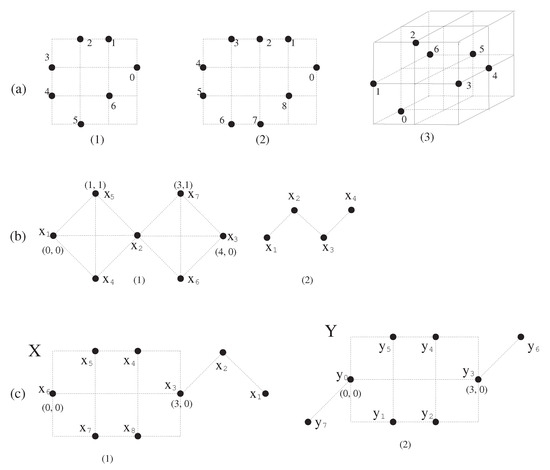
(Case 1) In the case $k:=k(1,n)=2n$, according to the notion of $C_k^{n,l}$, it is clear that the number l should be an even number $l\in {\mathbb{N}}_0\backslash \left\{2\right\}$. For instance, let us consider $C_4^{2,2a}$, $a\in \mathbb{N}\backslash \{1,3\}$ and $C_6^{3,2a}$, $a\in \mathbb{N}\backslash \left\{1\right\}$.

(Case 2) In view of the concept of $C_k^{n,l}(n\in \{2,3\})$, it is obvious that no $C_k^{n,5}$ exists. For instance, neither $C_8^{2,5}$ nor $C_{18}^{3,5}$ exists. However, the existence of $C_k^{n,6}$ depends on both k and n. To be precise, the number $2a$ of $C_{2n}^{n,2a}$ depends on the situation. For instance, while we can take $C_6^{3,6}$, no $C_4^{2,6}$ exists.

(Case 3) In the case $k\ne 2n$, as to $C_k^{n,l}$, if $l\ge 7,n\in \mathbb{N}\backslash \left\{1\right\}$, then it is clear that the number l can be even or odd (see Figure 1a). For instance, consider $C_8^{2,7}$, $C_8^{2,9}$, and $C_{18}^{3,7}$ (see Figure 1a (1)–(3)). In general, $C_k^{n,2a}$ and $C_k^{n,2a+1}$ are considered depending on the dimension $n\in \mathbb{N}\backslash \left\{1\right\}$, and $a\ge 3,a\in \mathbb{N}$. In addition, $C_k^{n,4}$ is admissible. For instance, consider $C_8^{2,4}$, $C_{18}^{3,4}$, $C_{26}^{3,4}$ and so on.

Figure 1. (a) (1) $C_8^{2,7}$ (2) $C_8^{2,9}$ (3) $C_{18}^{3,7}$. (b) (1) $C_8^{2,4}\vee C_8^{2,4}$ [3] (2) A simple 8-path with the length 3, where $x_1=(0,0),x_2=(1,1),x_3=(2,0),x_4=(3,1)$. (c) (1) Digital wedge $X:=C_8^{2,6}\vee P_2$, where $P_2$ is a simple 8-path $\{x_1,x_2,x_3\}$ with the length 2. (2) Digital wedge $Y:=P_1\vee C_8^{2,6}\vee P_1^{\prime }$, where each of $P_1:=\{y_0,y_7\}$ and $P_1^{\prime }:=\{y_3,y_6\}$ is a simple 8-path with the length 1.

Owing to Remark 1, in terms of the number l of $C_k^{n,l}$, the following properties of are observed.

$$\left\{\begin{array}{c}\left(1\right)\mathrm{In}\mathrm{the}\mathrm{case}k=2n(n\notin \{1,2\}),\mathrm{we}\mathrm{obtain}l\in {\mathbb{N}}_0\backslash \left\{2\right\};\hfill \\ \left(2\right)\mathrm{in}\mathrm{the}\mathrm{case}k=4,\mathrm{we}\mathrm{have}l\in {\mathbb{N}}_0\backslash \{2,6\},\mathrm{that}\mathrm{is},\mathrm{neither}{C}_4^{2,5}\mathrm{nor}{C}_4^{2,6}\mathrm{exists};\mathrm{and}\hfill \\ \left(3\right)\mathrm{in}\mathrm{the}\mathrm{case}k\ne 2n(n\in \{2,3\left\}\right),\mathrm{we}\mathrm{obtain}l\in \mathbb{N}\backslash \{1,2,3,5\}.\hfill \\ \mathrm{Namely},\mathrm{none}\mathrm{of}{C}_8^{2,5},C_{18}^{3,5}\mathrm{or}{C}_{26}^{3,5}\mathrm{exists}.\hfill \end{array}\right.$$

(2)

For instance, we can consider $C_4^{2,8}$, $C_8^{2,6}$, $C_8^{2,7}$, $C_8^{2,9}$ and so on. Hereafter, regarding l of $C_k^{n,l}$, we will follow the property (2).

Given $(X,k)$ and a point $x_0\in X$, the following notion of “digital k-neighborhood of $x_0$ with radius 1” is defined, as follows [12]:

$$N_k(x_0,1):=\{x\in X|x\mathrm{is}k-\mathrm{adjacent}\mathrm{to}{x}_0\}\cup \left\{x_0\right\}.$$

(3)

For more general cases of $N_k(x_0,\epsilon ),\epsilon \in \mathbb{N}$, see References [7,12]. The digital $(k_0,k_1)$-continuity of a map $f:(X,k_0)\to (Y,k_1)$ in Reference [11] can be represented by using the k-neighborhood in (3), as follows:

Proposition 1.

[12] A function $f:(X,k_0)\to (Y,k_1)$ is (digitally) $(k_0,k_1)$-continuous if and only if for every $x\in X$, $f\left(N_{k_0}(x,1)\right)\subset N_{k_1}(f\left(x\right),1)$.

In Proposition 1, in the case $k:=k_0=k_1$, the map f is called a ‘k-continuous’ map to abbreviate the $(k,k)$-continuity of the given map f. Using the digital continuity of maps between two digital images, let us recall the category DTC consisting of the following two pieces of data [12], called the digital topological category, as follows:

The set of $(X,k)$, where $X\subset {\mathbb{Z}}^n$, as objects of DTC denoted by $Ob\left(DTC\right)$;

For every ordered pair of objects $(X_i,k_i),i\in \{0,1\}$, the set of all $(k_0,k_1)$-continuous maps between them as morphisms of DTC, denoted by $Mor\left(DTC\right)$.

In DTC, for the case $k:=k_0=k_1$, we will use the notation DTC(k).

In some literature, since there is a certain confusion of characterizing both a k-path and a $(2,k)$-continuous map, we need to confirm some difference between them, as follows:

Remark 2.

Given a k-path ${\left(x_i\right)}_{i\in M}$ on $(X,k)$, we may establish a $(2,k)$-continuous map $f:{[0,m]}_{\mathbb{Z}}\to (X,k)$ whose image of ${[0,m]}_{\mathbb{Z}}$ by f is considered to be the given k-path, that is, ${\left(f\left(i\right)\right)}_{i\in {[0,m]}_{\mathbb{Z}}}={\left(x_i\right)}_{i\in M}$ as a sequence with $f\left(i\right)=x_i$. However, given a $(2,k)$-continuous map $f:{[0,m]}_{\mathbb{Z}}\to (X,k)$, not every image by the given map f as a sequence, that is, the sequence $\left(f\right(0),f(1),\cdots ,f(m\left)\right)\subset X$, is always a k-path on $(X,k)$ (see the notion of k-path in the previous part) because some of the points $f\left(i\right)$ and $f(i+1)$ can be equal. Of course, depending on the situation, based on this sequence $\left(f\right(0),f(1),\cdots ,f(m\left)\right)\subset X$, we can take a k-path as a subsequence ${\left(x_i\right)}_{i\in M^{\prime }\subset {[0,m]}_{\mathbb{Z}}}$ of $\left(f\right(0),f(1),\cdots ,f(m\left)\right)$.

To compare digital images $(X,k)$ up to similarity, we often use the notion of a $(k_0,k_1)$-isomorphism (or k-isomorphism), as follows:

Definition 1.

[8] ($(k_0,k_1)$-homeomorphism in Reference [17]) Consider two digital images $(Z,k_0)$ and $(W,k_1)$ in ${\mathbb{Z}}^{n_0}$ and ${\mathbb{Z}}^{n_1}$, respectively. Then, a map $h:Z\to W$ is called a $(k_0,k_1)$-isomorphism if h is a $(k_0,k_1)$-continuous bijection and further, $h^{-1}:W\to Z$ is $(k_1,k_0)$-continuous. Then, we use the notation $Z{\approx }_{(k_0,k_1)}W$. In the case $k:=k_0=k_1$, the map h is called a k-isomorphism.

Let us now recall the notions of a digital wedge which can be used in studying fixed point sets from the viewpoint of digital geometry. Given two digital images $(A,k)$ and $(B,k)$, a digital wedge, denoted by $(A\vee B,k)$, is initially defined [8,12] as the union of the digital images $(A^{\prime },k)$ and $(B^{\prime },k)$ (for more details see Figure 1, Figure 2, Figure 3 and Figure 4), where

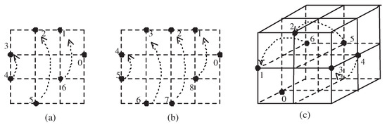
Figure 2. Configuration of $F\left(Co{n}_8\left(C_8^{n,l}\right)\right)$ for the particular cases given in Example 1, where l is odd. (a) Regarding $F\left(Co{n}_8\left(C_8^{2,7}\right)\right)$, we observe $Im{\left(f\right)}^{♯}=4$. (b) Concerning $F\left(Co{n}_8\left(C_8^{2,9}\right)\right)$, we see $Im{\left(f\right)}^{♯}=5$. (c) Regarding $F\left(Co{n}_{18}\left(C_{18}^{3,7}\right)\right)$, we find $Im{\left(f\right)}^{♯}=4$.

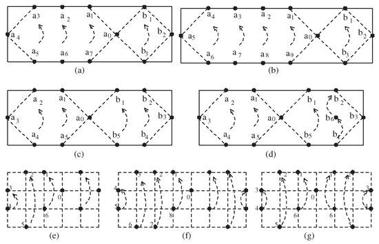
Figure 3. (a) $C_8^{2,8}\vee C_8^{2,4}$ [3] whose digital 8-fundamental group is isomorphic to $(\mathbb{Z},+)$ and $F\left(Co{n}_8(C_8^{2,8}\vee C_8^{2,4})\right)$ is perfect. (b) $C_8^{2,10}\vee C_8^{2,4}$[3] whose digital 8-fundamental group is isomorphic to $(\mathbb{Z},+)$ and $F\left(Co{n}_8(C_8^{2,10}\vee C_8^{2,4})\right)$ is perfect. (c) $F\left(Co{n}_8(C_8^{2,6}\vee C_8^{2,6})\right)$ is not perfect. (d) Configuration of $F(Co{n}_8(C_8^{2,6}\vee Y)$ is perfect, where $Y:=\{a_0,b_i|i\in {[1,6]}_{\mathbb{Z}}\}$. In particular, while $C_8^{2,6}\vee Y$ is not 8-contractible, $F\left(Co{n}_8(C_8^{2,6}\vee Y)\right)$ is perfect. (e) $F\left(Co{n}_8(C_8^{2,7}\vee C_8^{2,4})\right)$ is perfect. (f) $F\left(Co{n}_8(C_8^{2,9}\vee C_8^{2,7})\right)$ is not perfect. (g) $F\left(Co{n}_8(C_8^{2,7}\vee C_8^{2,7})\right)$ is not perfect.

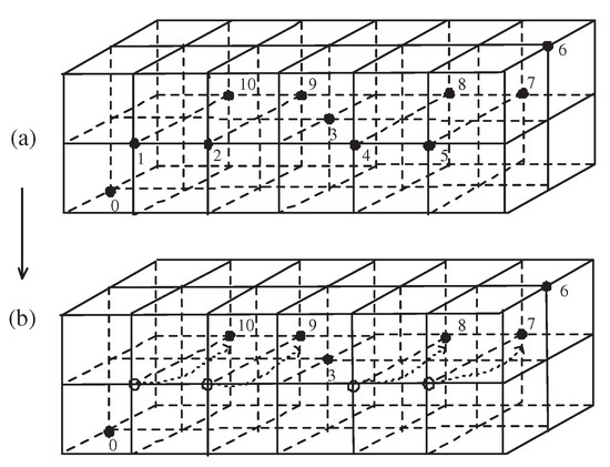
Figure 4. Explanation of the process of obtaining the numbers $m\in {[1,7]}_{\mathbb{Z}}\subset F\left(Co{n}_{26}(C_{26}^{3,6}\vee C_{26}^{3,6})\right)$ (see (20)–(26). Establishment of a simple 26-path from the given digital wedge $C_{26}^{3,6}\vee C_{26}^{3,6}$ (see $\left(a\right)\to \left(b\right))$.

(1)

$A^{\prime }\cap B^{\prime }$ is a singleton, say $\left\{p\right\}$.

(2)

$A^{\prime }\backslash \left\{p\right\}$ and $B^{\prime }\backslash \left\{p\right\}$ are not k-adjacent, where two sets $(C,k)$ and $(D,k)$ are said to be k-adjacent if $C\cap D=\varnothing$ and there are at least two points $a\in C$ and $b\in D$ such that a is k-adjacent to b [14].

(3)

$(A^{\prime },k)$ is k-isomorphic to $(A,k)$ and $(B^{\prime },k)$ is k-isomorphic to $(B,k)$ (see Definition 1).

When studying digital wedges in a $DTC\left(k\right)$ setting, we are strongly required to follow this approach. Besides, $A\vee B$ might be considered to be $A^{\prime }\vee B^{\prime }$. Indeed, this digital wedge is quite different from the classical one point union (or wedge) in typical topology [18] and standard graph theory [19] by the k-adjacency referred to in (2) above.

A digital topological version of the strong graph adjacency of a product of two typical graphs [20] was initially developed in Reference [12]. It is called a normal adjacency of digital product [8]. Indeed, this notion is strongly related to the calculation of digital fundamental groups of digital products [9] and further, an automorphism group of a digital covering space of a digital product [9] (see Theorem 2 and Corollary 1 below).

Motivated by the pointed digital k-homotopy in References [21,22] (see also Reference [17]), the concept of k-homotopy relative to a subset $A\subset X$ is established, as follows:

Definition 2.

[12,17] Let $((X,A),k_0)$ and $(Y,k_1)$ be a digital image pair and a digital image in ${\mathbb{Z}}^{n_0}$ and ${\mathbb{Z}}^{n_1}$, respectively. Let $f,g:X\to Y$ be $(k_0,k_1)$-continuous functions. Suppose there exist $m\in \mathbb{N}$ and a function $H:X\times {[0,m]}_{\mathbb{Z}}\to Y$ such that

(1) 

for all $x\in X,H(x,0)=f\left(x\right)$ and $H(x,m)=g\left(x\right)$;

(2) 

for all $t\in {[0,m]}_{\mathbb{Z}}$, the induced function $H_t:X\to Y$ given by $H_t\left(x\right)=H(x,t)$ for all $x\in X$ is $(k_0,k_1)$-continuous.

(3) 

for all $x\in X$, the induced function $H_x:{[0,m]}_{\mathbb{Z}}\to Y$ given by

$H_x\left(t\right)=H(x,t)$ for all $t\in {[0,m]}_{\mathbb{Z}}$ is $(2,k_1)$-continuous; Then, H is said to be a $(k_0,k_1)$-homotopy between f and g [17].

(4) 

Furthermore, for all $t\in {[0,m]}_{\mathbb{Z}}$, $H_t\left(x\right)=f\left(x\right)=g\left(x\right)$ for all $x\in A$ and for all $t\in {[0,m]}_{\mathbb{Z}}$ [12].

Then, we call H a $(k_0,k_1)$-homotopy relative to A between f and g, and f and g are said to be $(k_0,k_1)$-homotopic relative to A in Y, $f{\simeq }_{(k_0,k_1)rel.A}g$ in symbols [12].

In Definition 2, if $A=\left\{x_0\right\}\subset X$, then we say that F is a pointed $(k_0,k_1)$-homotopy at $\left\{x_0\right\}$ [17]. In the case $k:=k_0=k_1$ and $n_0=n_1$, we call a k-homotopy to abbreviate $(k_0,k_1)$-homotopy. If, for some $x_0\in X$, $1_X$ is k-homotopic to the constant map in the space X relative to $\left\{x_0\right\}$, then $(X,x_0)$ is said to be pointed k-contractible [17].

Based on this k-homotopy, the notion of digital homotopy equivalence firstly introduced in Reference [23], as follows:

Definition 3.

[23] Given two digital images $(Z,k)$ and $(W,k)$, if there are k-continuous maps $h:Z\to W$ and $l:W\to Z$ such that the composite $l\circ h$ is k-homotopic to $1_Z$ and the composite $h\circ l$ is k-homotopic to $1_W$, then the map $h:Z\to W$ is called a k-homotopy equivalence and is denoted by $Z{\simeq }_{k·h·e}W$. Besides, $(Z,k)$ is said to be k-homotopy equivalent to $(W,k)$. If the identity map $1_Z$ is k-homotopy equivalent to a certain constant map $c_{\left\{z_0\right\}},z_0\in Z$, we say that $(Z,k)$ is k-contractible. In particular, in the case $(Z,k_0)$ and $(W,k_1)$, the map h is called a $(k_0,k_1)$-homotopy equivalence.

With the several concepts such as digital k-homotopy class [21,22], Khalimsky operation of two k-homotopy classes [21], trivial extension [17], Reference [17] defined the digital k-fundamental group, denoted by ${\pi }^k(X,x_0),x_0\in X$. Also, we have the following: If X is pointed k-contractible, then it is clear that ${\pi }^k(X,x_0)$ is a trivial group [17]. Using the homotopy lifting theorem, and the unique digital lifting theorem [12], we obtain the following [12]:

Theorem 1.

[12] (1) For a non-k-contractible $C_k^{n,l}$, ${\pi }^k\left(C_k^{n,l}\right)$ is an infinite cyclic group.

(2) For two non-k-contractible spaces $C_k^{n,l_i},i\in \{1,2\}$, ${\pi }^k(C_k^{n,l_1}\vee C_k^{n,l_2})$ is a free group with two generators of which they have infinite orders.

For instance, ${\pi }^8(C_8^{2,6}\vee C_8^{2,8})$ is a free group with two generators, $\mathbb{Z}\ast \mathbb{Z}$.

Given two digital images $(X_i,k_i)$ in ${\mathbb{Z}}^{n_i},i\in \{1,2\}$, consider the digital product $X_1\times X_2$ in ${\mathbb{Z}}^{n_1+n_2}$. For every point $p:=(x,y)\in X_1\times X_2$, if there is a k-adjacency of ${\mathbb{Z}}^{n_1+n_2}$ (see (1)) such that $N_k(p,1)=N_{k_1}(x,1)\times \left\{y\right\}\cup \left\{x\right\}\times N_{k_2}(y,1)$, then we say that the k-adjacency for $X_1\times X_2$ is C-compatible [9]. Since both the k-fundamental group and the k-contractibility of a digital image $(X,k)$ are so related to the study of $F\left(Co{n}_k\left(X\right)\right))$ (see Theorem 4), we need to recall the following properties.

Theorem 2.

[9] Assume that $C_{k_i}^{n_i,l_i}$ is a simple closed $k_i$-curve with $l_i$ elements in ${\mathbb{Z}}^i,i\in \{1,2\}$, and they are not $k_i$-contractible. If there is a C-compatible k-adjacency of its digital product $C_{k_1}^{n_1,l_1}\times C_{k_2}^{n_2,l_2}$, then the k-fundamental group ${\pi }^k(C_{k_1}^{n_1,l_1}\times C_{k_2}^{n_2,l_2})$ is isomorphic to ${\pi }^k\left(C_{k_1}^{n_1,l_1}\right)\times {\pi }^k\left(C_{k_2}^{n_2,l_2}\right)$.

Theorem 2 strongly facilitates the classification of digital covering spaces [12], as follows:

Corollary 1.

[9] Assume a digital product $C_{k_1}^{n_1,l_1}\times C_{k_2}^{n_2,l_2}$ with a C-compatible k-adjacency. Let $(\mathbb{Z},p_i,C_{k_i}^{n_i,l_i})$ be a radius 2-$(2,k_i)$-covering map, $i\in \{1,2\}$, where $C_{k_i}^{n_i,l_i}:={\left(x_i\right)}_{i\in {[0,l_i-1]}_{\mathbb{Z}}}$ and $p_i\left(t\right)=x_{t\left(mod{l}_i\right)}$. Then, the automorphism group $Aut(\mathbb{Z}\times \mathbb{Z}|C_{k_1}^{n_1,l_1}\times C_{k_2}^{n_2,l_2})$ is isomorphic to the group $(l_1\mathbb{Z}\times l_2\mathbb{Z},+)$.

3. Existence of a Perfect Alignment of Fixed Point Sets

This section explores some conditions that make an alignment of fixed point sets of a digital image 2-connected (or perfect). As usual, we say that a digital topological property is a property of a digital image $(X,k)$ which is invariant under digital k-isomorphisms. As mentioned in the previous part, this paper takes the notation $F\left(Co{n}_k\left(X\right)\right)$ to highlight the set of k-continuous self-maps of $(X,k)$, as follows:

$$F\left(Co{n}_k\left(X\right)\right):=\left\{Fix{\left(f\right)}^{♯}\right|f\mathrm{is}\mathrm{a}k-\mathrm{continuous}\mathrm{self}-\mathrm{map}\mathrm{of}X\},$$

(4)

where $Fix\left(f\right):=\{x\in X|f\left(x\right)=x\}.$ Using the set in (4), we define the following:

Definition 4.

[3] Given $(X,k)$, $F\left(Co{n}_k\left(X\right)\right):=(F\left(Co{n}_k\left(X\right)\right),2)$ is said to be an alignment of fixed point sets of $(X,k)$.

A paper [2] only used the notation $F\left(X\right):=F\left(Co{n}_k\left(X\right)\right)$ as just a set without the 2-adjacency. In Definition 4, we remind that the pair $(F\left(Co{n}_k\left(X\right)\right),2)$ is assumed to be a digital image with 2-adjacency as a subset of $(\mathbb{Z},2)$.

Definition 5.

[3] Given $(X,k)$, if $F\left(Co{n}_k\left(X\right)\right)={[0,X^{♯}]}_{\mathbb{Z}}$, then $(F\left(Co{n}_k\left(X\right)\right),2)$ (or $F\left(Co{n}_k\left(X\right)\right)$ for brevity) is said to be perfect.

This notion can play an important role in studying motions of rigid objects with fixed points in the field of robotics.

Theorem 3.

In $DTC\left(k\right)$, $F\left(Co{n}_k\left(X\right)\right)$ is a digital topological property [2,3].

Proof. 

For two k-isomorphic images $(X,k)$ and $(Y,k)$, since we have $F\left(Co{n}_k\left(X\right)\right)=F\left(Co{n}_k\left(Y\right)\right)$ (see Corollary 4.4 of Reference [2]), the proof is completed.  ☐

Given $C_k^{n,l}$, we obviously obtain the following:

Lemma 1.

(1) $F\left(Co{n}_4\left(C_4^{2,4}\right)\right)={[0,4]}_{\mathbb{Z}}$ [2,3].

(2) $F\left(Co{n}_{3^n-1}\left(C_{3^n-1}^{n,4}\right)\right)={[0,4]}_{\mathbb{Z}}$ [3].

(3) For $l\in {\mathbb{N}}_0$, $F\left(Co{n}_k\left(C_k^{n,l}\right)\right)={[0,\frac{l}{2}+1]}_{\mathbb{Z}}\cup \left\{l\right\}$ [2].

(4) In the case $l\in {\mathbb{N}}_0\backslash \left\{2\right\}$, $F{\left(Co{n}_k\left(C_k^{n,l}\right)\right)}^{♯}=\frac{l+6}{2}$.

References [2,3] (or arXiv version of [2]) studied $F\left(Co{n}_k\left(C_k^{n,l}\right)\right)$ only for the case of even number l (see Lemma 1). After recalling Remark 1, let us now formulate $F\left(Co{n}_k\left(C_k^{n,l}\right)\right)$ for an odd number l of $C_k^{n,l},k\ne 2n$.

Lemma 2.

For an odd number l of $C_k^{n,l},k\ne 2n$, $F\left(Co{n}_k\left(C_k^{n,l}\right)\right)={[0,\frac{l+1}{2}]}_{\mathbb{Z}}\cup \left\{l\right\}$, that is, $F{\left(Co{n}_k\left(C_k^{n,l}\right)\right)}^{♯}=\frac{l+5}{2}$.

Proof. 

Regarding the assertion, it is clear that

$$0,1,l\in F\left(Co{n}_k\left(C_k^{n,l}\right)\right),$$

(5)

because only a singleton digital image has the fixed point property [11,24] (for more details see Remark 10 of [7]), a constant map is also a k-continuous map, and the identity map of $(X,k)$ is obviously a k-continuous self-map of $(X,k)$. Thus, it suffices to consider certain k-continuous self-maps f of $C_k^{n,l}$ such that $f\left(C_k^{n,l}\right)⊊C_k^{n,l}$, that is, $f{\left(C_k^{n,l}\right)}^{♯}\le l-1$. Then, this set $f\left(C_k^{n,l}\right)$ should be a certain k-path which is not a simple k-cycle (or a certain simple closed k-curve) on $C_k^{n,l}:={\left(x_i\right)}_{i\in {[0,l-1]}_{\mathbb{Z}}}$. More precisely, consider the map (see Figure 2)

$$f:C_k^{n,l}\to C_k^{n,l}$$

defined by

$$\left\{\begin{array}{c}f\left(x_{l-i}\right)=x_i,i\in {[1,\frac{l-1}{2}]}_{\mathbb{Z}},\mathrm{and}\hfill \\ f\left(x\right)=x,x\in C_k^{n,l}\backslash \{x_{\frac{l+1}{2}},\cdots ,x_{l-1}\}=\left\{x_i\right|i\in {[0,\frac{l-1}{2}]}_{\mathbb{Z}}\}.\hfill \end{array}\right.$$

(6)

Then, this map f is a k-continuous self-map of $C_k^{n,l}$ such that $Fix{\left(f\right)}^{♯}=\frac{l+1}{2}$ (see (6) with Proposition 1), where $Fix\left(f\right):=\{x\in C_k^{n,l}|f\left(x\right)=x\}$. In view of Proposition 1, the image by the map $f(\ne 1_{C_k^{n,l}})$ proposed in (6) has the maximal number of the set (for instance, see Figure 2a–c)

$$\left\{Fix{\left(f\right)}^{♯}\right|f(\ne 1_{C_k^{n,l}})\mathrm{is}\mathrm{a}k-\mathrm{continuous}\mathrm{self}-\mathrm{map}\mathrm{of}{C}_k^{n,l}\}.$$

Namely, we obtain

$$\frac{l+1}{2}=\max \left\{Fix{\left(f\right)}^{♯}\right|f(\ne 1_{C_k^{n,l}})\mathrm{is}\mathrm{a}k-\mathrm{continuous}\mathrm{self}-\mathrm{map}\mathrm{of}{C}_k^{n,l}\}.$$

(7)

Indeed, for each number $m⪇\frac{l+1}{2}$, it is clear that there are many types of k-continuous self-maps g of $C_k^{n,l}$ depending on the number l such that

$$Fix{\left(g\right)}^{♯}=m(\mathrm{see}\mathrm{the}k-\mathrm{connected}\mathrm{subset}\mathrm{of}Im\left(f\right)\mathrm{in}\mathrm{Figure}2,k\in \{8,18\}).$$

(8)

By (5), (7), and (8), we conclude that $F\left(Co{n}_k\left(C_k^{n,l}\right)\right)={[0,\frac{l+1}{2}]}_{\mathbb{Z}}\cup \left\{l\right\}$.  ☐

Example 1.

(1) $F\left(Co{n}_8\left(C_8^{2,7}\right)\right)={[0,4]}_{\mathbb{Z}}\cup \left\{7\right\}$. To be precise, for convenience, let us consider the self-map f of $C_8^{2,7}:={\left(x_i\right)}_{i\in {[0,6]}_{\mathbb{Z}}}$ in Figure 2a with $i:=x_i$. Then, regarding $F\left(Co{n}_8\left(C_8^{2,7}\right)\right)$, according to the map in (6), consider the map

$$f:C_8^{2,7}\to C_8^{2,7}\mathit{defined}\mathit{by}$$

$$\left\{\begin{array}{cc}\hfill & f\left(x_6\right)=x_1,f\left(x_5\right)=x_2,f\left(x_4\right)=x_3,\mathit{and}\hfill \\ \hfill & f\left(x\right)=x,x\in C_8^{2,7}\backslash \{x_4,x_5,x_6\}.\hfill \end{array}\right.$$

Then, it is clear that f is an 8-continuous map with $Fix{\left(f\right)}^{♯}=4$. Similarly, for any $m\in {[1,3]}_{\mathbb{Z}}$, we can have another several 8-continuous self-maps g of $C_8^{2,7}$ such that $Fix{\left(g\right)}^{♯}=m$. Hence we have $F\left(Co{n}_8\left(C_8^{2,7}\right)\right)={[0,4]}_{\mathbb{Z}}\cup \left\{7\right\}$ because it is clear that $0,7\in F\left(Co{n}_8\left(C_8^{2,7}\right)\right)$.

Similarly, we obtain the following:

(2)

$F\left(Co{n}_8\left(C_8^{2,9}\right)\right)={[0,5]}_{\mathbb{Z}}\cup \left\{9\right\}$ (see Figure 2b).

(3)

$F\left(Co{n}_{18}\left(C_{18}^{3,7}\right)\right)={[0,4]}_{\mathbb{Z}}\cup \left\{7\right\}$ (see Figure 2c).

For a digital image $(X,k)$ which is k-connected and $X^{♯}\ge 2$, it is clear that $\{0,1,X^{♯}\}\subset F\left(Co{n}_k\left(X\right)\right)$[2] and further, by Lemmas 1 and 2, and the property (2), we obtain the following: For any l of $C_k^{n,l}$ and $m_i$ of $C_k^{n,m_i},i\in \{1,2\}$,

$$\left\{\begin{array}{c}\left(1\right)5\le F{\left(Co{n}_k\left(C_k^{n,l}\right)\right)}^{♯}\le l+1\mathrm{and}\hfill \\ \left(2\right)\mathrm{if}{m}_1\le m_2,\mathrm{we}\mathrm{obtain}F\left(Co{n}_k\left(C_k^{n,m_1}\right)\right)\subset F\left(Co{n}_k\left(C_k^{n,m_2}\right)\right).\hfill \end{array}\right.$$

(9)

In (9)(2), the set $C_k^{n,m_1}$ need not be a subset of $C_k^{n,m_2}$. For instance, $F{\left(Co{n}_8\left(C_8^{2,4}\right)\right)}^{♯}=5$ and $F{\left(Co{n}_8\left(C_8^{2,7}\right)\right)}^{♯}=6$. Besides, using Lemma 1(3) and Lemma 2, we observe $F\left(Co{n}_8\left(C_8^{2,6}\right)\right)={[0,4]}_{\mathbb{Z}}\cup \left\{6\right\}=F\left(Co{n}_8\left(C_8^{2,7}\right)\right)$.

Given $(X,k)$ with $X^{♯}=n$, we need to check if there is the number $n-1\in F\left(Co{n}_k\left(X\right)\right)$. Indeed, a paper [2] studied this property with the following lemma (see Lemma 4.8 of Reference [2]).

Lemma 3.

[2] Let X be connected with $n=X^{♯}$. Then, $n-1\in F\left(X\right)$ if and only if there are distinct points $x_1,x_2\in X$ with $N\left(x_1\right)\subset N^{\ast }\left(x_2\right)$.

Unlike the notations $N\left(x_1\right)$ and $N^{\ast }\left(x_2\right)$ in Lemma 3, in digital topology we have ordinarily used the following notations: For a given digital image $(X,k)\subset ({\mathbb{Z}}^n,k),n\in \mathbb{N}$, using the digital k-connectivity of (1), we are used to take the following notations [11,12,14]. According to the literature, for $p\in X\subset {\mathbb{Z}}^n$, we recall the notations [11,12,14]

(1)

$N_k\left(p\right):=\{x\in {\mathbb{Z}}^n|x\mathrm{is}k-\mathrm{adjacent}\mathrm{to}p\}\subset {\mathbb{Z}}^n$;

(2)

$N_k^{*}\left(p\right):=N_k\left(p\right)\cup \left\{p\right\}\subset {\mathbb{Z}}^n$;

(3)

$N_k(p,1):=N_k^{*}\left(p\right)\cap X$ (see the notation in (3)); and

(4)

We may represent $N_k(p,1)$ of (3) above in such a way that

$N_k(p,1):=\{x\in X|x\mathrm{is}k-\mathrm{adjacent}\mathrm{to}p\}\cup \left\{p\right\}$, that is, the notation of $N_k(p,1)$ of (3).

The notations $N\left(x_1\right)$ and $N^{*}\left(x_2\right)$ in Lemma 3 are defined, as follows:

$$N\left(x_1\right):=N_k(x_1,1)\backslash \left\{x_1\right\}\mathrm{and}{N}^{*}\left(x_2\right):=N_k(x_2,1).$$

(10)

A recent paper [3] contains some incorrect part in Remark 3 of Reference [3]. Indeed, the remark was based on the preprint posted in arXiv “Fixed point sets in Digital topology, 1(2019), 1-25” which is the preprint version of Reference [2]. Then, there was not any introduction of $N_k\left(x\right)$ and $N_k^{*}\left(x\right)$ in this preprint. With the notion in (10), the current version of Lemma 3 above is correct anyway (disregard the lines 4–11 from the bottom of the page 11 of Reference [3]). But, owing to the unusual notations of $N_k^{*}\left(p\right)$ and $N_k\left(p\right)$ in Lemma 3, a reader can invoke some confusion. Thus, after following the standard notations referred to in (1)–(4) above, we can avoid some potential confusion. Thus, we had better follow the popular and standard notations as stated in (1)–(4) above to finally obtain the following representation of Lemma 3.

Lemma 4

(Representation of Lemma 3). Let $(X,k)$ be k-connected with $n=X^{♯}$. Then, $n-1\in F\left(Co{n}_k\left(X\right)\right)$ if and only if there are distinct points $x_1,x_2\in X$ with $N_k(x_1,1)\backslash \left\{x_1\right\}\subset N_k(x_2,1)$.

Remark 3.

Unlike Lemma 1(3), using Lemma 2, we can deal with $F\left(Co{n}_k(C_k^{n,2a+1}\vee C_k^{n,4})\right)$, $a\in \mathbb{N}\backslash \{1,2\},k\ne 2n$. For insance, we obtain $F\left(Co{n}_8(C_8^{2,7}\vee C_8^{2,4})\right)={[0,10]}_{\mathbb{Z}}$.

Since the notion of k-retract also play an important role in studying $F\left(Co{n}_k\left(X\right)\right)$, let us now recall it, as follows: For $A\subset X$, we say that $(A,k)$ is a k-retract of $(X,k)$ [17] if there is a k-continuous map $r:(X,k)\to (A,k)$ such that for any $a\in A$, $r\left(a\right)=a$. Then, we call the map r a k-retraction from $(X,k)$ onto $(A,k)$.

As mentioned in Section 2, the notion of k-contractibility of $(X,k)$ strongly contributes to the study of $F\left(Co{n}_k\left(X\right)\right)$. Indeed, the following 6-contractibility of the given digital image in Lemma 5 has been often used in digital topology [7,24]. To be precise, given a digital image $(X,k)$ with $X^{♯}=n$, in order to examine if $n-1$ belongs to $F\left(Co{n}_k\left(X\right)\right)$, Reference [2] has used the following property.

Lemma 5.

[7,24] Let $(X:=({[0,1]}_{\mathbb{Z}}^3,6)$ be the digital unit cube with 6-adjacency. Then, it is 6-contractible.

To be specific, though $(X:={[0,1]}_{\mathbb{Z}}^3,6)$ is 6-contractible, it is clear that $7\notin F\left(Co{n}_6\left(X\right)\right)$ [2]. However, we need to point out that the 6-contractibility of this 3-dimensional digital cube $(X,6)$ was already proven in References [7,24] (see Theorem 2.6(1) of Reference [24] and Remark 2(2) of Reference [7]).

Since each of $C_k^{n,l}$, $C_k^{n,l_1}\vee C_k^{n,l_2}$, $\stackrel{\mathrm{m}-\mathrm{times}}{\overbrace{C_k^{n,l}\vee \cdots \vee C_k^{n,l}}}$, and $\stackrel{\mathrm{m}-\mathrm{times}}{\overbrace{C_k^{n,l}\vee \cdots \vee C_k^{n,l}}}\vee \stackrel{\mathrm{t}-\mathrm{times}}{\overbrace{C_k^{n,4}\vee \cdots \vee C_k^{n,4}}},m\in \mathbb{N}$, plays an important role in digital topology (see Theorem 1), let us intensively explore alignments of the fixed point sets of them, for example,

$$\left\{\begin{array}{c}F\left(Co{n}_k\left(C_k^{n,l}\right)\right),\hfill \\ F\left(Co{n}_k(C_k^{n,l_1}\vee C_k^{n,l_2})\right),\hfill \\ F\left(Co{n}_k\left(\stackrel{\mathrm{m}-\mathrm{times}}{\overbrace{C_k^{n,l}\vee \cdots \vee C_k^{n,l}}}\right)\right),\mathrm{and}\hfill \\ F\left(Co{n}_k(\stackrel{\mathrm{m}-\mathrm{times}}{\overbrace{C_k^{n,l}\vee \cdots \vee C_k^{n,l}}}\vee \stackrel{\mathrm{t}-\mathrm{times}}{\overbrace{C_k^{n,4}\vee \cdots \vee C_k^{n,4}}})\right).\hfill \end{array}\right.$$

As a representation of Lemma 1 of Reference [3], for any l of $C_k^{n,l}$ we obtain the following (see Remark 1):

Theorem 4.

$F\left(Co{n}_k\left(C_k^{n,l}\right)\right)$ is perfect if and only if ${\pi }^k\left(C_k^{n,l}\right)$ is trivial.

Proof. 

Using “Contrapositive law”, let us suppose that ${\pi }^k\left(C_k^{n,l}\right)$ is not trivial. Then, by Theorem 1, it is obvious that $C_k^{n,l}$ is not k-contractible. Namely, by Remark 1, we obtain at least $l\ge 6$. In this case, by Lemmas 1(3) and 2, we need to consider the following two cases:

(Case 1) In the case l is even, by Lemma 1(3), we obtain $F\left(Co{n}_k\left(C_k^{n,l}\right)\right)={[0,\frac{l}{2}+1]}_{\mathbb{Z}}\cup \left\{l\right\}$. Hence, if $l\ge 6$, then $F\left(Co{n}_k\left(C_k^{n,l}\right)\right)$ is not perfect because $l-(\frac{l}{2}+1)=\frac{l}{2}-1\ge 2$ (see the difference between $\frac{l}{2}+1$ and l in Lemma 1(3)).

(Case 2) In the case l is odd, by Lemma 2, we have $F\left(Co{n}_k\left(C_k^{n,l}\right)\right)={[0,\frac{l+1}{2}]}_{\mathbb{Z}}\cup \left\{l\right\}$. Hence, if $l\ge 7$, then $F\left(Co{n}_k\left(C_k^{n,l}\right)\right)$ is not perfect because $l-\frac{l+1}{2}=\frac{l-1}{2}\ge 2$ (see the difference between $\frac{l+1}{2}$ and l).

Conversely, if ${\pi }^k\left(C_k^{n,l}\right)$ is trivial, by Theorem 1, we obtain $l=4$. For instance, we can see the cases $C_4^{2,4}$, $C_{18}^{3,4}$, and $C_{3^n-1}^{n,4}$. Thus, by Theorem 1 and Lemma 1, we clearly obtain $F\left(Co{n}_k\left(C_k^{n,4}\right)\right)={[0,4]}_{\mathbb{Z}}$ which is perfect.  ☐

By Theorem 4, it is clear that $F\left(Co{n}_k\left(C_k^{n,l}\right)\right)$ is perfect if and only if $l=4$. Using Lemmas 3 and 4, we obtain the following result which can play an important role in investigating the perfectness of $F\left(Co{n}_k\left(X\right)\right)$.

Lemma 6.

Given $(X,k)$ which is k-connected, assume that there are two distinct points $x_1,x_2\in X$ such that $N_k(x_1,1)\backslash \left\{x_1\right\}\subset N_k(x_2,1)$. Then, we obtain the following:

(1)

$X\backslash \left\{x_1\right\}$ is k-connected.

(2)

$(X\backslash \left\{x_1\right\},k)$ is a k-retract of $(X,k)$.

Proof. 

In the case $X^{♯}=2$, the proof is straightforward because a singleton $X\backslash \left\{x_1\right\}$ is k-connected (for more details see the notion of k-disconnectedness of Reference [7]). Thus, we may assume $X^{♯}\ge 3$.

(1) With the hypothesis “$N_k(x_1,1)\backslash \left\{x_1\right\}\subset N_k(x_2,1)$”, using “Reductio ad Absurdum”, let us suppose that $X\backslash \left\{x_1\right\}$ is not k-connected. Then, there are non-empty sets $X_1,X_2\subset X\backslash \left\{x_1\right\}$ (for details see the notion of k-disconnectedness in Reference [7]) such that

$$\left\{\begin{array}{c}\left(1\right)X\backslash \left\{x_1\right\}=X_1\cup X_2,X_1\cap X_2=\varnothing ,\mathrm{and}\mathrm{further},\hfill \\ \left(2\right)\mathrm{there}\mathrm{are}\mathrm{not}\mathrm{points}{x}_1^{\prime }\in X_1\mathrm{and}{x}_2^{\prime }\in X_2\mathrm{such}\mathrm{that}\mathrm{they}\mathrm{are}k-\mathrm{adjacent}.\hfill \end{array}\right.$$

(11)

Then, there are at least two points $y_1\in X_1,y_2\in X_2$ such that $y_1,y_2\in N_k(x_1,1)\backslash \left\{x_1\right\}$ because $(X,k)$ is k-connected. Owing to the hypothesis “$N_k(x_1,1)\backslash \left\{x_1\right\}\subset N_k(x_2,1)$”, each $y_1$ and $y_2$ should be in $N_k(x_2,1)$. Then, owing to the condition (11), we have a contradiction.

For instance, see the cases in Figure 1b(1)–(2). To be specific, see the two points $x_1$ and $x_2$ in Figure 1b(1) and the two points $x_1$ and $x_3$ in Figure 1b(2) which support this assertion.

(2) With the hypothesis, let us consider the map

$$r:(X,k)\to (X\backslash \left\{x_1\right\},k)$$

defined by

$$\left\{\begin{array}{c}r\left(x_1\right)=x_2,\mathrm{and}\hfill \\ r\left(x\right)=x,x\in X\backslash \left\{x_1\right\}.\hfill \end{array}\right\}$$

(12)

Then, by Proposition 1, with the hypothesis of this theorem we obtain

$$r\left(N_k(x_1,1)\right)\subset N_k(x_2,1)\mathrm{and}r\left(N_k(x,1)\right)\subset N_k(x,1),x(\ne x_1)\in X.$$

Thus, r is a k-continuous map such that ${r|}_{X\backslash \left\{x_1\right\}}=1_{X\backslash \left\{x_1\right\}}$, where ${r|}_A$ is the restriction of the map r to the given set A. Hence r is a k-retraction from $(X,k)$ onto $(X\backslash \left\{x_1\right\},k)$.  ☐

Lemma 7.

[2] Let $(A,k)$ be a k-retract of $(X,k)$. Then, $F\left(Co{n}_k\left(A\right)\right)\subset F\left(Co{n}_k\left(X\right)\right)$.

When investigating the perfectness of a given digital image, we need the following assertion which answers to the question $\left(Q1\right)$.

Theorem 5.

Let $(X,k)$ be k-connected with $n:=X^{♯}$. If there are three or four distinct points $x_1,x_2,x_3,x_4\in X$ such that $N_k(x_1,1)\backslash \left\{x_1\right\}\subset N_k(x_2,1)$ and further,

$$\left\{\begin{array}{c}\left(1\right)\mathit{the}\mathit{two}\mathit{distinct}\mathit{points}{x}_2,x_3\in X\backslash \left\{x_1\right\}\mathit{has}\mathit{the}\mathit{property},\hfill \\ N_k(x_3,1)\backslash \left\{x_3\right\}\subset N_k(x_2,1)\mathit{or}{N}_k(x_2,1)\backslash \left\{x_2\right\}\subset N_k(x_3,1);\mathit{or}\hfill \\ \left(2\right)\mathit{the}\mathit{two}\mathit{distinct}\mathit{points}{x}_3,x_4\in X\backslash \left\{x_1\right\}\mathit{has}\mathit{the}\mathit{property}\hfill \\ N_k(x_3,1)\backslash \left\{x_3\right\}\subset N_k(x_4,1),\hfill \end{array}\right\}$$

(13)

then, $n-1,n-2\in F\left(Co{n}_k\left(X\right)\right)$.

Proof .

(Case 1) With the hypothesis of (1) of (13), we prove the assertion. By Lemmas 3 and 4, owing to the hypothesis $N_k(x_1,1)\backslash \left\{x_1\right\}\subset N_k(x_2,1)$, it is clear $n-1\in F\left(Co{n}_k\left(X\right)\right)$. Furthermore, in $X_1:=X\backslash \left\{x_1\right\}$, owing to the hypothesis that there are certain two points $x_2,x_3$ in $X_1$ such that

$$N_k(x_3,1)\backslash \left\{x_3\right\}\subset N_k(x_2,1)\mathrm{or}{N}_k(x_2,1)\backslash \left\{x_2\right\}\subset N_k(x_3,1),$$

by Lemmas 4 and 6(1), we obtain $n-2\in F\left(Co{n}_k\left(X_1\right)\right)$ because $X_1^{♯}=n-1$. Owing to the hypothesis $N_k(x_1,1)\backslash \left\{x_1\right\}\subset N_k(x_2,1)$, by Lemma 6(2), we see that $(X_1,k)$ is a k-retract of $(X,k)$. Furthermore, by Lemma 7, we also obtain $n-2\in F\left(Co{n}_k\left(X\right)\right)$ so that both $n-1$ and $n-2$ belong to $F\left(Co{n}_k\left(X\right)\right)$.

For instance, see the cases in Figure 1b(1) and (2) or Figure 1c(1).

(Case 2) With the hypothesis of (2) of (13), we prove the assertion. By Lemmas 3 and 4, owing to the hypothesis $N_k(x_1,1)\backslash \left\{x_1\right\}\subset N_k(x_2,1)$, it is clear that $n-1\in F\left(Co{n}_k\left(X\right)\right)$. Furthermore, in $X_1:=X\backslash \left\{x_1\right\}$, owing to the hypothesis that there are two distinct points $x_3,x_4$ in $X_1$ such that $N_k(x_3,1)\backslash \left\{x_3\right\}\subset N_k(x_4,1)$, by Lemmas 4 and 6, we obtain $n-2\in F\left(Co{n}_k\left(X_1\right)\right)$ because $X_1^{♯}=n-1$. Owing to the condition that $N_k(x_1,1)\backslash \left\{x_1\right\}\subset N_k(x_2,1)$, by Lemma 6(2), we see that $(X_1,k)$ is a k-retract of $(X,k)$. Then, by Lemma 7, we conclude that both $n-1$ and $n-2$ belong to $F\left(Co{n}_k\left(X\right)\right)$. For instance, see the cases in Figure 1b(1) and (2) and Figure 3b(1) and (2).  ☐

Example 2.

(1) For any $l\in {\mathbb{N}}_0\backslash \left\{2\right\}$, we now confirm that (see (8) of Reference [3])

$$F\left(Co{n}_k(C_k^{n,l}\vee C_k^{n,4})\right)={[0,4+\frac{l}{2}]}_{\mathbb{Z}}\cup {[l,l+3]}_{\mathbb{Z}}$$

has at least the elements $l+1,l+2$ because there are at least three points $b_1,b_2,b_3$ in $C_k^{n,4}$ that satisfies the condition (1) of (13) and ${(C_k^{n,l}\vee C_k^{n,4})}^{♯}=l+3.$ For instance, consider the case $X:=C_8^{2,8}\vee C_8^{2,4}$ in Figure 3a. Then, we obtain that $F\left(Co{n}_8(C_8^{2,8}\vee C_8^{2,4})\right)$ has at least the elements $9,10$ because there are at least three points in $C_8^{2,4}\subset C_k^{n,8}\vee C_k^{n,4}$ that satisfies the condition (1) of (13) and ${(C_8^{2,8}\vee C_8^{2,4})}^{♯}=11.$

(2) By Lemmas 2, 3, and 4, since $F\left(Co{n}_8(C_8^{2,9}\vee C_8^{2,7})\right)$ does not have the number 15 (see Figure 3f), we conclude that $F\left(Co{n}_8(C_8^{2,9}\vee C_8^{2,7})\right)$ is not perfect.

(3) By Theorem 5, we obtain $F\left(Co{n}_k\left(\stackrel{t-\mathit{times}}{\overbrace{C_k^{n,4}\vee \cdots \vee C_k^{n,4}}}\right)\right)={[0,3t+1]}_{\mathbb{Z}}$.

Remark 4.

The two conditions (1) and (2) of Theorem 5 are independent.

Proof. 

Let us consider the two digital images $(X,8)$ and $(Y,8)$ with $X^{♯}=8=Y^{♯}$ in Figure 1c. Then, by Lemma 1(3) and Theorem 5, we see that

$$F\left(Co{n}_8\left(X\right)\right)={[0,8]}_{\mathbb{Z}}=F\left(Co{n}_8\left(Y\right)\right).$$

Naively, each $F\left(Co{n}_8\left(X\right)\right)$ and $F\left(Co{n}_8\left(Y\right)\right)$ are perfect so that the numbers $6,7$ belong to $F\left(Co{n}_8\left(X\right)\right)=F\left(Co{n}_8\left(Y\right)\right)$.

For $(X,8)$, since there are the three points $x_1$, $x_2$ and $x_3$ in X such that

$$\left\{\begin{array}{c}{N}_8(x_1,1)\backslash \left\{x_1\right\}\subset N_8(x_2,1)\mathrm{and}\mathrm{further},\hfill \\ x_2,x_3\mathrm{in}X\backslash \left\{x_1\right\}\mathrm{satisfy}\mathrm{the}\mathrm{property}\hfill \\ N_8(x_2,1)\backslash \left\{x_2\right\}\subset N_8(x_3,1).\hfill \end{array}\right.$$

Hence $(X,8)$ satisfies the condition (1) of Theorem 5. However, it is clear that $(X,8)$ does not satisfy the condition (2) of Theorem 5.

Meanwhile, let us now consider the case $(Y,8)$ in Figure 1c(2). Then, there are the following four points $y_0,y_7,y_3,y_6$ in Y such that

$$N_8(y_7,1)\backslash \left\{y_7\right\}\subset N_8(y_0,1)\mathrm{and}{N}_8(y_6,1)\backslash \left\{y_6\right\}\subset N_8(y_3,1).$$

Besides, it is clear that this $(Y,8)$ does not satisfy the condition (1) of Theorem 5.  ☐

Remark 5.

The converse of Theorem 5 does not hold.

Proof. 

Let $Z:=X\backslash \left\{x_1\right\}$ in Figure 1c(1). Naively, consider $Z:=\left\{x_i\right|i\in {[2,8]}_{\mathbb{Z}}\}$ in Figure 1c(1). Then, by Lemmas 1(3) and 4, ${[0,4]}_{\mathbb{Z}}\subset F\left(Co{n}_8\left(Z\right)\right)$ and we also have $5,6,7\in F\left(Co{n}_8\left(Z\right)\right)$ so that it is clear that $F\left(Co{n}_8\left(Z\right)\right)={[0,7]}_{\mathbb{Z}}$ because $Z^{♯}=7$. However, the digital image $(Z,8)$ does not satisfy both of the conditions (1) and (2) of Theorem 5. For instance, in $(Z,8)$, while there are points $x_2,x_3$ such that $N_8(x_2,1)\backslash \left\{x_2\right\}\subset N_8(x_3,1)$, there are no points satisfying either the condition (1) or the condition (2) of (13) in Theorem 5. Namely, $(Z\backslash \left\{x_1\right\},8)$ does not satisfies each of the conditions (1) and (2) of (13).  ☐

Owing to Theorem 5, the following is obtained:

Corollary 2.

Given $(X,k)$ with $X^{♯}=n$, if there is a set $\left\{x_i\right|i\in {[1,l]}_{\mathbb{Z}}\}\subset X$ with $l⪇n$ such that

$$\left\{\begin{array}{c}\left(1\right)N_k(x_1,1)\backslash \left\{x_1\right\}\subset N_k(x_2,1),\hfill \\ \left(2\right)\exists x_3\in X_1:=X\backslash \left\{x_1\right\},\hfill \\ \mathit{such}\mathit{that}{N}_k(x_2,1)\backslash \left\{x_2\right\}\subset N_k(x_3,1)\mathit{in}{X}_1,\hfill \\ \left(3\right)\exists x_4\in X_2:=X\backslash \{x_1,x_2\}\hfill \\ \mathit{such}\mathit{that}{N}_k(x_3,1)\backslash \left\{x_3\right\}\subset N_k\left(x_4\right),1)\mathit{in}{X}_2,\hfill \\ \cdots \hfill \\ \left(l\right)\exists x_l\in X_{l-2}:=X\backslash \{x_1{x}_2,\cdots ,x_{l-2}\},\mathit{and}\hfill \\ \mathit{such}\mathit{that}{N}_k(x_{l-l},1)\backslash \left\{x_{l-1}\right\}\subset N_k(x_l,1)\mathit{in}{X}_{l-2}.\hfill \end{array}\right.$$

(14)

Then, $\{n-1,n-2,\cdots ,n-l+1\}\subset F\left(Co{n}_k\left(X\right)\right)$.

Example 3.

(1) Given a simple k-path $(X,k)$ with $X^{♯}=l$, we obtain $F\left(Co{n}_k\left(X\right)\right)={[0,l]}_{\mathbb{Z}}$.

(2) Let $Y:=\stackrel{\mathit{t}-\mathit{times}}{\overbrace{C_k^{n,4}\vee \cdots \vee C_k^{n,4}}}$. Then, as stated in Example 2(3), $F(Co{n}_k\left(Y\right)={[0,3t+1]}_{\mathbb{Z}}$ which is perfect.

(3) Let $(Z,k)$ be a digital wedge of some simple k-paths. Then, $F\left(Co{n}_k\left(Z\right)\right)$ is perfect.

4. Formulation of $\mathit{F}\left({\mathit{Con}}_{\mathit{k}}\left(\stackrel{\mathbf{m}-\mathbf{times}}{\overbrace{{\mathit{C}}_{\mathit{k}}^{\mathit{n},\mathit{l}}\vee \cdots \vee {\mathit{C}}_{\mathit{k}}^{\mathit{n},\mathit{l}}}}\right)\right),\mathit{l}\in {\mathbb{N}}_{\mathbf{0}}\backslash \left\{\mathbf{2}\right\},\mathit{m}\in \mathbb{N}$

This section initially formulates $F\left(Co{n}_k\left(\stackrel{\mathrm{m}-\mathrm{times}}{\overbrace{C_k^{n,l}\vee \cdots \vee C_k^{n,l}}}\right)\right),m\in \mathbb{N},l\in {\mathbb{N}}_0\backslash \left\{2\right\}$. Then, the following queries are naturally raised (see (Q2) and (Q3)).

(4-1) Under what conditions is $F\left(Co{n}_k\left(\stackrel{\mathrm{m}-\mathrm{times}}{\overbrace{C_k^{n,l}\vee \cdots \vee C_k^{n,l}}}\right)\right)$ perfect ?

(4-2) How many 2-components are there in $F\left(Co{n}_k\left(\stackrel{\mathrm{m}-\mathrm{times}}{\overbrace{C_k^{n,l}\vee \cdots \vee C_k^{n,l}}}\right)\right)$ ?

Since the exploration of the perfectness or non-perfectness of

$F\left(Co{n}_k\left(\stackrel{\mathrm{m}-\mathrm{times}}{\overbrace{C_k^{n,l}\vee \cdots \vee C_k^{n,l}}}\right)\right)$ and $F\left(Co{n}_k(C_k^{n,l}\vee C_k^{n,l}\vee C_k^{n,l}\vee \stackrel{\mathrm{t}-\mathrm{times}}{\overbrace{C_k^{n,4}\vee \cdots \vee C_k^{n,4}}})\right)$ plays an important role in digital geometry, this section intensively studies this topic and its generalization. In particular, we prove that $F\left(Co{n}_k(C_k^{n,l}\vee C_k^{n,l}\vee C_k^{n,l})\right)$ is perfect if and only if $l=4$. Besides, we prove that $F\left(Co{n}_k(C_k^{n,l}\vee C_k^{n,l}\vee C_k^{n,l})\right)$ has two 2-components if and only if $l\ge 6$, as follows:

Theorem 6.

For $l\in {\mathbb{N}}_0$, $F\left(Co{n}_k(C_k^{n,l}\vee C_k^{n,l}\vee C_k^{n,l})\right)={[0,\frac{5l}{2}-1]}_{\mathbb{Z}}\cup \{3l-2\}$.

Proof. 

Though there are many kinds of k-continuous self-maps f of $C_k^{n,l}\vee C_k^{n,l}\vee C_k^{n,l}$, regarding $F\left(Co{n}_k(C_k^{n,l}\vee C_k^{n,l}\vee C_k^{n,l})\right)$, it suffices to consider only the maps f such that

(a)

${f|}_{C_k^{n,l}}\left(x\right)=x$; or

(b)

${f|}_{C_k^{n,l}\vee C_k^{n,l}}\left(x\right)=x$; or

(c)

$f\left(C_k^{n,l}\right)⊊C_k^{n,l}$; or

(d)

f does not have any fixed point of it, where ${f|}_A$ means the restriction function f to the given set A.

Firstly, from (a), since $C_k^{n,l}\vee C_k^{n,l}\vee C_k^{n,l}$ has the cardinality $3l-2$, using Lemma 1(3), we have

$${[l,2l]}_{\mathbb{Z}}\cup \{3l-2\}\subset F\left(Co{n}_k(C_k^{n,l}\vee C_k^{n,l}\vee C_k^{n,l})\right).$$

(15)

Secondly, from (b), using Lemma 1(3), we obtain

$${[2l-1,2l-1+\frac{l}{2}]}_{\mathbb{Z}}\cup \{3l-2\}={[2l-1,\frac{5l}{2}-1]}_{\mathbb{Z}}\cup \{3l-2\}\subset F\left(Co{n}_k(C_k^{n,l}\vee C_k^{n,l}\vee C_k^{n,l})\right).$$

(16)

Thirdly, from (c)–(d), we have

$${[0,\frac{3l}{2}+1]}_{\mathbb{Z}}\subset F\left(Co{n}_k(C_k^{n,l}\vee C_k^{n,l}\vee C_k^{n,l})\right).$$

(17)

After comparing the three numbers $\frac{5l}{2}-1$, $\frac{3l}{2}+1$, and $3l-2$ from (15)–(17), we conclude that

$$F\left(Co{n}_k(C_k^{n,l}\vee C_k^{n,l}\vee C_k^{n,l})\right)={[0,\frac{5l}{2}-1]}_{\mathbb{Z}}\cup \{3l-2\}.$$

(18)

 ☐

By Theorem 6, the following is obtained.

Theorem 7.

(1) For $l\in {\mathbb{N}}_0\backslash \left\{2\right\}$, $F\left(Co{n}_k(C_k^{n,l}\vee C_k^{n,l}\vee C_k^{n,l})\right)$ is perfect if and only if $l=4$.

(2) For $l\in {\mathbb{N}}_0\backslash \left\{2\right\}$, $F\left(Co{n}_k(C_k^{n,l}\vee C_k^{n,l}\vee C_k^{n,l})\right)$ has two 2-components if and only if $l\ge 6$.

Proof. 

(1) Let us now take the difference from (18)

$$(3l-2)-(\frac{5l}{2}-1)=\frac{l}{2}-1$$

(19)

From (19), if $\frac{l}{2}-1\le 1$, then the perfectness of $F\left(Co{n}_k(C_k^{n,l}\vee C_k^{n,l}\vee C_k^{n,l})\right)$ holds. Thus, we obtain the following: $F\left(Co{n}_k(C_k^{n,l}\vee C_k^{n,l}\vee C_k^{n,l})\right)={[0,3l-2]}_{\mathbb{Z}}$ is perfect if and only if $l=4$.

(2) In (19) above, count on the case $\frac{l}{2}-1\ge 2$, that is, $l\ge 6$. In view of (18), we conclude that $F\left(Co{n}_k(C_k^{n,l}\vee C_k^{n,l}\vee C_k^{n,l})\right)$ has the two 2-components ${[0,\frac{5l}{2}-1]}_{\mathbb{Z}}$ and $\{3l-2\}$ in the digital image $({[0,3l-2]}_{\mathbb{Z}},2)$ if and only if $l\ge 6$.  ☐

By Theorems 6 and 7, we obtain the following:

Example 4.

(1) $F\left(Co{n}_8(C_8^{2,6}\vee C_8^{2,6}\vee C_8^{2,6})\right)={[0,14]}_{\mathbb{Z}}\cup \left\{16\right\}$ which is not perfect.

(2) $F\left(Co{n}_8(C_8^{2,8}\vee C_8^{2,8}\vee C_8^{2,8})\right)={[0,19]}_{\mathbb{Z}}\cup \left\{22\right\}$ has two 2-components which is not perfect.

(3) $F\left(Co{n}_8(C_8^{2,12}\vee C_8^{2,12}\vee C_8^{2,12})\right)={[0,29]}_{\mathbb{Z}}\cup \left\{34\right\}$ has two 2-components, which is not perfect.

(4) $F\left(Co{n}_8(C_8^{2,14}\vee C_8^{2,14}\vee C_8^{2,14})\right)={[0,34]}_{\mathbb{Z}}\cup \left\{40\right\}$ has two 2-components, which is not perfect.

Using the property of (18), with the property (2), we obtain the following:

Theorem 8.

If $m\in \mathbb{N},l\in {\mathbb{N}}_0\backslash \left\{2\right\}$, then $F\left(Co{n}_k\left(\stackrel{\mathit{m}-\mathit{times}}{\overbrace{C_k^{n,l}\vee \cdots \vee C_k^{n,l}}}\right)\right)={[0,\frac{(2m-1)l}{2}-(m-2)]}_{\mathbb{Z}}\cup \left\{m(l-1)+1\right\}$.

Before proving this theorem, we need to point out that this formulation of $F\left(Co{n}_k\left(\stackrel{\mathrm{m}-\mathrm{times}}{\overbrace{C_k^{n,l}\vee \cdots \vee C_k^{n,l}}}\right)\right)$ in this assertion holds for $m\in \mathbb{N}$. More precisely, for the case $m=1$ is already stated in Lemma 1(3). As a generalized case of $m=1$, for the only case $m\in \mathbb{N}\backslash \left\{1\right\}$, we now prove the assertion. Hence we will prove this assertion by using “transfinite induction” for $m\in \mathbb{N}\backslash \left\{1\right\}$.

Proof .

(Step 1) In the case $m=2$, for convenience, let $C:=C_k^{n,l}:={\left(c_i\right)}_{i\in {[0,l-1]}_{\mathbb{Z}}}$ and $D:=C_k^{n,l}:={\left(d_i\right)}_{i\in {[0,l-1]}_{\mathbb{Z}}}$ and $\left\{p\right\}:=C\cap D$, that is, $p:=c_0=d_0$. Regarding $F\left(Co{n}_k(C_k^{n,l}\vee C_k^{n,l})\right)$, it is sufficient to consider the following k-continuous self-maps f of $C\vee D$.

$$\left\{\begin{array}{c}{\left(1\right)f\mathrm{satisfying}f\left(C\right)\subset C\mathrm{or}f\left(C\right)\subset D,\mathrm{and}f|}_D\left(x\right)=x,\hfill \\ {\left(2\right)f\mathrm{satisfying}f\left(D\right)⊊D\mathrm{or}f\left(D\right)\subset C\mathrm{and}f|}_C\left(x\right)=x,\hfill \\ \left(3\right)f\mathrm{satisfies}f\left(C\right)⊊C\mathrm{and}f\left(D\right)⊊D,\mathrm{or}\hfill \\ \left(4\right)f\mathrm{does}\mathrm{not}\mathrm{have}\mathrm{any}\mathrm{fixed}\mathrm{point}.\hfill \end{array}\right\}$$

(20)

According to (20), we now investigate $F\left(Co{n}_k(C\vee D)\right)$ with the following three cases.

Firstly, according to (20)(1) and (2), by Lemma 1(3), we obtain

$${[l,l+\frac{l}{2}]}_{\mathbb{Z}}\cup \{2l-1\}\subset F\left(Co{n}_k(C\vee D)\right).$$

(21)

Secondly, according to (20)(3), we have

$${[1,l+1]}_{\mathbb{Z}}\subset F\left(Co{n}_k(C\vee D)\right).$$

(22)

For instance, consider a 26-continuous self-map f of $C_{26}^{3,6}\vee C_{26}^{3,6}$ in Figure 4 such that

$$\left\{\begin{array}{c}f\left(1\right)=10,f\left(2\right)=9,f\left(4\right)=8,f\left(5\right)=7\mathrm{and}\hfill \\ f\left(x\right)=x,\mathrm{where}x\in (C_{26}^{3,6}\vee C_{26}^{3,6})\backslash \{1,2,4,5\}.\hfill \end{array}\right.$$

Based on this case, we obtain seven types of 26-continuous self-maps $f_i$ of $C_{26}^{3,6}\vee C_{26}^{3,6}$ such that $Fix{\left(f_i\right)}^{♯}=i,i\in {[1,7]}_{\mathbb{Z}}$.

Thirdly, according to (20)(4), we obtain

$$\left\{0\right\}\subset F\left(Co{n}_k(C\vee D)\right).$$

(23)

Hence, owing to these three subsets from (21), (22), and (23) as subsets of $F\left(Co{n}_k(C\vee D)\right)$, we obtain

$$F\left(Co{n}_k(C\vee D)\right)={[0,\frac{3l}{2}]}_{\mathbb{Z}}\cup \{2l-1\}.$$

(24)

(Step 2) In the case $m=3$ (see Theorem 6), using a method similar to the consideration of (20) and further, following a certain procedure similar to (21)–(23), we obtain

$$F\left(Co{n}_k(C_k^{n,l}\vee C_k^{n,l}\vee C_k^{n,l})\right)={[0,\frac{5l}{2}-1]}_{\mathbb{Z}}\cup \{3l-2\}.$$

(25)

Thus, using Lemma 1(3) (see also (Step 1) above) and the properties of (24) and (25), we obtain the following.

$$\left\{\begin{array}{c}\left(1\right)F\left(Co{n}_k(C_k^{n,l}\vee C_k^{n,l})\right)={[0,\frac{3l}{2}]}_{\mathbb{Z}}\cup \{2l-1\}.\hfill \\ \left(2\right)F\left(Co{n}_k(C_k^{n,l}\vee C_k^{n,l}\vee C_k^{n,l})\right)={[0,\frac{5l}{2}-1]}_{\mathbb{Z}}\cup \{3l-2\}.\hfill \\ \left(3\right)F\left(Co{n}_k(C_k^{n,l}\vee C_k^{n,l}\vee C_k^{n,l}\vee C_k^{n,l})\right)={[0,\frac{7l}{2}-2]}_{\mathbb{Z}}\cup \{4l-3\}.\hfill \end{array}\right\}$$

(26)

By transfinite induction for $m\in \mathbb{N}\backslash \left\{1\right\}$, from (26) we obtain

$$F\left(Co{n}_k\left(\stackrel{\mathrm{m}-\mathrm{times}}{\overbrace{C_k^{n,l}\vee \cdots \vee C_k^{n,l}}}\right)\right)={[0,\frac{(2m-1)l}{2}-(m-2)]}_{\mathbb{Z}}\cup \{ml-m+1\}.$$

(27)

 ☐

As mentioned in the earlier part, the formula of (27) also holds for $m=1$ (see Lemma 1(3)).

Corollary 3.

If $l\ge 6,l\in {\mathbb{N}}_0$, then the cardinality of ${[0,2l-1]}_{\mathbb{Z}}\backslash F\left(Co{n}_k(C_k^{n,l}\vee C_k^{n,l})\right)$ is equal to $\frac{l}{2}-2$.

5. Perfectness of $\mathit{F}\left({\mathit{Con}}_{\mathit{k}}(\stackrel{\mathbf{m}-\mathbf{times}}{\overbrace{{\mathit{C}}_{\mathit{k}}^{\mathit{n},\mathit{l}}\vee \cdots \vee {\mathit{C}}_{\mathit{k}}^{\mathit{n},\mathit{l}}}}\vee \mathit{P})\right),\mathit{l}\in {\mathbb{N}}_{\mathbf{0}}\backslash \left\{\mathbf{2}\right\}$, Where $(\mathit{P},\mathit{k})$ is a Simple $\mathit{k}$-Path and $\mathit{F}\left({\mathit{Con}}_{\mathit{k}}(\stackrel{\mathbf{m}-\mathbf{times}}{\overbrace{{\mathit{C}}_{\mathit{k}}^{\mathit{n},\mathit{l}}\vee \cdots \vee {\mathit{C}}_{\mathit{k}}^{\mathit{n},\mathit{l}}}}\vee \stackrel{\mathbf{t}-\mathbf{times}}{\overbrace{{\mathit{C}}_{\mathit{k}}^{\mathit{n},\mathbf{4}}\vee \cdots \vee {\mathit{C}}_{\mathit{k}}^{\mathit{n},\mathbf{4}}}})\right)$

This section initially formulates both $F\left(Co{n}_k(\stackrel{\mathrm{m}-\mathrm{times}}{\overbrace{C_k^{n,l}\vee \cdots \vee C_k^{n,l}}}\vee P)\right)$ and

$F\left(Co{n}_k(\stackrel{\mathrm{m}-\mathrm{times}}{\overbrace{C_k^{n,l}\vee \cdots \vee C_k^{n,l}}}\vee \stackrel{\mathrm{t}-\mathrm{times}}{\overbrace{C_k^{n,4}\vee \cdots \vee C_k^{n,4}}})\right)$, where $(P,k)$ is a simple k-path and $m\in \mathbb{N}$. To proceed with this work, first of all we need to investigate a certain condition that makes $F\left(Co{n}_k\left(\stackrel{\mathrm{m}-\mathrm{times}}{\overbrace{C_k^{n,l}\vee \cdots \vee C_k^{n,l}}}\right)\right)$ perfect, $m\in \mathbb{N}$. In the case $m=1$, we already mentioned that $F\left(Co{n}_k\left(C_k^{n,l}\right)\right)$ is perfect if and only if $l=4$ (see Lemma 1 and Theorem 4). Motivated by Theorem 8, we obtain the following:

Theorem 9.

In the case $m\in \mathbb{N},l\in {\mathbb{N}}_0\backslash \left\{2\right\}$, $F\left(Co{n}_k\left(\stackrel{\mathit{m}-\mathit{times}}{\overbrace{C_k^{n,l}\vee \cdots \vee C_k^{n,l}}}\right)\right)$ is perfect if and only if $l=4$.

Proof. 

From (27), take the difference between the two numbers $\frac{(2m-1)l}{2}-(m-2)$ and $ml-m+1$, that is,

$$ml-m+1-(\frac{(2m-1)l}{2}-(m-2))=\frac{l}{2}-1.$$

(28)

Indeed, the quantity $\frac{l}{2}-1$ in (28) plays a crucial role in investigating cardinalities of the fixed point sets of $\stackrel{\mathrm{m}-\mathrm{times}}{\overbrace{C_k^{n,l}\vee \cdots \vee C_k^{n,l}}}$ in $DTC\left(k\right)$. According to the numbers m and l, based on the difference in (28), if $\frac{l}{2}-1\le 1$, that is, $l\le 4$, then we obtain the following:

$F\left(Co{n}_k\left(\stackrel{\mathrm{m}-\mathrm{times}}{\overbrace{C_k^{n,l}\vee \cdots \vee C_k^{n,l}}}\right)\right)$ is perfect if and only if $l=4$.  ☐

By Theorem 9, for the case $l\ge 6$ it turns out that $F\left(Co{n}_k\left(\stackrel{\mathrm{m}-\mathrm{times}}{\overbrace{C_k^{n,l}\vee \cdots \vee C_k^{n,l}}}\right)\right)$ is not 2-connected. Thus, we now address the query (Q5) stated in Section 1. Before dealing with (Q5), we need to remind the following feature which can play a crucial role in addressing the query (Q5) and study $F\left(Co{n}_k\left(X\right)\right)$ from the viewpoint of digital geometry.

Remark 6.

According to (28), given $\stackrel{\mathit{m}-\mathit{times}}{\overbrace{C_k^{n,l}\vee \cdots \vee C_k^{n,l}}}$, regardless of the number of m of the given m-iterated digital wedge of $C_k^{n,l}$, the difference $\frac{l}{2}-1$ of (28) is constant. Thus, the perfectness of $F\left(Co{n}_k\left(\stackrel{\mathit{m}-\mathit{times}}{\overbrace{C_k^{n,l}\vee \cdots \vee C_k^{n,l}}}\right)\right)$ is equivalent to that of $F\left(Co{n}_k\left(C_k^{n,l}\right)\right)$.

Motivated by Theorems 6, 7, and 9, after joining a simple k-path $(P,k)$ onto $\stackrel{\mathrm{m}-\mathrm{times}}{\overbrace{C_k^{n,l}\vee \cdots \vee C_k^{n,l}}}$ to produce a digital wedge $\stackrel{\mathrm{m}-\mathrm{times}}{\overbrace{C_k^{n,l}\vee \cdots \vee C_k^{n,l}}}\vee P$ with the k-adjacency, we investigate a certain condition that makes $F\left(Co{n}_k(\stackrel{\mathrm{m}-\mathrm{times}}{\overbrace{C_k^{n,l}\vee \cdots \vee C_k^{n,l}}}\vee P)\right)$ perfect, as follows:

Theorem 10.

In the case $m\in \mathbb{N},l\in {\mathbb{N}}_0\backslash \left\{2\right\}$, $F\left(Co{n}_k(\stackrel{\mathit{m}-\mathit{times}}{\overbrace{C_k^{n,l}\vee \cdots \vee C_k^{n,l}}}\vee P)\right)$ is perfect if and only if $l\le 2d+4$, where $(P,k)$ is a simple k-path and d is the length of P.

Proof. 

From (28), if $\frac{l}{2}-1\le d+1$, that is, $l\le 2d+4$, then

$F\left(Co{n}_k(\stackrel{\mathrm{m}-\mathrm{times}}{\overbrace{C_k^{n,l}\vee \cdots \vee C_k^{n,l}}}\vee P)\right)={[0,ml-m+1+d]}_{\mathbb{Z}}$ is 2-connected and further, the converse also holds. Thus, we complete the proof.  ☐

Using Theorems 7 and 9, let us now investigate a certain condition that makes $F\left(Co{n}_k(C_k^{n,l}\vee C_k^{n,l}\vee C_k^{n,l}\vee \stackrel{\mathrm{t}-\mathrm{times}}{\overbrace{C_k^{n,4}\vee \cdots \vee C_k^{n,4}}})\right)$ perfect.

By Lemma 6 and Theorems 5 and 9, since $F\left(Co{n}_k\left(\stackrel{\mathrm{t}-\mathrm{times}}{\overbrace{C_k^{n,4}\vee \cdots \vee C_k^{n,4}}}\right)\right)$ is perfect, we prove the following:

Theorem 11.

In the case $l\in {\mathbb{N}}_0\backslash \left\{2\right\},t\in \mathbb{N}$, $F\left(Co{n}_k(C_k^{n,l}\vee C_k^{n,l}\vee C_k^{n,l}\vee \stackrel{\mathit{t}-\mathit{times}}{\overbrace{C_k^{n,4}\vee \cdots \vee C_k^{n,4}}})\right)$ is perfect if and only if $l\le 6t+4$.

Before proving this assertion, in the case $l=4$, we recall that the assertion obviously holds (see (18)).

Proof. 

By Theorem 5, it is clear that $F\left(Co{n}_4\left(\stackrel{\mathrm{t}-\mathrm{times}}{\overbrace{C_k^{n,4}\vee \cdots \vee C_k^{n,4}}}\right)\right)$ is perfect. Naively, we have (see Example 2(3))

$$F\left(Co{n}_4\left(\stackrel{\mathrm{t}-\mathrm{times}}{\overbrace{C_k^{n,4}\vee \cdots \vee C_k^{n,4}}}\right)\right)={[0,3t+1]}_{\mathbb{Z}}$$

because the cardinality of $\stackrel{\mathrm{t}-\mathrm{times}}{\overbrace{C_k^{n,4}\vee \cdots \vee C_k^{n,4}}}$ is $3t+1$. With the property (28) of Theorem 9, owing to the inequality $\frac{l}{2}-1\le 3t+1$, that is, $l\le 6t+4$, since $m=3$, we have the following:

$F\left(Co{n}_k(C_k^{n,l}\vee C_k^{n,l}\vee C_k^{n,l}\vee \stackrel{\mathrm{t}-\mathrm{times}}{\overbrace{C_k^{n,4}\vee \cdots \vee C_k^{n,4}}})\right)$ is perfect (${[0,3l+3t-2]}_{\mathbb{Z}}$) if and only if $l\le 6t+4$.  ☐

Example 5.

(1) In the case $l\le 10,l\in {\mathbb{N}}_0$, $F\left(Co{n}_k(C_k^{n,l}\vee C_k^{n,l}\vee C_k^{n,l}\vee C_k^{n,4})\right)$ is perfect.

(2) In the case $l\le 16,l\in {\mathbb{N}}_0$, $F\left(Co{n}_k(C_k^{n,l}\vee C_k^{n,l}\vee C_k^{n,l}\vee C_k^{n,4}\vee C_k^{n,4})\right)$ is perfect.

As a general case of Theorem 11, the following is obtained.

Theorem 12.

In the case $m\in \mathbb{N},l\in {\mathbb{N}}_0\backslash \left\{2\right\}$, $F\left(Co{n}_k(\stackrel{\mathit{m}-\mathit{times}}{\overbrace{C_k^{n,l}\vee \cdots \vee C_k^{n,l}}}\vee \stackrel{\mathit{t}-\mathit{times}}{\overbrace{C_k^{n,4}\vee \cdots \vee C_k^{n,4}}})\right)$ is perfect if and only if $l\le 6t+4$.

Proof. 

From (28), if $\frac{l}{2}-1\le 3t+1$, that is, $l\le 6t+4$, then we obtain $F\left(Co{n}_k(\stackrel{\mathrm{m}-\mathrm{times}}{\overbrace{C_k^{n,l}\vee \cdots \vee C_k^{n,l}}}\vee \stackrel{\mathrm{t}-\mathrm{times}}{\overbrace{C_k^{n,4}\vee \cdots \vee C_k^{n,4}}})\right)$ is perfect. Besides, the converse also holds.  ☐

Remark 7.

The obtained results from Theorems 9, 10, 11, and 12 are independent from the given k-adjacency.

Definition 6.

A property P of digital images is called a “digital k-homotopy property” (or k-homotopy invariant) provided that it is preserved by all digital k-homotopy equivalences.

To be precise, a certain property P is a digital k-homotopy property if and only if, for an arbitrary k-homotopy equivalence $h:(X,k)\to (Y,k)$, that $(X,k)$ has P implies that $(Y,k)$ also has P.

Proposition 2.

$F\left(Co{n}_k\left(X\right)\right)$ is not a digital k-homotopy invariant.

Proof. 

As a counterexample, consider the two digital images $C_8^{2,6}:=Y\backslash \{y_6,y_7\}$ and $(Y,8)$ in Figure 1c(2). Though they are 8-homotopy equivalent, their alignments of the fixed point sets of them are different, as follows:

$$F\left(Co{n}_8\left(C_8^{2,6}\right)\right)={[0,4]}_{\mathbb{Z}}\cup \left\{6\right\}\mathrm{and}F\left(Co{n}_8\left(Y\right)\right)={[0,8]}_{\mathbb{Z}}$$

so that $F\left(Co{n}_8\left(C_8^{2,6}\right)\right)\ne F\left(Co{n}_8\left(Y\right)\right)$.  ☐

6. For an Odd Number $\mathit{l}=\mathbf{2}\mathit{a}+\mathbf{1},\mathit{a}\ge \mathbf{3},\mathit{a}\in \mathbb{N}$, Characterization of $\mathit{F}\left({\mathit{Con}}_{\mathit{k}}(\stackrel{\mathbf{m}-\mathbf{times}}{\overbrace{{\mathit{C}}_{\mathit{k}}^{\mathit{n},\mathit{l}}\vee \cdots \vee {\mathit{C}}_{\mathit{k}}^{\mathit{n},\mathit{l}}}}\vee \stackrel{\mathbf{t}-\mathbf{times}}{\overbrace{{\mathit{C}}_{\mathit{k}}^{\mathit{n},\mathbf{4}}\vee \cdots \vee {\mathit{C}}_{\mathit{k}}^{\mathit{n},\mathbf{4}}}})\right),\mathit{k}\ne \mathbf{2}\mathit{n}$

As mentioned in (2), since no $C_k^{n,5},n\in \{2,3\}$ exists, in this section we are only interested in the number $l(\ge 7)\in {\mathbb{N}}_1$ of $C_k^{n,l}$. Unlike the study of $F\left(Co{n}_k\left(\stackrel{\mathrm{m}-\mathrm{times}}{\overbrace{C_k^{n,l}\vee \cdots \vee C_k^{n,l}}}\right)\right)$ preceded in Section 4 and Section 5, this section studies $F\left(Co{n}_k\left(\stackrel{\mathrm{m}-\mathrm{times}}{\overbrace{C_k^{n,l}\vee \cdots \vee C_k^{n,l}}}\right)\right)$ for the case that l is odd instead of even, that is, $l=2a+1,a\ge 3,a\in \mathbb{N},k\ne 2n$ (see Remark 1 and the property (2)). Then, Lemma 2 plays a crucial role in proceeding with this work. Thus, first of all, let us compare the two assertions in Lemmas 1 and 2.

Remark 8.

Given $C_k^{n,l}$, according to the two numbers $l:=2a\in {\mathbb{N}}_0$ or $l:=2a+1\in {\mathbb{N}}_1$ in Lemmas 1 and 2, we obtain the following:

(Case 1) In the case $l:=2a\in {\mathbb{N}}_0,a\ge 2$ (see Lemma 1), we have

$$F\left(Co{n}_k\left(C_k^{n,2a}\right)\right)={[0,a+1]}_{\mathbb{Z}}\cup \left\{2a\right\}.$$

(Case 2) In the case $l:=2a+1\in {\mathbb{N}}_1,a\ge 3,k\ne 2n$ (see Lemma 2), we have

$$F\left(Co{n}_k\left(C_k^{n,2a+1}\right)\right)={[0,a+1]}_{\mathbb{Z}}\cup \{2a+1\}.$$

Thus, we see that these two alignments of the given $C_k^{n,2a}$ and $C_k^{n,2a+1}$ have the same cardinality ‘$a+3$’. However, we observe some difference between them from Case 1 and Case 2. To be precise, let us count on the two differences

$$2a-(a+1)=a-1\mathit{and}2a+1-(a+1)=a$$

(29)

from the above two alignments of the given fixed point sets of $C_k^{n,2a}$ and $C_k^{n,2a+1}$. Depending on the choice of $l:=2a$ or $l:=2a+1$, we have the corresponding differences “$a-1$” or “a” as stated in (29), respectively. This observation also plays an important role in studying $F\left(Co{n}_k\left(\stackrel{\mathit{m}-\mathit{times}}{\overbrace{C_k^{n,l}\vee \cdots \vee C_k^{n,l}}}\right)\right),l\in {\mathbb{N}}_1$ or comparing the two cases of $F\left(Co{n}_k\left(\stackrel{\mathit{m}-\mathit{times}}{\overbrace{C_k^{n,l}\vee \cdots \vee C_k^{n,l}}}\right)\right)$ according to the choice of $l\in {\mathbb{N}}_0$ or $l\in {\mathbb{N}}_1$.

As mentioned in Remark 1, to characterize $F\left(Co{n}_k\left(C_k^{n,2a+1}\right)\right)$, we need to consider the case $a\ge 3$ because no $C_k^{n,5}$ exists.

Theorem 13.

If $m\in \mathbb{N}$ and $l=2a+1,a\ge 3,a\in \mathbb{N},k\ne 2n$,then $F\left(Co{n}_k\left(\stackrel{\mathit{m}-\mathit{times}}{\overbrace{C_k^{n,l}\vee \cdots \vee C_k^{n,l}}}\right)\right)={[0,\frac{(2m-1)l-(2m-3)}{2}]}_{\mathbb{Z}}\cup \{m(l-1)+1\}$.

Before proving the assertion, regarding $k\ne 2n$, we need to follow the property (2).

Proof. 

Using Lemma 2 and a method similar to the proof of Theorem 8, we prove the assertion. To be precise, for the case $m=1$ we have already stated in Lemma 2. As a generalized case of $m=1$, for the only case $m\in \mathbb{N}$, we now prove the assertion. Hence we will prove this assertion by using “transfinite induction” for $m\in \mathbb{N}\backslash \left\{1\right\}$.

(Step 1) In the case $m=2$, let $X:=C_k^{n,l}:={\left(x_i\right)}_{i\in {[0,l-1]}_{\mathbb{Z}}}$ and $Y:=C_k^{n,l}:={\left(y_i\right)}_{i\in {[0,l-1]}_{\mathbb{Z}}}$ and $\left\{p\right\}:=X\cap Y$, that is, $p:=x_0=y_0$ (see Figure 3g as an example). Regarding $F\left(Co{n}_k(C_k^{n,l}\vee C_k^{n,l})\right)$, motivated by the method of (20), it suffices to consider the following k-continuous self-maps f of $X\vee Y$.

$$\left\{\begin{array}{c}{\left(1\right)f\mathrm{satisfying}f\left(X\right)\subset X\mathrm{or}f\left(X\right)\subset Y,\mathrm{and}f|}_Y\left(x\right)=x,\hfill \\ {\left(2\right)f\mathrm{satisfying}f\left(Y\right)⊊Y\mathrm{or}f\left(Y\right)\subset X\mathrm{and}f|}_X\left(x\right)=x,\hfill \\ \left(3\right)f\mathrm{satisfies}f\left(X\right)⊊X\mathrm{and}f\left(Y\right)⊊Y,\mathrm{or}\hfill \\ \left(4\right)f\mathrm{does}\mathrm{not}\mathrm{have}\mathrm{any}\mathrm{fixed}\mathrm{point}.\hfill \end{array}\right\}$$

(30)

According to (30), we now investigate $F\left(Co{n}_k(X\vee Y)\right)$ with the following three cases.

Firstly, according to (30)(1) and (2), by Lemma 2, we obtain

$${[l,l+\frac{l+1}{2}-1]}_{\mathbb{Z}}\cup \{2l-1\}={[l,\frac{3l-1}{2}]}_{\mathbb{Z}}\cup \{2l-1\}\subset F\left(Co{n}_k(X\vee Y)\right).$$

(31)

Secondly, according to (30)(3), we have

$${[1,l]}_{\mathbb{Z}}\subset F\left(Co{n}_k(X\vee Y)\right),$$

(32)

because $\frac{l+1}{2}+\frac{l+1}{2}-1=l$ (see Lemma 2).

For instance, consider an 8-continuous self-map f of $C_8^{2,7}\vee C_8^{2,7}$ in Figure 3g such that for each subset $C_8^{2,7}$ of $C_8^{2,7}\vee C_8^{2,7}$

$$\left\{\begin{array}{c}{f|}_{C_8^{2,7}}\left(6\right)=1,f{{|}_{C_8^{2,7}}\left(5\right)=2,f|}_{C_8^{2,7}}\left(4\right)=3\mathrm{and}\hfill \\ \mathrm{for}\mathrm{each}{C}_8^{2,7}\subset C_8^{2,7}\vee C_8^{2,7}{,f|}_{C_8^{2,7}}\left(x\right)=x,\hfill \\ \mathrm{where}x\in C_8^{2,7}\backslash \{4,5,6\}\subset C_8^{2,7}\vee C_8^{2,7},\hfill \end{array}\right.$$

so that we obtain $Fix{\left(f\right)}^{♯}=7$.

With this approach, we obtain several types of 8-continuous self-maps $f_i$ of $C_8^{2,7}\vee C_8^{2,7}$ such that $Fix{\left(f_i\right)}^{♯}=i,i\in {[1,7]}_{\mathbb{Z}}$.

Thirdly, according to (30)(4), we obtain

$$\left\{0\right\}\subset F\left(Co{n}_k(X\vee Y)\right).$$

(33)

Hence, owing to these three sets from (31), (32), and (33) as subsets of $F\left(Co{n}_k(X\vee Y)\right)$, we obtain

$$F\left(Co{n}_k(X\vee Y)\right)={[0,\frac{3l-1}{2}]}_{\mathbb{Z}}\cup \{2l-1\}.$$

(34)

(Step 2) In the case $m=3$, using a method similar to the consideration of (30) and further, following a certain procedure similar to (31)–(33), we obtain

$$F\left(Co{n}_k(C_k^{n,l}\vee C_k^{n,l}\vee C_k^{n,l})\right)={[0,\frac{5l-3}{2}]}_{\mathbb{Z}}\cup \{3l-2\}.$$

(35)

Thus, using Lemma 2 (see also (Step 1) above) and using several properties similar to the properties of (31), (32), and (33), we we obtain the following.

$$\left\{\begin{array}{l}\left(1\right)F\left(Co{n}_k(C_k^{n,l}\vee C_k^{n,l})\right)={[0,\frac{3l-1}{2}]}_{\mathbb{Z}}\cup \{2l-1\}.\hfill \\ \left(2\right)F\left(Co{n}_k(C_k^{n,l}\vee C_k^{n,l}\vee C_k^{n,l})\right)={[0,\frac{5l-3}{2}]}_{\mathbb{Z}}\cup \{3l-2\}.\hfill \\ \left(3\right)F\left(Co{n}_k(C_k^{n,l}\vee C_k^{n,l}\vee C_k^{n,l}\vee C_k^{n,l})\right)={[0,\frac{7l-5}{2}]}_{\mathbb{Z}}\cup \{4l-3\}.\hfill \end{array}\right\}$$

(36)

By transfinite induction for $m\in \mathbb{N}\backslash \left\{1\right\}$, from (36) we obtain

$$F\left(Co{n}_k\left(\stackrel{\mathrm{m}-\mathrm{times}}{\overbrace{C_k^{n,l}\vee \cdots \vee C_k^{n,l}}}\right)\right)={[0,\frac{(2m-1)l-(2m-3)}{2}]}_{\mathbb{Z}}\cup \{ml-m+1\}.$$

(37)

 ☐

Example 6.

$F\left(Co{n}_8(C_8^{2,7}\vee C_8^{2,7})\right)={[0,10]}_{\mathbb{Z}}\cup \left\{13\right\}$.

Remark 9.

After comparing (27) and (37), we have the different types of alignments of $F\left(Co{n}_k\left(\stackrel{\mathit{m}-\mathit{times}}{\overbrace{C_k^{n,l}\vee \cdots \vee C_k^{n,l}}}\right)\right)$ depending on the number l which is either even or odd.

Corollary 4.

In the case $m\in \mathbb{N},l\in {\mathbb{N}}_1\backslash \{1,3,5\}$, $F\left(Co{n}_k\left(\stackrel{\mathit{m}-\mathit{times}}{\overbrace{C_k^{n,l}\vee \cdots \vee C_k^{n,l}}}\right)\right)$ is not perfect.

Proof. 

By Remark 1, Lemma 2, and (37), the proof is completed because $l\ge 7$.  ☐

Example 7.

Using the properties (2) and (3) of (36), by Theorem 13, we obtain the following:

(1)

$F\left(Co{n}_k(C_k^{n,7}\vee C_k^{n,7}\vee C_k^{n,7})\right)={[0,16]}_{\mathbb{Z}}\cup \left\{19\right\}$, which is not perfect.

(2)

$F\left(Co{n}_k(C_k^{n,7}\vee C_k^{n,7}\vee C_k^{n,7}\vee C_k^{n,7})\right)={[0,22]}_{\mathbb{Z}}\cup \left\{25\right\}$, which is perfect.

(3)

$F\left(Co{n}_k(C_k^{n,9}\vee C_k^{n,9}\vee C_k^{n,9})\right)={[0,21]}_{\mathbb{Z}}\cup \left\{25\right\}$, which is not perfect.

(4)

$F\left(Co{n}_k(C_k^{n,11}\vee C_k^{n,11}\vee C_k^{n,11})\right)={[0,26]}_{\mathbb{Z}}\cup \left\{31\right\}$, which is not perfect.

From (6.9), let us take the difference between $\frac{(2m-1)l-(2m-3)}{2}$ and $ml-m+1$, that is,

$$ml-m+1-\left(\frac{(2m-1)l-(2m-3)}{2}\right)=\frac{l-1}{2}.$$

(38)

This quantity is essential to studying the perfectness of $F\left(Co{n}_k(\stackrel{\mathrm{m}-\mathrm{times}}{\overbrace{C_k^{n,l}\vee \cdots \vee C_k^{n,l}}}\backslash P)\right)$, where $(P,k)$ is a certain simple k-path. In view of (37) and (38), we obtain the following:

Corollary 5.

For $l\in {\mathbb{N}}_1,l\ge 7,k\ne 2n$, $F\left(Co{n}_k\left(\stackrel{\mathit{m}-\mathit{times}}{\overbrace{C_k^{n,l}\vee \cdots \vee C_k^{n,l}}}\right)\right)$ has two 2-components.

Proof. 

In view of (38), $F\left(Co{n}_k\left(\stackrel{\mathrm{m}-\mathrm{times}}{\overbrace{C_k^{n,l}\vee \cdots \vee C_k^{n,l}}}\right)\right)$ has two 2-components if and only $\frac{l-1}{2}\ge 2$, that is, $l\ge 5$. Since no $C_k^{n,5}$ exists, only for $l\in {\mathbb{N}}_1,l\ge 7$, the assertion holds.  ☐

Theorem 14.

In the case $l\ge 7,l\in {\mathbb{N}}_1,k\ne 2n$, $F\left(Co{n}_k(C_k^{n,l}\vee C_k^{n,l}\vee C_k^{n,l}\vee \stackrel{\mathit{t}-\mathit{times}}{\overbrace{C_k^{n,4}\vee \cdots \vee C_k^{n,4}}})\right)$ is perfect if and only if $l\le 6t+3$.

Proof. 

By Theorem 5, it is clear that $F\left(Co{n}_k\left(\stackrel{\mathrm{t}-\mathrm{times}}{\overbrace{C_k^{n,4}\vee \cdots \vee C_k^{n,4}}}\right)\right)$ is perfect (see Example 2(3)). Naively, we have

$$F\left(Co{n}_k\left(\stackrel{\mathrm{t}-\mathrm{times}}{\overbrace{C_k^{n,4}\vee \cdots \vee C_k^{n,4}}}\right)\right)={[0,3t+1]}_{\mathbb{Z}}$$

because the cardinality of $\stackrel{\mathrm{t}-\mathrm{times}}{\overbrace{C_k^{n,4}\vee \cdots \vee C_k^{n,4}}}$ is $3t+1$. Withe the property (38), owing to the inequality $\frac{l-1}{2}\le 3t+1$, that is, $l\le 6t+3$, we have the following:

$F\left(Co{n}_k(C_k^{n,l}\vee C_k^{n,l}\vee C_k^{n,l}\vee \stackrel{\mathrm{t}-\mathrm{times}}{\overbrace{C_k^{n,4}\vee \cdots \vee C_k^{n,4}}})\right)={[0,3l+3t-2]}_{\mathbb{Z}}$ is perfect if and only if $l\le 6t+3$.  ☐

Example 8.

(1) In the case $l\in \{7,9\}$, $F\left(Co{n}_k(C_k^{n,l}\vee C_k^{n,l}\vee C_k^{n,l}\vee C_k^{n,4})\right)$ is perfect.

(2) In the case $7\le l\le 15,l\in {\mathbb{N}}_1$, $F\left(Co{n}_k(C_k^{n,l}\vee C_k^{n,l}\vee C_k^{n,l}\vee C_k^{n,4}\vee C_k^{n,4})\right)$ is perfect.

Remark 10.

According to (38), given $\stackrel{\mathit{m}-\mathit{times}}{\overbrace{C_k^{n,l}\vee \cdots \vee C_k^{n,l}}}$, regardless of the number of m of the given m-iterated digital wedge of $C_k^{n,l}$, the difference $\frac{l-1}{2}$ of (38) is constant. Thus, the perfectness of $F\left(Co{n}_k\left(\stackrel{\mathit{m}-\mathit{times}}{\overbrace{C_k^{n,l}\vee \cdots \vee C_k^{n,l}}}\right)\right)$ is equivalent to that of $F\left(Co{n}_k\left(C_k^{n,l}\right)\right)$.

As a general case of Theorem 14, the following is obtained.

Theorem 15.

In the case $m\in \mathbb{N},l\in {\mathbb{N}}_1\backslash \{1,3,5\},k\ne 2n$,$F\left(Co{n}_k(\stackrel{\mathit{m}-\mathit{times}}{\overbrace{C_k^{n,l}\vee \cdots \vee C_k^{n,l}}}\vee \stackrel{\mathit{t}-\mathit{times}}{\overbrace{C_k^{n,4}\vee \cdots \vee C_k^{n,4}}})\right)$ is perfect if and only if $l\le 6t+3$.

Proof. 

From (38), by Remark 1, we obtain that $F\left(Co{n}_k(\stackrel{\mathrm{m}-\mathrm{times}}{\overbrace{C_k^{n,l}\vee \cdots \vee C_k^{n,l}}}\vee \stackrel{\mathrm{t}-\mathrm{times}}{\overbrace{C_k^{n,4}\vee \cdots \vee C_k^{n,4}}})\right)$ is perfect if and only $\frac{l-1}{2}\le 3t+1$, that is, $l\le 6t+3$.  ☐

Theorem 16.

In the case $m\in \mathbb{N},l\in {\mathbb{N}}_1\backslash \{1,3,5\},k\ne 2n$, $F\left(Co{n}_k(\stackrel{\mathit{m}-\mathit{times}}{\overbrace{C_k^{n,l}\vee \cdots \vee C_k^{n,l}}}\vee P)\right)$ is perfect if and only if $l\le 2d+3$, where $(P,k)$ is a simple k-path and d is the length of P.

Proof. 

From (38), we obtain that $F\left(Co{n}_k(\stackrel{\mathrm{m}-\mathrm{times}}{\overbrace{C_k^{n,l}\vee \cdots \vee C_k^{n,l}}}\vee P)\right)={[0,ml-m+1+d]}_{\mathbb{Z}}$ is perfect if and only if $\frac{l-1}{2}\le d+1$, that is, $l\le 2d+3$.  ☐

7. Conclusions and a Further Work

We have addressed eight issues raised in Section 1, which can facilitate studying fixed point theory in a $DTC$ setting. Section 3 and Section 4 formulated $F\left(Co{n}_k\left(C_k^{n,l}\right)\right)$ for the case l of $C_k^{n,l}$ is an odd number, which can be strongly used in studying $F\left(Co{n}_k\left(X\right)\right)$ for a digital image $(X,k)$. Besides, we developed several methods of finding elements of $F\left(Co{n}_k\left(X\right)\right)$. One of the important things is that given $(X,k)$ with $X^{♯}=n$, we were able to establish a certain condition of which $F\left(Co{n}_k\left(X\right)\right)$ has both the elements $n-1$ and $n-2$. In Section 5 and Section 6, we expanded the obtained results in Section 3 and Section 4 to develop many new results. On top of this, we have intensively studied various properties of $F\left(Co{n}_k\left(X\right)\right)$, where

$$X\in \{\stackrel{\mathrm{m}-\mathrm{times}}{\overbrace{C_k^{n,l}\vee \cdots \vee C_k^{n,l}}},\stackrel{\mathrm{m}-\mathrm{times}}{\overbrace{C_k^{n,l}\vee \cdots \vee C_k^{n,l}}}\vee \stackrel{\mathrm{t}-\mathrm{times}}{\overbrace{C_k^{n,4}\vee \cdots \vee C_k^{n,4}}}\}$$

according to the numbers $m\in \mathbb{N},t\in \mathbb{N}$ and l which can be either even or odd.

We now conclude that $F\left(Co{n}_k\left(C_k^{n,l}\right)\right)$ is formulated without any limitation of the number l of $C_k^{n,l}$. Given a digital image $(X,k)$, a method of determining $F\left(Co{n}_k\left(X\right)\right)$ is established. Thus, by Theorems 10, 11, 13, and 14, for a certain digital wedge $W:=\stackrel{\mathrm{m}-\mathrm{times}}{\overbrace{C_k^{n,l}\vee \cdots \vee C_k^{n,l}}}$, it turns out that there is a method of making $F\left(Co{n}_k\left(W\right)\right)$ perfect. Besides, by Theorems 12, 15, and 16, it also turns out that the perfectness of $F\left(Co{n}_k\left(\stackrel{\mathrm{m}-\mathrm{times}}{\overbrace{C_k^{n,l}\vee \cdots \vee C_k^{n,l}}}\right)\right)$ is equivalent to that of $F\left(Co{n}_k\left(C_k^{n,l}\right)\right)$. Eventually, the obtained results can be applied to the fields of chemistry, physics, computer sciences and so on. In particular, this approach can be extremely useful in the fields of classifying molecular structures, computer graphics, image processing, approximation theory, game theory, mathematical morphology [25], optimization theory, digitization, robotics, information processing, rough set theory, and so forth.

As a further work we need to study fixed point sets from the viewpoint of digital surface theory based on the literature [25,26,27,28,29,30].

References

- Szymik, M. Homotopies and the universal point property. Order 2015, 32, 30–311. [Google Scholar] [CrossRef]
- Boxer, L.; Staecker, P.C. Fixed point sets in digital topology, 1. Appl. Gen. Topol. 2020, 21, 87–110. [Google Scholar] [CrossRef]
- Han, S.-E. Digital topological properties of an alignment of fixed point sets. Mathematics 2020, 8, 921. [Google Scholar] [CrossRef]
- El-Sabaa, F.; El-Tarazi, M. The chaotic motion of a rigid body roating about a fixed point. In Predictability, Stability, and in N-Body Dynamical Systems, NATO ASI Series, NSSB; Plenum Press: New York, NY, USA, 1991; Volume 272, pp. 573–581. [Google Scholar]
- Verkhovod, Y.V.; Gorr, G.V. Precessional-isoconic motion of a rigid body with a fixed point. J. Appl. Math. Mech. 1993, 57, 613–622. [Google Scholar] [CrossRef]
- Hazewinkel, M. Spectrum of an operator. In Encyclopedia of Mathematics; Springer Science + Business Med. B.V./Kluwer Academic Publisher: Berlin, Germany, 1994; ISBN 978-1-55608-101-4. [Google Scholar]
- Han, S.-E. Digital k-Contractibility of an n-times Iterated Connected Sum of Simple Closed k-Surfaces and Almost Fixed Point Property. Mathematics 2020, 8, 345. [Google Scholar] [CrossRef]
- Han, S.-E. Non-ultra regular digital covering spaces with nontrivial automorphism groups. Filomat 2013, 27, 1205–1218. [Google Scholar] [CrossRef]
- Han, S.-E. Compatible adjacency relations for digital products. Filomat 2017, 31, 2787–2803. [Google Scholar] [CrossRef]
- Rosenfeld, A. Digital topology. Amer. Math. Mon. 1979, 86, 76–87. [Google Scholar] [CrossRef]
- Rosenfeld, A. Continuous functions on digital pictures. Pattern Recognit. Lett. 1986, 4, 177–184. [Google Scholar] [CrossRef]
- Han, S.-E. Non-product property of the digital fundamental group. Inf. Sci. 2005, 171, 73–92. [Google Scholar] [CrossRef]
- Han, S.-E. Estimation of the complexity of a digital image form the viewpoint of fixed point theory. Appl. Math. Comput. 2019, 347, 236–248. [Google Scholar]
- Kong, T.Y.; Rosenfeld, A. Digital topology: Introduction and survey. Comput. Vision Graph. Image Process. 1989, 48, 357–393. [Google Scholar] [CrossRef]
- Kong, T.Y.; Rosenfeld, A. Topological Algorithms for the Digital Image Processing; Elsevier Science: Amsterdam, The Netherland, 1996. [Google Scholar]
- Herman, G.T. Oriented surfaces in digital spaces. CVGIP Graph. Model. Image Process. 1993, 55, 381–396. [Google Scholar] [CrossRef]
- Boxer, L. A classical construction for the digital fundamental group. J. Math. Imaging Vis. 1999, 10, 51–62. [Google Scholar] [CrossRef]
- Munkres, J.R. Topology A First Course; Prentice-Hall, Inc.: Upper Saddle River, NJ, USA, 1975. [Google Scholar]
- Shee, S.-C.; Ho, Y.-S. The coriality of one point union of n-copies of a graph. Discret. Math. 1993, 117, 225–243. [Google Scholar] [CrossRef]
- Berge, C. Graphs and Hypergraphs, 2nd ed.; North-Holland: Amsterdam, The Netherland, 1976. [Google Scholar]
- Khalimsky, E. Motion, deformation, and homotopy in finite spaces. In Proceedings of the IEEE International Conferences on Systems, Man, and Cybernetics, Boston, MA, USA, 20–23 October 1987; pp. 227–234. [Google Scholar]
- Khalimsky, E. Pattern analysis of n-dimensional digital images. In Proceedings of the IEEE International Conferences on Systems, Man, and Cybernetics, Atlanta, GA, USA, 14 October 1986; pp. 1559–1562. [Google Scholar]
- Han, S.-E. On the classification of the digital images up to a digital homotopy equivalence. J. Comput. Commun. Res. 2000, 10, 194–207. [Google Scholar]
- Han, S.-E. Fixed point theorems for digital images. Honam Math. J. 2015, 37, 595–608. [Google Scholar] [CrossRef]
- Kiselman, C.O. Digital Geometry and Mathematical Morphology; Lecture Notes; Uppsala University, Department of Mathematics: Uppsala, Sweden, 2002; Available online: www.math.uu.se/kiselman (accessed on 10 August 2020).
- Bertrand, G.; Malgouyres, M. Some topological properties of discrete surfaces. J. Math. Imaging Vis. 1999, 20, 207–221. [Google Scholar] [CrossRef]
- Chen, L. Digital and Discrete Geometry, Theory and Algorithm; Springer: Berlin, Germany, 2014; ISBN 978-3-319-12098-0. [Google Scholar]
- Bertrand, G. Simple points, topological numbers and geodesic neighborhoods in cubic grids. Pattern Recognit. Lett. 1994, 15, 1003–1011. [Google Scholar] [CrossRef]
- Malgouyres, R.; Lenoir, A. Topology preservation within digital surfaces. Graph. Model. 2000, 62, 71–84. [Google Scholar] [CrossRef]
- Morgenthaler, D.G.; Rosenfeld, A. Surfaces in three dimensional digital images. Inf. Control 1981, 51, 227–247. [Google Scholar] [CrossRef]
© 2020 by the author. Licensee MDPI, Basel, Switzerland. This article is an open access article distributed under the terms and conditions of the Creative Commons Attribution (CC BY) license (http://creativecommons.org/licenses/by/4.0/).