Shared Node and Its Improvement to the Theory Analysis and Solving Algorithm for the Loop Cutset

Abstract

Bayesian Network is one of the famous network models, and the loop cutset is one of the crucial structures for Bayesian Inference. In the Bayesian Network and its inference, how to measure the relationship between nodes is very important, because the relationship between different nodes has significant influence on the node-probability of the loop cutset. To analyse the relationship between two nodes in a graph, we define the shared node, prove the upper and lower bounds of the shared nodes number, and affirm that the shared node influences the node-probability of the loop cutset according to the theorems and experiments. These results can explain the problems that we found in studying on the statistical node-probability belonging to the loop cutset. The shared nodes are performed not only to improve the theoretical analysis on the loop cutset, but also to the loop cutset solving algorithms, especially the heuristic algorithms, in which the heuristic strategy can be optimized by a shared node. Our results provide a new tool to gauge the relationship between different nodes, a new perspective to estimate the loop cutset, and it is helpful to the loop cutset algorithm and network analysis.

1. Introduction

The network model is a valuable tool, and network analysis has popularly dealt with a diverse range of social, biological, and information systems in the last few decades. Variables and their interactions are considered as nodes and edges in the network model, one of them is Bayesian network. A Bayesian network is an acyclic directed graph, in which the nodes represent chance variables, and the edges represent the probabilistic influences. An edge implies that it is possible to characterize the relationship between the connected nodes by a conditional probability matrix. Pearl defined the loop cutset in the conditioning method in order to solve the inference problem for multi-connected networks [1]. The complexity of the conditioning method grows exponentially with the size of the loop cutset. However, the minimum loop cutset problem has been proven to be NP-hard [2].

For solving the loop cutset problem, researchers have made many efforts on three classes of solving algorithms: heuristic algorithms, random algorithms, and precise algorithms [3,4,5,6,7]. The heuristic algorithm selects the node with the highest degree as the first member of the loop cutset by default. The random algorithm WRA picks nodes with probability $deg\left(v_i\right)/{\sum }_{u\in V_i}deg\left(u\right)$, where $v_i$ and u are the nodes in graph $G_i\left(V_i,E_i\right)$, and $deg\left(u\right)$ is the degree of node $v_i$.

However, the theoretical research on the characteristics of the loop cutset lacks at the same time, and the above algorithms lack theoretical support. The results presented in reference [8] proved the positive correlation between the node degree and the node-probability of the loop cutset, which explain the first selection in heuristic algorithm and the picking probability in WRA. However, we still have many questions on the loop cutset problem. Because the problem is NP-hard, is it possible to perform some pre-analysis on the loop cutset before solving? Pre-analysis on the loop cutset can reduce unnecessary calculations in some cases.

According to these theorems in [8], the probability of one node belonging to the loop cutset is related to its degree. Subsequently, if a node is known to belong to the loop cutset, given another node, will the node-probability of the loop cutset change? This question requires to gauge the relationship between different nodes.

The researchers widely use various node centrality measures to gauge the importance of individual nodes in a network model, which is a principal application of network theory. A number of measures, commonly referred to as centrality measures, are proposed to quantify the relative importance of nodes in a network [9,10,11]. This paper defines the shared node for two different nodes in a network, in order to analyse the relationship between the two nodes.

Reference [8] introduced a new parameter $r_{-}deg\left(v\right)$ to gauge the relative degree of nodes in the graph. And, there is a question left in reference [8] that, the statistical probability of the next-largest degree nodes belonging to the loop cutset has dropped significantly, while the largest-degree node probability of the loop cutset maxes. In this paper, we use shared nodes to discuss the reasons for this phenomenon and introduce theorems to prove the rationality of this discussion.

The paper is organized, as follows. Some preliminary knowledge is provided in Section 2. In Section 3, we define the shared node, predict the theoretical number of the shared node in any undirected graph, regular graph, and bipartite graph, and perform some theoretical analyses of the loop cutset. The data experiments are performed on four existing algorithms, and the results verify the correctness of the relevant theories in Section 4. Section 5 gives the applications of shared nodes in the loop cutset algorithms and network analysis.

2. Preliminaries

In this section, we give the content related to graph theory, the loop cutset problem, Bayesian network, and its two characteristics—conditional independence and d-separation.

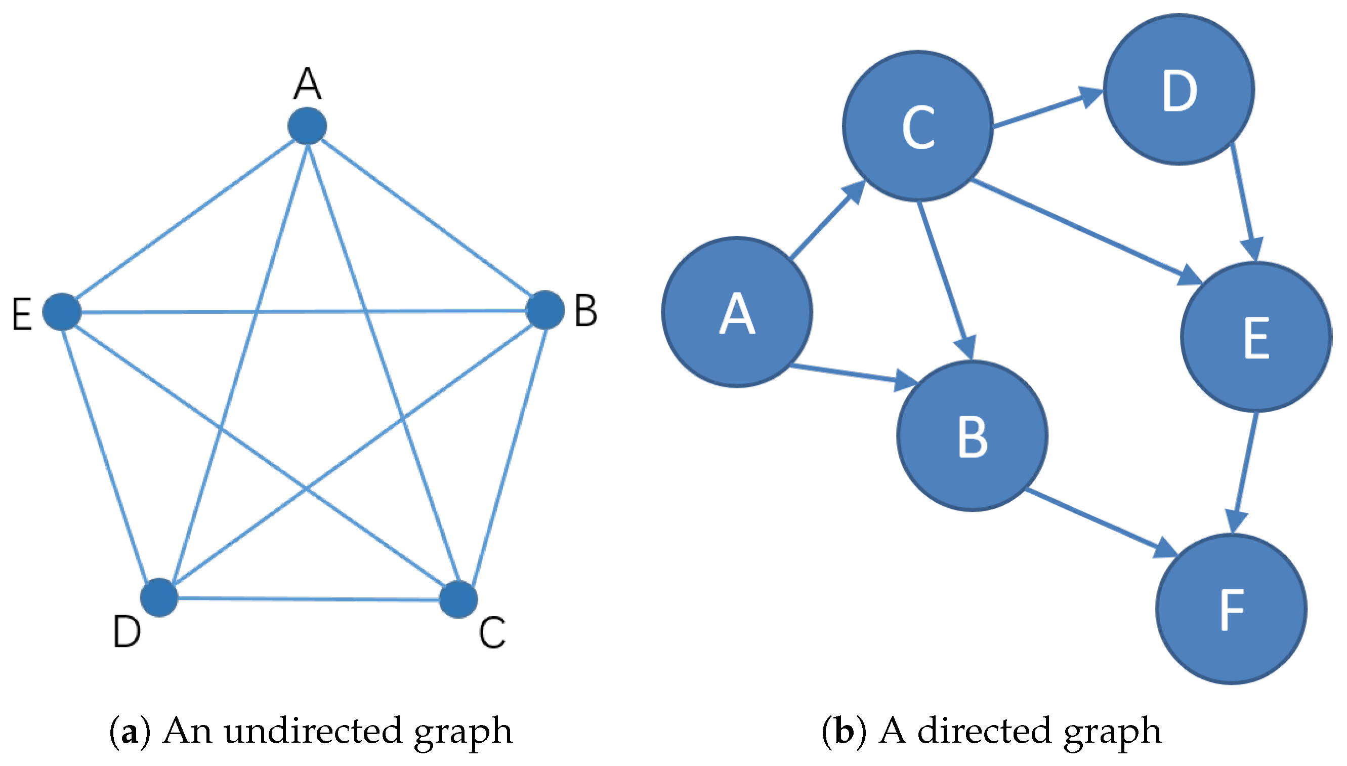
Definition 1

(Graph Concepts).A simple graph G is defined by a node-set V and a set E of two-element subsets of V, and the ends of an edge $uv$ are precisely the nodes u and v. A directed graph is a pair $\mathrm{D}=⟨V,E⟩$, where $\mathrm{V}=\left\{X_1,\dots ,X_n\right\}$ is the set of nodes and $\mathrm{E}=\left\{\left(X_i,X_j\right)|X_i,X_j\in V\right\}$ is the set of edges. Given that $\left(X_i,X_j\right)\in E$, $X_i$ is called a parent of $X_j$, and $X_j$ is called a child of $X_i$. The moral graph of a directed graph D is the undirected graph obtained by connecting the parents of all the nodes in D and removing the arrows. A loop in a directed graph D is a subgraph, whose underlying graph is a cycle. A directed graph is acyclic if it has no directed loops. A directed graph is singly-connected, if its underlying undirected graph has no cycles; otherwise, it is multiply-connected [11]. A graph G is $k-$regular if $deg\left(v\right)=k$ for all $v\in V$. A graph is bipartite if its vertex set can be partitioned into two subsets X and Y, so that every edge has one end in X and one end in Y [12].

Definition 2

(Bayesian Networks).Let $\mathrm{X}=\left\{X_1,\dots ,X_n\right\}$ be a set of random variables over multivalued domains $\mathcal{D}\left(X_1\right),\dots ,\mathcal{D}\left(X_n\right)$. A Bayesian Network (Pearl, 1988), also named a belief network, is a pair $<G,P>$, where G is a directed acyclic graph whose nodes are the variables X, and $P=\left\{P\left(X_i|p{a}_i\right)|i=1,2,\dots ,n\right\}$ is the set of conditional probability tables associated with each $X_i$. The Bayesian Network represents a joint probability distribution having the product form:

$$\mathrm{P}\left(x_1,\dots ,x_n\right)=\prod _{i=1}^{n}P\left(x_i|pa\left(X_i\right)\right)$$

Evidence E is an instantiated subset of variables $\mathrm{E}\subset \mathrm{X}$ [13].

Definition 3

(Loop Cutset).A vertex v is a sink with respect to a loop L if the two edges that are adjacent to v in L are directed into v. A vertex that is not a sink with respect to a loop L is called an allowed vertex with respect to L. A loop cutset of a directed graph D is a set of vertices that contains at least one allowed vertex with respect to each loop in D [13].

The loop cutset problem, for a directed acyclic graph $G=(V,E)$ and an integer k, is finding a set $S\subseteq V$, such that $\left|S\right|\le k$ and $G^{\prime }$ is a forest, where $G^{\prime }=\left(V,E^{\prime }\right),E^{\prime }=\{(u,v)\in E,u\notin S,v\notin S\}$. The problem can be transformed into a feedback vertex set (FVS) problem, as follows: convert the directed acyclic graph $G=(V,E)$ to its underlying graph. Subsequently, iteratively delete the nodes whose degrees are less than 2 and delete the adjacent edges. Denote the obtained undirected graph as $G_{new}=\left(V_{new},E_{new}\right)$, and then the problem involves finding a loop cutset $\mathrm{S}\subseteq V_{new}$ for $G_{new}=\left(V_{new},E_{new}\right)$.

Definition 4

(Conditional Independence).Let $V=\left\{V_1,V_2,\dots \right\}$ be a finite set of variables. Let $P(·)$ be a joint probability function over the variables in V, and let X, Y, Z stand for any three subsets of variables in V. The set X and Y are said to be conditionally independent, given Z if

$$P\left(x\right|y,z)=P(x\left|z\right)$$

In words, learning the value of Y does not provide additional information about X, once we know Z [12]. (Metaphorically, Z “screens off” X from Y.)

Definition 5

(d-Separation).A path p is said to be d-separated (or blocked) by a set of nodes Z if and only if (1) p contains a chain $i\to m\to j$ or a fork $i\leftarrow m\leftarrow j$, such that the middle node m is in Z, or (2) p contains an inverted fork (or collider) $i\to m\leftarrow j$ such that the middle node m is not in Z and, such that no descendant of m is in Z. A set Z is said to d-separate X from Y if and only if Z blocks every path from a node in X to a node in Y [12].

3. The Definition and Theorems of Shared Nodes

3.1. The Definition of Shared Nodes

Firstly, we define the shared node for two different nodes, in order to gauge the relativity and analyse the relationship between two nodes.

Definition 6

(Shared Node).For an undirected graph $G=(V,E)$, $v_1,v_2\in V$, if $e_1,e_2\in E$, $e_1=(v_1,v_i)$, $e_2=(v_2,v_i)$, then we call $v_i$ is one of the shared nodes of $v_1,v_2$. Similarly, in a directed graph $G=(V,E)$, $v_1,v_2\in V$, if $e_1,e_2\in E$, $e_1=(v_1,v_i)$ or $e_1=(v_i,v_1)$, $e_2=(v_2,v_i)$ or $e_2=(v_i,v_2)$, then we call $v_i$ is one of the shared nodes of $v_1,v_2$.

Figure 1 shows examples of shared nodes in directed and undirected graphs. In Figure 1a, the nodes A and B have three shared nodes: C, D, and E. In the complete graph, the shared nodes of any two nodes contain all the rest nodes. In Figure 1b, the nodes A and B have one adjacent edge and one shared node C, both of which can reflect the connection of two nodes. When two nodes have no adjacent edges and only shared nodes, such as in Figure 1b A and E, at this time, the message between the two cannot be directly transmitted through the adjacent edge, and needs to be transmitted through the shared node C or other longer paths. When two nodes have neither adjacent edges nor shared nodes, the messages between the two can only travel through a larger path, so that the influence between the two will be smaller. There is no shared node between the point with degree 0 and any other points.

Figure 1. An undirected graph and a directed graph. In (a), the nodes A and B have three share nodes: C, D and E; in (b), node A is a shared node between B and C.

The shared nodes show the connection of two different nodes, which are closely related to the measures of node centrality. They have practical significance in Bayesian networks: shared nodes are related to node-probability of loop cutset, which can be proved by theorems in Section 3.5; shared nodes are also related with two properties: conditional independent and d-separation, which are also discussed in Section 3.3.

3.2. Discussion on Shared Node and Node Centrality

The identification of which nodes are more “central” than others, or the centrality of nodes, has been a key issue in network analysis. Three different measures of node centrality were formalized Freeman in 1978: degree, closeness, and betweenness. Degree is the adjacent nodes number for a focal node, which is a straightforward index of the extent to which nodes are focus of activity. The index of the overall partial betweenness of the node is the sum of all its partial betweenness values for all unordered pairs of nodes. The closeness of a node, which is the sum of the number of edges in the geodesic linking the node and all th other nodes, determines its independence. A number of attempts have been made for generalizing the above measures. Barrat et al. extended degree to weighted networks, and Newman and Brandes made the extensions of the closeness and betweenness centrality measures in 2001.

Degree and path are commonly used in the measures of node centrality, such as in social networks and brain networks, and they have achieved the expected effect in actual applications. However, the actual application of the network model also needs to study the relationship between different nodes, such as the dynamic development of interpersonal relationships in the social network and the solution of the loop cutsets in Bayesian networks. More generally, thanks to the development of computers and algorithms, when solving a certain element, the algorithm is often iterative. In the iteration, the existing results should have a corresponding impact on the next calculation, so that the existing resources can be fully utilized.

Shared node and node centrality measures have a naturally close relationship: they both consider degree; both consider path; and, shared nodes and betweenness both consider the concept of a path between two points. Shared nodes are necessary and reasonable in measuring the relationship between two nodes.

3.3. Discussion on Shared Nodes and Conditional Independence

Shared nodes are related to conditional independence and directed separation, which are two important concepts of Bayesian networks. In Bayesian networks, conditional independence is a concept from the perspective of probability theory, and directed separation is a concept from the perspective of graph theory. Directed separation means conditional independence, according to the overall Markov property of Bayesian networks.

For three nodes $X,Y,Z$ in a Bayesian network, consider the four forms of Z as the shared nodes of X and Y: $X\to Z\to Y$, $X\leftarrow Z\leftarrow Y$, $X\leftarrow Z\to Y$, $X\to Z\leftarrow Y$, as shown in Figure 2a–d separately. For the situations in Figure 2a–c, the $XZY$ path is blocked by the node Z. In Figure 2d, the path will not be blocked, because the information from X will be missed at Z and it will not reach Y. If all the paths between X and Y are blocked by Z, then the node Z separates the nodes X and Y in a direction. If Z directed separates X and Y, when the variable in Z is observed, information cannot be transferred between X and Y, so X and Y are independent of each other, which is, X and Y are conditionally independent when Z is given. In these forms, the shared node plays a key role in judging whether two nodes are conditionally independent. In a Bayesian network, if two nodes X and Y are conditionally independent when a set C is given, then the set C contains all of the allowed shared nodes of X and Y.

Figure 2. The four forms of the node Z as one shared node of two nodes X and Y: (a) $X\to Z\to Y$; (b) $X\leftarrow Z\leftarrow Y$; (c) $X\leftarrow Z\to Y$; (d) $X\to Z\leftarrow Y$.

3.4. Study on the Shared Nodes Number between Different Nodes

The shared nodes reflect the relationship between two nodes and the number of shared nodes is a quantitative indicator of the relationship. The more shared nodes between two nodes, the closest the relationship. Below, we will study its upper and lower bounds of the shared nodes number and propose several theorems.

Theorem 1.

For an undirected graph $G=(V,E)$, denote the node with the largest degree $\Delta \left(G\right)$ of all nodes in the graph as $v_1$, the node with the next-largest degree ${\Delta }^{-1}\left(G\right)$ of all nodes as $v_2$, and the number of the nodes as n. Subsequently, for the shared nodes number ω between $v_1$ and $v_2$, the following inequality holds.

$$max\left(0,{\Delta }^{-1}\left(G\right)+\Delta \left(G\right)-n+1\right)\le \omega \le {\Delta }^{-1}\left(G\right)$$

Proof of Theorem 1.

We prove it in two cases: when the two nodes have adjacent edge and when they have no adjacent edge.

First, we degenerate the graph G to such a state: keep all of the nodes, keep all of the adjacent edges of the maximum degree node $v_1$, and remove all other edges. Suppose that we partition the space of variables V into three subsets $A,B,$ and C. Let A include node $v_1$ and its adjacent nodes, except node $v_2$, $B=V\backslash A\backslash v_2$, and $C=v_2$.

The subsets are shown in the Figure 3 and the following relations hold.

$$\begin{array}{c}\hfill A\cup B\cup C=V\\ \hfill \begin{array}{c}A\cap B=A\cap C=B\cap C=\varphi \\ \left|A\right|=\Delta \left(G\right)+1\\ \left|B\right|=n-\Delta \left(G\right)-2\\ \left|C\right|=1\end{array}\end{array}$$

Figure 3. The initial state of the graph G when the two nodes have no adjacent edge, where the set V is partitioned into three sets.

Consider the first case, which is, the two nodes $v_1,v_2$ have no adjacent edge. Subsequently, we can choose the $\Delta (-1)\left(G\right)$ adjacent nodes of $v_2$ from all nodes in sets A and B. In order to maximize the shared nodes number, we select all of the candidates from the set A, and the shared nodes number reaches the maximum value $\Delta (-1)\left(G\right)$. We select the candidates from set B until the selection cannot continue in order to minimize the number of shared nodes.

There are only two situations where the selection cannot be continued: no more nodes left to choose from B and still need to select the remaining adjacent nodes of $v_2$, i.e., $\left|B\right|<{\Delta }^{-1}\left(G\right)$; or, the selections have completed before set B is out of nodes, i.e., $\left|B\right|\ge {\Delta }^{-1}\left(G\right)$.

When $\left|B\right|>{\Delta }^{-1}\left(G\right)$, the shared nodes number $\omega$ between $v_1$ and $v_2$ is the adjacent nodes number minus the elements number of set B, which is:

$$\begin{array}{c}\omega ={\Delta }^{-1}\left(G\right)-(n-\Delta \left(G\right)-2)\hfill \\ \omega ={\Delta }^{-1}\left(G\right)+\Delta \left(G\right)-n+2\hfill \end{array}$$

where $\omega$ is an integer greater than zero. When $\left|B\right|<{\Delta }^{-1}\left(G\right)$, the value of $\omega$ is 0. At this time, the value of the expression ${\Delta }^{-1}\left(G\right)+\Delta \left(G\right)-n+2$ is an integer less than 0. Thus, when the two nodes have no adjacent edges,

$$max\left(0,{\Delta }^{-1}\left(G\right)+\Delta \left(G\right)-n+2\right)\le \omega \le {\Delta }^{-1}\left(G\right).$$

Consider the second case: the two nodes $v_1,v_2$ have an adjacent edge. At this time, among the ${\Delta }^{-1}\left(G\right)$ adjacent nodes of $v_2$, one is determined to be node $v_1$, and an edge $e_1=(v_1,v_2)$ exists in the initial graph, as shown in Figure 4. Subsequently, we can choose the $\left({\Delta }^{-1}\left(G\right)-1\right)$ adjacent nodes of $v_2$ from sets A and B, similar as in the first case. Finally, when the two nodes have no adjacent edges, the number of shared nodes satisfies the inequality: $max\left(0,{\Delta }^{-1}\left(G\right)+\Delta \left(G\right)-n+1\right)\le \omega \le {\Delta }^{-1}\left(G\right)$.

Figure 4. The initial state of the graph G when the two nodes have an adjacent edge, where the set V is partitioned into three sets.

In summary, the following inequality holds:

$$max\left(0,{\Delta }^{-1}\left(G\right)+\Delta \left(G\right)-n+1\right)\le \omega \le {\Delta }^{-1}\left(G\right)$$

 □

More generally, we can obtain the upper and lower bounds of the shared nodes number between any two nodes in a graph.

Theorem 2.

For an undirected graph $G=(V,E)$, denote the number of the nodes as n, and the degree of the node v as $deg\left(v\right)$. Afterwards, for $v_1,v_2\in V$, the shared nodes number ω between $v_1$ and $v_2$ satisfies the following inequality.

$$max\left(0,deg\left(v_1\right)+deg\left(v_2\right)-n+1\right)\le \omega \le min\left(deg\left(v_1\right),deg\left(v_2\right)\right)$$

Proof of Theorem 2.

The proof of Theorem 2 can use the same method of Theorem 1. We only need to replace the largest-degree node and the next-largest degree node with any two nodes, and the other parts still hold. Specific details will not be presented here.

Regular graphs and bipartite graphs are common network structures. A large number of regular and bipartite Bayesian network models can be found in application fields, such as turbofan jet engine gas path diagnosis, rocket engine sensor verification and diagnosis, computer network diagnosis, medical diagnosis, and code error correction. □

Theorem 3.

For any $n-$vertex, $k-$regular graph G, if the equality $k\ge \frac{n}{2}$ holds, then any two nodes have at least one shared node.

Proof of Theorem 3.

According to the definition of the regular graph, the degree of any node in G is k.

Because the equality $k\ge \frac{n}{2}$ holds, then, according to Theorem 2, the number $\omega$ of shared nodes between any two nodes satisfies the following relation.

$$\omega \ge {\Delta }^{-1}\left(G\right)+\Delta \left(G\right)-n+1=2k-n+1\ge 1$$

Thus, any two nodes have at least one shared node. □

Theorem 4.

Let $G=(X,Y,E)$ be an undirected bipartite graph, where $X=x_1,\dots ,x_n$, $Y=y_1,\dots ,y_m$ are two sets of vertices and E is the set of edges $x_i,y_j:x_i\in X,y_j\in Y$. For $v_1,v_2\in X$, denote the degree of $v_1,v_2$ as $deg\left(v_1\right),deg\left(v_2\right)$, respectively. The shared nodes number for $v_1,v_2$ satisfies the following relationship:

$$max\left(0,deg\left(v_1\right)+deg\left(v_2\right)-m+1\right)\le \omega \le min\left(deg\left(v_1\right),deg\left(v_2\right)\right)$$

Proof of Theorem 4.

The theorem can be proven by the definition of bipartite graph and Theorem 1. The proof process is similar to Theorem 1 and the details will not be given here. □

3.5. The Relationship between Loop Cutset and Shared Nodes

The conclusion mentioned above, that the number of shared nodes between two nodes is related to the probability that the two nodes belong to the cut set, is proven in this section. First, we give Lemma 1, cited from inference [8], which proves that the node degree influences the node probability of belonging to the loop cutset. Subsequently, Theorem 5 is proved according to Lemma 1 and the definition of loop cutset and shared nodes, which can explain the remaining problems in the experimental part of inference [8].

Lemma 1.

For an undirected graph $G=(V,E)$, any node $v\in V$ with $deg\left(v_2\right)\ge 2$, the probability that node v belongs to the loop cutset satisfies the following relationship:

$$p(v\in S)\ge 1-{\left(1-\frac{degv·(degv-1)}{(n_{nodes}-1)(n_{nodes}-1)}\right)}^{(n_{edges}-degv)}$$

where $n_{nodes}$ and $n_{edges}$ are the numbers of nodes and edges, respectively.

Theorem 5.

For an undirected graph $G=(V,E)$, $v_1,v_2\in V$, the probability that the nodes $v_1,v_2$ belong to the loop cutset is related to the number of the shared nodes between the two nodes. The greater the shared nodes number, the smaller the probability.

Proof of Theorem 5.

This theorem can be proven by Theorem 1 and the definition of the loop cutset. Once a node is selected into the loop cutset in a Bayesian network, then this node will be instantiated, in order to break as many loops in the network as possible. If two nodes are in one loop —and only one, then these two nodes will not be selected as loop cutsets at the same time. If two different nodes have many shared nodes, the two will be in more same loops, and the probability of both being selected in loop cutsets will be reduced. □

For the nodes $v_1,v_2$, having a shared node $v_i$ is equivalent to having a path of length 2, and $v_i$ is the intermediate node of this path. The greater the number of shared nodes, the more the number of paths with length 2 between the two nodes, and the closer the relationship. In fact, the number of shared nodes also implicitly reveals the shared part of the two degrees, which corresponds exactly to Lemma 1 and Theorem 1.

There is a question left in the experimental part of reference 2: the statistical probability of $r_{-}deg\left(v\right)$ has dropped significantly between 0.9 and 1, and the reason is to be discussed. In fact, the original motivation for defining shared nodes is to explain this phenomenon, and now Theorems 1 and 5 can explain it. First, when solving the loop cutset, the heuristic algorithms take the largest-degree node as the first element of the loop cutset, and the $r_{-}deg\left(v\right)$ of the largest-degree node has a value of 1. Next, consider the node with the next-largest degree, its $r_{-}deg\left(v\right)$ has a value that is closer to 1 than any other nodes. The number of shared nodes between these two nodes has a degree-related upper and lower bound, where the lower bound is $max\left(0,{\Delta }^{-1}\left(G\right)+\Delta \left(G\right)-n+1\right)$, according to Theorem 1. This lower bound is larger than any other two nodes in the graph. Subsequently, the probability that the two belong to the cut set at the same time will become smaller.

4. Experiments

This section implements four existing algorithms: the greedy algorithm A1 [3,4], the improved algorithm A2 [14] for A1, the MGA [5], and the WRA [6]. A large number of random Bayesian Networks are randomly generated using the algorithm in reference [4], and applied with the above algorithms. In WRA, we need to specify two constants: c and Max, and here we take the constant c as 1, and the constant Max as 300. The constant c influences the correct probability of the results, and the constant Max influences the solution speed. Four groups of Bayesian networks were randomly generated, in which the number of each group is 500, the number of nodes is 25, and the numbers of edges are 50, 100, 150, and 200, respectively. We applied the four algorithms to the networks.

We introduce the parameter $r_{-}deg\left(v\right)$ in order to measure the relative degree of one node in the graph, which is defined in reference [2]. Denoting the largest node degree in Graph G as $\Delta \left(G\right)$, and the degree of node v as $deg\left(v\right)$, the parameter $r_{-}deg\left(v\right)$ is the ratio ${\displaystyle \frac{deg\left(v\right)}{\Delta \left(G\right)}}$. In Figure 5, $r_{-}deg\left(v\right)$ is used as an independent variable. When $r_{-}deg\left(v\right)=1$, node v is the largest-degree node in G.

Figure 5. Statistical frequency of the $r_{-}deg\left(v\right)$ of nodes in the loop cutset (here, $n_{nodes}$, $n_{edges}$ are the numbers of the nodes and edges, respectively).

Figure 5 shows the relationship between the $r_{-}deg\left(v\right)$ of the node and the corresponding statistical frequency of different $r_{-}deg\left(v\right)$. We obtained the trend that the statistical frequency increases with the parameter $r_{-}deg\left(v\right)$ increasing, which is more obvious when the graph is more complicated. However, there is a significant decline in the statistical frequency near the value of 0.9 for $r_{-}deg\left(v\right)$ in each graph, which verifies the conclusion of Theorem 5.

The results are consistent with the conclusion of Theorem 5. Because, in the algorithms A1, A2, and MGA, the first choice is the node with the largest degree in the graph, and the $r_{-}deg\left(v\right)$ of the largest degree node is 1. Thus, the statistical frequency at the $r_{-}deg\left(v\right)$ value of 1 maxes. As the largest-degree node has been selected into the loop cutset, and the nodes in the loop cutset will be instantiated, the messages from the largest-degree node will be spread along its neighboring nodes. The other node receives information from the largest-degree node through shared nodes between them. The more the shared nodes, the more information received; thus, the smaller node-probability of the loop cutset. According to Theorem 1, the shared nodes number between the largest-degree and next-largest degree nodes is greater than the constant $max\left(0,{\Delta }^{-1}\left(G\right)+\Delta \left(G\right)-n+1\right)$, where $\Delta \left(G\right)$ is the largest degree, ${\Delta }^{-1}\left(G\right)$ is the next-largest degree, and n is the number of the nodes in the graph. Thus, the node-probability of the next-largest degree will be reduced, which can explain the sudden drop in statistical frequency in Figure 5.

Next, we study the shared nodes number between two nodes in the loop cutset, to examine the relationship between the shared nodes number and the probability of two nodes that belong to the loop cutset. Figure 6 shows the statistical probability of two nodes belonging to the loop cutset according to different shared nodes number, where the nodes number is 25 and the edges number is 50, 100, 150, and 200, respectively. It can be seen that, the larger the shared nodes number, the smaller the frequency of two nodes belonging to the cut set, which corresponds exactly to Theorem 5.

Figure 6. Statistical probability of the shared nodes number in the loop cutset (here $n_{nodes}$, $n_{edges}$ are the numbers of the nodes and edges respectively).

We introduce a parameter ${\Theta }_{p,q}$ defined in Reference [8] in order to describe the degree of edge-saturation in the graph. Assuming that a simple graph $G=(V,E)$, the nodes number is p, and the edges number is q, then p and q satisfy the relationship $\mathrm{q}\le \frac{1}{2}p(p-1)$. The parameter ${\Theta }_{p,q}$ is defined as ${\Theta }_{p,q}=2q/p(p-1)$. The value-range of ${\Theta }_{p,q}$ is $[0,1]$, and when its value is 0, G is a trivial graph; when its value is 1, G is a complete graph. It can be seen from this definition that the parameter ${\Theta }_{p,q}$ can describe the degree of edge-saturation in the graph, and measure the complexity of the graph from the perspective of the edge-saturation.

When the nodes number is 25 and the edges number is 50, 100, 150, 200, the values of ${\Theta }_{p,q}$ are 1/6, 1/3, 1/2, 2/3, respectively. As can be seen from Figure 6, as the value of ${\Theta }_{p,q}$ keeps increasing, the complexity of the graph is getting bigger, and the shared nodes number of the nodes in loop cutset are getting bigger. This shows that, with the increase of edge-saturation, the node-to-node ties have become closer.

5. Extended Applications of Shared Nodes

Because the shared node is related to the node-probability of the loop cutset, then we can use this conclusion in the loop cutset solving algorithm. When using the greedy algorithm to solve the loop cutset, the obtained members of the loop cutset should have an impact on the candidate nodes in the next step. We formulate the strategy of “least shared nodes”: when looking for the next candidate node, in addition to applying the existing maximum degree strategy and the least sample space strategy, we also consider the least number of shared nodes with the obtained members of the loop cutset. This strategy can be applied to the existing two classes of loop cutset algorithms: heuristic algorithms and random algorithms.

Next, we briefly explain the improvement with the application of the "least shared nodes" strategy in the heuristic algorithm. For the initial graph that is shown in Figure 7a, node 0 is selected as the first element of the loop cutset. Then graph Figure 7b is obtained after the elimination of node 0, in which node 1 and 2 has the same degree of 4. In the greedy algorithm A1 and its improved algorithm A2 [3,4], the heuristic strategy has the following three components: firstly, only those nodes that have one or no parents are considered; secondly, the node with the most neighbours of that remain under consideration are selected; thirdly, select the node with the lowest number of possible values of that remain under consideration [4]. In the graph that is shown in Figure 7b, we cannot confirm the next candidate based on the above heuristic strategy. However, considering the “least shared nodes” strategy, we can choose node 2 as the next element of the loop cutset, which has the less shared nodes with node 0 and cuts more loops than node 1. The above example briefly applies the “least shared nodes” strategy, and it also shows that the “least shared nodes” strategy can optimize the solving algorithms of the loop cutset.

Figure 7. For the Graph in (a), node 0 is selected as the first element of the loop cutset. Then graph (b) is obtained after the elimination of node 0, in which node 1 and 2 has the same degree of 4. When considering the “least shared nodes” strategy, we choose node 2 as the next element of the loop cutset, which cuts more loops than node 1.

In the social network, the shared nodes also reveal the relation between different persons. In such a network, if a node is used to represent a person and the edge between two nodes is used to represent the acquaintance, then the shared nodes between two nodes means the persons that they know together. If the social network is dynamic, when there is no direct relationship between two people, the more people they know together, the greater the probability that they may know each other later. Thus, the number of shared nodes indicates the intimacy of the social relationship between the two, and it also indicates the probability of subsequent recognition.

6. Conclusions

We have provided a new tool to gauge the relationship between different nodes—shared nodes, proven the upper and lower bounds of the shared nodes number, revealed the relationship between the shared nodes number and the node-probability of the loop cutset. We show that the experimental results support the correctness of the theorems in this paper. Moreover, we present an optimal to the existing algorithms for solving the loop cutset, and discuss extended applications of shared nodes in the social network.

The proposal of shared node attempts to measure the relationship between two nodes, which is necessary in many practical applications. The shared node’s measure of the relationship between two nodes is related to the measures of the node centrality—they both contain the concepts of degree and path, so they are reasonable. More generally, with the development of computers and algorithms, the algorithm is often iterative to solve a certain element. In the iteration, the existing results should have a corresponding influence on the next calculation, so that the existing resources can be fully utilized. In this way, the relationship between the two is the answer to the question that we want to know.

However, potential future research with the shared nodes exists based on our theoretical analyses: the proposition that the shared nodes are related to conditional independence and graph measurement lacks exact proof and data support; the applications of shared nodes in algorithms and network analysis can be further implemented.