Abstract
The switched reluctance machine (SRM) design is different from the design of most of other machines. SRM has many design parameters that have non-linear relationships with the performance indices (i.e., average torque, efficiency, and so forth). Hence, it is difficult to design SRM using straight forward equations with iterative methods, which is common for other machines. Optimization techniques are used to overcome this challenge by searching for the best variables values within the search area. In this paper, the optimization of SRM design is achieved using multi-objective Jaya algorithm (MO-Jaya). In the Jaya algorithm, solutions are moved closer to the best solution and away from the worst solution. Hence, a good intensification of the search process is achieved. Moreover, the randomly changed parameters achieve good search diversity. In this paper, it is suggested to also randomly change best and worst solutions. Hence, better diversity is achieved, as indicated from results. The optimization with the MO-Jaya algorithm was made for 8/6 and 6/4 SRM. Objectives used are the average torque, efficiency, and iron weight. The results of MO-Jaya are compared with the results of the non-dominated sorting genetic algorithm (NSGA-II) for the same conditions and constraints. The optimization program is made in Lua programming language and executed by FEMM4.2 software. The results show the success of the approach to achieve better objective values, a broad search, and to introduce a variety of optimal solutions.
1. Introduction
The switched reluctance machine (SRM) is the type of machines that develop output torque due to reluctance variation without using permanent magnets or rotor excitation. The switching of phases is made according to position of rotor in such a way to produce torque (induce voltage in generation mode). Reluctance variation happens with rotation as a function of certain geometric parameters. The currents of SRM are mainly in the form of pulses. The flux inside the machine is not sinusoidal. All of the previously mentioned facts of SRM give this type of machines its unique features. The SRM has shown attractive characteristics, such as simple and robust construction, low manufacturing cost, and high efficiency, over wide range of speeds [1,2]. SRM’s construction simplicity and low manufacturing cost have motivated both researchers and manufacturer.
However, the pulsative behaviour of currents results in torque ripples that are considered a problem of SRM and a challenge. The saliency of poles and non-sinusoidal wave-forms of flux in SRM result in noisy operation and radial vibrations. In addition, SRM structure is not simple from geometric perspective due to the wide range of probabilities for dimensions of a certain design. Moreover, the relationships between SRM’s geometric parameters and performance indices are indirect and non-linear. Hence, the search for a good design is difficult despite the search for the best (optimal) design.
Optimization is the search for the best solution (the optimal solution) for a certain problem [3]. Various types of optimization algorithms exist, including traditional optimization techniques that have many limitations and advanced population-based meta-heuristic algorithms [4,5,6]. Optimization is needed with a switched reluctance machine (SRM) design to reach better designs. Sensitivity analysis is the study of the degree of influence of each parameter on the final objectives of the design. Subsequently, the most influencing parameters are chosen to be optimized to save computation time. Because of the large number of geometric parameters or design parameters of SRM, sensitivity analysis is usually made to make the optimization process less complicated, as in [7,8,9].
It is essential to have a mathematical model of SRM in order to evaluate its performance and include this evaluation in the optimization process. The performance of SRM is mainly evaluated by rated torque, torque per weight, torque per volume, rated speed, and efficiency. Other quantities can be added to give more detailed evaluation, such as torque ripples, acoustic noise, mechanical vibrations, and maximumtemperature rise, and so forth. All of these performance indices are calculated by various methods that differ from each other according to their accuracy and computational time. These method can be classified to numerical methods, such as finite elements analysis (FEA) and boundary element method (BEM), and analytical methods, such as curve-fitting methods, magnetic equivalent circuits (MECs), and Maxwell’s-equation-based approaches [1]. Numerical methods provide high accuracy with the cost of its high computational time. Analytical methods can be simplified to achieve a fast calculation process. However, in most cases, this results in a reduction of accuracy. FEA is commonly used in SRM modelling to achieve accurate results, as in [10,11,12,13,14]. Magnetic equivalent circuit (MEC) is faster than FEA, as shown in in [15,16,17]. However, it is less frequent because of its reduced accuracy. Fuzzy logic and regression methods are also used, as shown in [18,19]. However, they are less reliable and have complex structures when compared with FEA and MEC. Each performance index (i.e., rated torque, torque ripples and so forth) of SRM is called “objective function” when it is used in the optimization process.
Each possible solution (candidate) of the optimization problem has a corresponding objective function value. According to this value, the candidate solution is ranked. Solution Optimization techniques may be classified according to the objective of optimization into single-objective and multi-objective. In single-objective optimization techniques, only one objective function is considered and solution candidates are ranked based on their corresponding objective function value. For example, if it is required to maximize the objective function, the optimal solution is the one that results in the maximum value of objective function (and vice versa). In multi-objective optimization techniques, more than one objective functions are considered and solution candidates are treated in a different way, as will come later. Multi-objective optimization provides a set of optimal solutions instead of one in single-objective optimization. Optimization techniques have been used together with a modelling method to obtain optimal designs. The enumeration optimization method with FEA is used in [20,21,22]. A genetic algorithm with FEA is used in [10,13,14]. In [18], a genetic algorithm is used with fuzzy logic. The non-dominated sorting genetic algorithm (NSGA-II) method is used in [23] with FEA. Differential evolutions are used in [24,25] with FEA. Particle swarm optimization (PSO) is used in [26,27,28,29] with different SRM modelling techniques. The increase in computation time in most approaches is due to time-consuming SRM electromagnetic modelling. Using other methods instead of FEA is even less accurate or complicated to build.
In this paper, FEA is chosen for SRM modelling to complement the mathematical formulas for average torque and core losses calculations. FEA usage is limited to inductance calculation and to obtain flux density for some points inside SRM core. This simulation has proved to be achieved in a very short time while using free software FEMM4.2. Accordingly, the computational time is reduced to an acceptable limit while achieving high accuracy. The Jaya algorithm is introduced to optimize SRM design due to its inherent characteristics, as it takes the path directly toward optimal solutions, saving computational time and achieving better objective functions values [30]. The multi-objective version of Jaya (MO-Jaya) algorithm is considered with three objective functions, and they are rated average torque, efficiency, and iron weight. The three objective functions calculation methods are presented in details. The results of optimization and the performance of the Jaya algorithm are compared with those of the non-dominated sorting genetic algorithm (NSGA-II) under the same constraints and for the same objectives [31]. The proposed method represents a general frame work for SRM multi-objective optimization. Unlimited design parameters and objective functions can be included. The objective of this study is to investigate the performance of MO-Jaya algorithm in SRM design optimization.
2. Design of SRM
Before starting the design process of switched reluctance machine, available space should be well investigated. The available space is represented as constraints of SRM dimensions values. The most important space constraints are axial length, maximum outer diameter (maximum frame size), and shaft diameter. The axial length and maximum frame size are obtained from measurements of the available space. The shaft diameter is calculated based on the maximum torque and speed. The difference between maximum outer diameter and Shaft diameter is the space that is available for SRM cores and turns. SRM cores are the stator and rotor, which are salient in producing reluctance variation. The number of poles in both stator and rotor is specified at the beginning as will come later.
In conventional design approaches, lamination dimensions, coil diameter, and number of turns are calculated analytically. Subsequently, the average torque is calculated and compared with the rated required torque. The average torque is calculated based on the flux-current () curves for aligned and unaligned positions. Finally, the whole process is repeated with modified dimensions values and the number of turns to match the output average torque with the required torque. Other performance indices can also be considered, such as torque ripples, efficiency, and so forth. This section demonstrates calculation methods of the considered performance indices and characteristics.
2.1. Number of Poles Selection
Stator poles number and rotor poles number is specified mainly according to general understanding of their influence on SRM performance. A higher pole number produces higher average torque, lower torque ripples, and provides more reliable operation; however, it requires more switching devices and reduces the maximum speed. Lower poles number produces lower average torque and higher torque ripples; however, it requires less switching devices and provides higher maximum speed. For general purpose SRM design, 6/4 and 8/6 SRM configurations are commonly used. Hence, these two configurations are considered for optimization in this paper.
2.2. Poles Arcs Calculation
When considering , are stator pole arc and rotor pole arc, respectively. To achieve self-starting SRM design, minimum stator pole arc may be expressed—as in [32]—by:
The following condition prevents overlap between phases:
If this condition not being followed, then the SRM machine inductance will start to increase before reaching the minimum inductance value. This results in higher unaligned inductance value and the developed torque becomes lower.
2.3. Main Dimensions
Referring to Figure 1 and Table 1, the maximum value of outer diameter () and maximum value of axial length (L) are obtained from space constraints. Shaft diameter () is obtained from the shaft’s standard sizes that are based on output torque value. The values of outer diameter () and axial length (L) can be changed during design within their maximum values. However, keeping them at their maximum values results in the maximum output torque of SRM design. The shaft diameter () is kept constant during design process. The air gap length (g) is assumed to have the commonly used value of mm that can be obtained often in practical implementation. The rest of the dimensions are modified to reach the requirements of design.
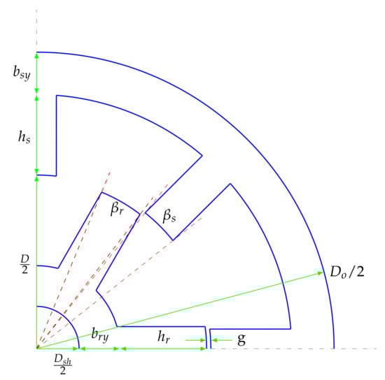
Figure 1.
The lamination dimensions considered in the optimization process.

Table 1.
SRM dimensions.
2.4. Variables Dimensions Limits
The limits of variables are determined by the application and the available space. In this paper, outer diameter (), axial length (L), shaft diameter (), and air gap length (g) are kept constant by making their maximum and minimum limits at the same value. The remaining limits are set by the previous experience. Table 2 shows the maximum and minimum limits values of all the variables.
Table 2.
Limits of variables.
2.5. Winding Design
Winding design is achieved, as in [31,33]. The number of turns per phase is calculated based on SRM dimensions, such that the flux density value at the knee point of iron’s B-H curve is maintained. In this paper, the value of maximum flux density for the used lamination steel is 1.65 T.
The conductor cross-sectional area is calculated from a specified maximum ampere and current density. Subsequently, the number of horizontal layers, vertical layers, and coil dimensions can be calculated. Finally, clearance between adjacent coils is calculated at the point where the two coils are the closest to each other [31].
2.6. Average Torque Calculation
The SRM average torque is calculated based on assuming that flux linkage () vs. current (i) characteristics are available and the phase current is kept constant at its peak value between unaligned and aligned positions [32]. The average torque is calculated from the total work done of all strokes for one revolution, as follows:
where and are the areas under curves at the aligned position and unaligned position, respectively. W is the area of energy loop between two curves and calculated as in [32].
2.7. Efficiency Calculation
It is essential to know the losses of switched reluctance motor in order to calculate efficiency [34]. SRM losses calculation, especially the assessment of core losses, is a very difficult task mainly due to tha fact that flux wave-forms are non-sinusoidal and different from each other based on the sector that they are located in SRM’s magnetic circuit. Moreover, core losses are dependent on the type of control and operating speed (). In a low speed region, it is acceptable to neglect the mechanical losses. Hence, losses may be calculated as:
Once the losses are known, the efficiency may be calculated by:
In this paper, efficiency is calculated at the rated speed of 1000 rpm for all SRM designs candidates.
2.8. Copper Losses
Copper losses value depends on phase current, which is determined by the control technique. When considering that is number of phases, is phase dc resistance, and is phase current, the total copper loss instantaneous value may be calculated by the equation:
The average copper losses can be calculated by equation:
where T is the period of time for strokes. For sake of simplification, we assume no overlap between phases. Because the current of phase is not pure dc. The peak value of it () is considered for copper losses calculation as a pessimistic prediction. Copper loss is then calculated straight forwardly by the equation:
2.9. Eddy Currents Losses
Referring to [35], the eddy current losses in SRM can be calculated by the equation:
where e: sheet thickness in meter, : constant () introduced to account for the fact that paths in the interior of the lamination will have smaller emfs than those that are near the surface; : the electrical resistivity of the ferromagnetic material (in ); : density of the ferromagnetic material (in ).
From Equation (10), the waveform of flux density (B) for all SRM sectors must be known. Once they are available, is calculated by numerical integration and differentiation. There are a lot of methods to obtain these wave-forms and many of them are time consuming. In [34], a mathematical method using matrices is introduced in order to obtain the wave-forms of all the SRM sectors in a systematic manner. The calculation of B wave-forms for all sectors is achieved by the modulation of triangular pulses. The stator poles wave-forms only consist of unipolar triangular pulses, while those of the rotor poles contain both positive and negative pulses. The stator and rotor yoke wave-forms have a more complicated relationship with the triangular pulses. This method is demonstrated in details in [34] and then used here for 8/6 and 6/4 SRMs.
2.10. Hysteresis Losses
Referring to [31], the hysteresis losses can be calculated for various sectors of SRM. The flux density wave-forms depend on the phase current waveform and the speed of the motor. The flux density wave-forms calculated in this paper rated the speed of 1000 rpm and control is by a single pulse voltag. Note that the phase current has the peak of six ampere for all SRMs design candidates.
3. Jaya Optimization Method
The population-based meta-heuristic optimization algorithms can be classified to two groups, and they are the evolutionary algorithms (EA) and swarm intelligence (SI) based algorithms. All of these algorithms have the same basic structure that is explained by Figure 2. Firstly, the initialization of solutions in the beginning is made mainly by random choice of variables. Then, the objective function values are obtained and evaluated. After that, selection of the best solutions is made to use these solutions in the production of new solutions. Finally, the termination condition of the process is checked if true, and then end or else continue.
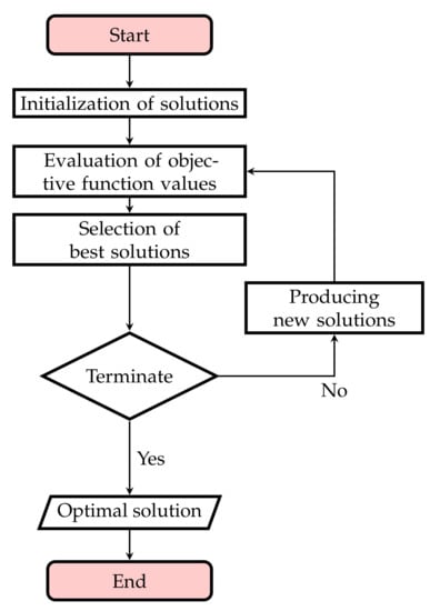
Figure 2.
Flowchart of general optimization algorithm.
Optimization techniques differ from each other by the different methods that are used to accomplish these steps. However, all of population-based meta-heuristic optimization algorithms have a common limitation, which is the different parameters that are required for proper working.
Referring to [30], the Jaya algorithm was introduced in 2016 by Ravipudi Venkata Rao. "Jaya” is a Sanskrit word that means victory or triumph. The algorithm is simple to implement and it does not require tuning of any parameters. In Jaya algorithm, the initial solutions are randomly generated within the search space. After that, the solutions are updated using Equation (11).
where b and w represent the index of the best and worst solutions in the population. are the index of iteration, variable, and candidate solution, respectively. is the jth variable in ith iteration of kth solution candidate. are random generated ratios in the range of to ensure good diversification.
3.1. Single Objective Jaya Algorithm
In single objective optimization, the required is to maximize or minimize a single function. Thereby, for two solution candidates a better solution is whether greater or smaller in value. For objective function , which has m variables and n population size, the solutions are represented by a data structure i.e., matrix as in Equation (12). Each solution may be represented by a column of different variables. The objective function () can be represented by a matrix (F) that has one row and n columns in the case of single objective optimization, as in Equation (13). For multi objective optimization problem with number of q objective functions, matrix F is of q rows and n column as in Equation (14).
Solution matrix (X) is updated using Equation (11) based on the best and worst solutions obtained by comparing all of the solution candidates with each other.
3.2. Multi Objective Jaya Algorithm
Solutions in multi objective Jaya algorithm are updated using the same Equation (11), and the results of objective functions are represented in Equation (14). However, non-dominated sorting approach and crowding distance computation mechanisms are to be used in order to handle the conflicting objectives of optimization problem. It is essential Jaya algorithm to obtain the best and worst solutions in order to produce new solutions using Equation (11).
In multi objective optimization problem, obtaining the best and worst solutions is not straightforward as in single objective optimization. After non-dominated sorting is achieved and crowding distances are computed for solutions of the same rank (front), the best solution would surely be in the first rank and the worst solution would be in the last one. However, the solutions of the same rank cannot be compared with each other and, hence, the crowding distance is used to decide the best and worst solutions among their ranks. The crowding distance is an indicator of the degree of diversity of solutions in same front; hence, solutions with higher crowding distance are preferred, which enables covering a wider search area. In [30], the solution with highest crowding distance among first rank solutions is considered to be the best and the solution with the lowest crowding distance among last rank solutions is considered to be the worst.
In this paper, the other method is used to decide the best and worst solutions. The best solution is chosen randomly from the first rank, this choice is changed four times until all population solutions are updated. In the same manner, the worst solution is chosen randomly from the last rank. This method achieves a wide variety of solutions by distributing the priority of search among different search directions. Finally, the designer has the option to choose the best design that serves the application among best ranks of solutions.
Dominance
It is required to check each solution with the rest on the dominance basis. Assuming that are two solutions, m is the number of objective functions, if ( dominates ) is true, the Pareto dominance conditions must all be true, and they are:
Dominance is investigated for all of the solutions. The solution that is not dominated by any of the remaining solutions is a non-dominated solution and it is removed from the solutions matrix. This is repeated for all solutions and the resulted non-dominated solutions are considered rank 1. The same process is repeated for the remaining ranks.
Crowding Distance
Crowding distance is computed in the same manner, as mentioned in [30] (page 15). Crowding distance is computed for each solution using Equation (15).
where j is a solution in the sorted list, is the objective function value of mth objective, and and are the population-maximum and population-minimum values of mth objective functions.
4. Multi-Objective Jaya Algorithm for SRM Design Optimization
In the optimization of SRM, the dimensions in Table 1 represent one solution. All of the solutions are stored in the matrix (X), as follows:
where m is the number of variables and n is the size of population in one generation.
4.1. Objective Functions
The objectives of SRM optimization depend on the application and its conditions. For general purpose SRM, average torque and efficiency are needed to be maximized and iron weight is to be minimized. In some applications, other objectives (i.e., torque ripples, acoustic noise, vibrations ⋯, and so forth) are considered.
4.2. Constraints
Because the SRM dimensions are significant, there must be certain constraints on them to prevent any non-logical vector of variables. The dimensions in variables matrix (X) must be modified to satisfy the following constraints:
It is also a part of the constraints to specify certain limits to each variable(dimension). If a certain dimension needed to be fixed, this can simply achieved by setting both the minimum and maximum limits to the desired value.
Code Algorithm
The code is made using Lua programming language. The code is executed by FEMM4.2 software. The choice of Lua programming language to be used is due to its simplicity, and that it is adopted by FEMM4.2, which provides the FEA analysis in good accuracy. Figure 3 shows the code’s algorithm. The code starts with inserting SRM optimization data. These data include the population size, problem variables, variables limits, and objective functions, to specify which objective function to maximize and which to minimize, maximum iterations limit and numbers of rotor and stator poles ( and ). Subsequently, solutions initialization are achieved for all solutions in the population by a random choice of variables within the search space that is stored in matrix X as in Equation (16). After that, the solutions are modified to satisfy constraints in Equations (18)–(21) by changing the values of variables that resulted from random choice. This change is to give the variable that is out of its limits one of the acceptable limits value. For example, if a variable is greater than maximum, then it is changed to the maximum value and vice versa. Subsequently, FEA Analysis is accomplished using FEMM4.2 software to calculate average torque, maximum stator and rotor poles flux densities and volume of iron. Next, remaining objective functions ( and ) are calculated using the results of FEA analysis. After that, non-dominated sorting is achieved and crowdingdistance is calculated for all fronts. Based on non-dominated sorting and crowding distance, the best and worst solutions are specified. Susequently, the termination condition is checked if the number of iterations exceeds the maximum limit or not. Finally, output of optimization is provided, which is the non-dominated front of all solutions. Note that the output also provides all solutions that have been produced for all iteration, which is beneficial to provide more solutions for designer to choose.
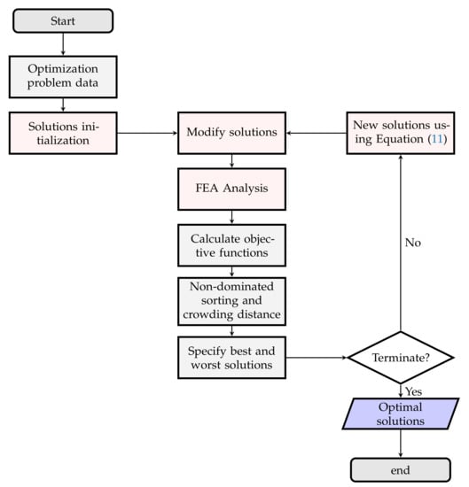
Figure 3.
Flowchart of MO-Jaya algorithm.
5. Results and Discussions
The evaluation of optimization algorithm performance may be mainly achieved by two factors that are computational time and candidates. The less computational time, the better is the performance for the same results of candidates. On the other hand, the better candidates, the better performance for the same computational time. In this paper, better candidates production are of significant interest than computational time. SRM design candidates with higher average toque and efficiency and lower iron weight are considered to be better candidates. Hence, it is expected that for a successful optimization process, most of the search (crowded area) ought to be in the areas that maximize both average toque and efficiency and minimize iron weight. For example, assuming that it us desired to maximize both of objective functions and , the results of the optimization process that are the solution candidates should be at the upper right quarter, as shown in Figure 4. The same goes for other quarters in cases of minimizing both and , maximize and minimize , and maximize and minimize . Additionally, it is expected that the optimization program will find more solutions in the correct quarter (direction) with increased iterations until the search area is fully covered.
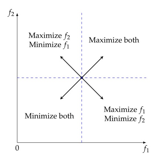
Figure 4.
Search directions in multi objective optimization.
The objectives of optimization in this paper are to maximize average torque () and efficiency () and minimize iron weight (). The results of optimization process are considered in pairs, as shown in Figure 5 and Figure 6. In Figure 5c, efficiency is increased and iron weight is decreased while iterations are increasing. The search direction is correct according to Figure 4. The search direction is also correct with respect to iron weight and average torque, as shown in Figure 5b. In Figure 5a, the search direction is not clearly obvious, as in Figure 5b,c, which is due to the non-linear relationships of dimensions and objective functions (efficiency and average torque). The program changes the direction to cover all the search area to provide a various groups of solutions.
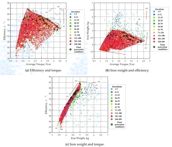
Figure 5.
Objective functions results for 8/6 SRM.
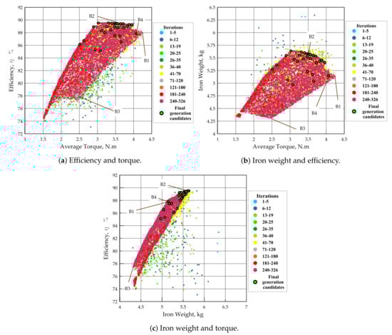
Figure 6.
Objective functions results for 6/4 SRM.
In Figure 7, objective functions of SRM are shown with respect to the number of iterations. It can be seen that the objectives are conflicting with each other. The optimization program is made, such that the iterations are continued while the algorithm is not biased for any of the objectives by changing the best and worst solutions in the way mentioned earlier in Section 3.2. Hence, better solutions are found in all of search directions (objectives). Figure 8 shows how objective functions interact with each other and confirms the wide search area.
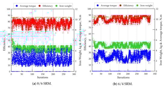
Figure 7.
Objectives with iterations for 8/6 and 6/4 SRM using MO-Jaya.
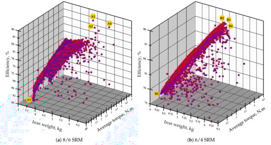
Figure 8.
3D representation of objective functions values through optimization process.
Every point represents a solution and some solutions are invalid due to dimensions constraints, as they cause a negative clearance between windings. The penalty for these solutions is to eliminate them by making their corresponding objective functions the worst of their values. Hence, the invalid solutions take zero average torque and efficiency and iron weight of the whole volume (), where is the density of iron.
It can be seen that search direction is changing while iterations increases as the ups and downs in objective functions values indicate. In other words, the program is exploring new areas with more iterations. This is because of two reasons, the first reason is the random chosen ratios and in Equation (11). The second reason is the random choice of the best and worst solutions from the highest and lowest ranks (fronts). This is beneficial, as the algorithm does not repeat it self and provide more various solutions. However, a drawback is that optimal solutions (non-dominated front) are distributed over iterations. In other words, the best candidates do not exist in the last iteration exclusively. The designer then has to take this into consideration while choosing a design to implement.
For further evaluation, the optimization results by multi-objective Jaya algorithm (MO-Jaya) are compared with optimization results by non-dominated sorting genetic algorithm (NSGA-II) in [31]. Two optimization processes have the same constraints, objective functions, calculation methods, and common parameters (population size and maximum iterations). The results that are shown in Figure 5, Figure 6 and Figure 7 in this paper are compared with results that are shown in Figures 4, 5k and 7 in [31]. The comparison can be summarized in the following point:
- It can be seen that MO-Jaya provides much better coverage of search area. The results in [31] are more concentrated in small area. The reason for this is the constant parameters of cross over and mutation in NSGA-II method, unlike MO-Jaya, where the parameters are randomly changed. This is obvious by comparing Figure 5 and Figure 6 in this paper with Figures 4 and 5 in [31].
- Figure 7 in this paper shows that the optimal solutions may be lost with increased iterations, unlike in [31], as shown in Figure 5. This is a consequence of changing direction of search, as demonstrated earlier. This has no effect on the total design candidates that Jaya algorithm provide and the designer can choose various design candidates from any iteration’s population.
Four optimal solutions are chosen for both 8/6 and 6/4 configurations. Table 3 summarizes the selected designs and their corresponding objective functions. Most of designs do not belong to the last iteration, as they provide better characteristics. For 8/6 SRM configuration, design A1 achieves the highest average torque, A2 achieves highest efficiency at rated speed, A3 has the lowest iron weight, and A4 is a compromise design which gives a higher priority for average torque and efficiency. For the 6/4 SRM configuration, design B1 achieves both the highest average torque and efficiency at rated speed, B3 has the lowest iron weight, and B2 and B4 are the compromise designs. Figure 5 and Figure 6 show the location of the selected designs among the remaining designs. It is worth mentioning that the resulted optimal designs by Mo-Jaya optimization method are close to these that result from NSGA-II for the same constraints. However, the Mo-Jaya method achieved better diversification than NSGA-II.
Table 3.
Chosen optimal candidates.
Table 4 shows the details of selected designs. It can be noticed that the parameters and dimensions of SRM are changed with iterations to produce better designs in such a way that matches with the SRM design experience. This indicates that the calculation methods of objective functions mainly succeeded to represent SRM. For example, when rotor pole length () is increased and rotor yoke thickness () is reduced, the impact on SRM is to produce average torque. This result matches with design experience, as the difference between anligned and unaligned inductances is increased and, hence, energy conversion increases Equation (4).
Table 4.
Parameters and objective functions values of the selected optimal designs.
Torque per phase is shown in Figure 9 for 8/6 and 6/4 SRM configurations before and after optimization. The peak torque is increased in optimal designs (A1 and B1) over initial designs. It can be also noticed that torque ripples also increase. This is because torque ripples minimization is not considered as an objective for optimization. However, so far, the program succeeded in achieving what is requested and specified in the objectives. More work is taking place to include torque ripple minimization in optimization objectives in the future.
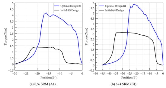
Figure 9.
Torque per phase of initial and optimal SRM designs.
Further study on selected SRM design candidates are made to evaluate efficiency over a wide range of speeds Figure 10. It can be noticed that 6/4 SRM (B group) achieves higher efficiency values. This is due to lower iron losses that are caused by flux variation in magnetic circuit of SRM. Figure 11 shows the iron losses.
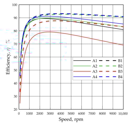
Figure 10.
Efficiency over wide range of speeds.
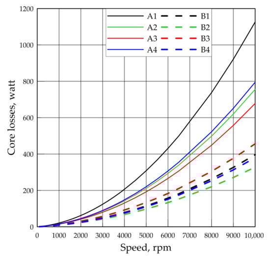
Figure 11.
Core losses of selected optimal designs over wide range of speeds.
6. Conclusions
In this paper, the Jaya algorithm is introduced to solve SRM optimization problem. The proposed approach considers the multi-objectives optimization of SRM design problem. Results show the success of Jaya algorithm to achieve good diversification and good intensification.The contribution in this paper can be summarized by the comparison between MO-Jaya and NSGA-II methods for the same design requirements and constracomparedints. MO-Jaya showed much better performance and a wider search area with results of NSGA-II. The reasons for this is the random choice of parameters, best and worst solutions in Jaya algorithm that achieve considerably more search diversity. The introduced approach represents a framework that can adopt any application requirements and calculation methods. Further work is required to develop the calculation methods and the design parameters to include other important requirements of SRM, such as torque ripple minimization, thermal modelling, and so forth. Finally, the decision is left to the designer to pick the most convenient design from a wide variety of optimal of solutions.
Author Contributions
Conceptualization, M.E.-N.; methodology, M.E.-N. and M.A.; software, M.A., M.E.-N.; validation: M.E.-N. and M.I.; formal analysis, M.E.-N. and M.A.; investigation, M.E.-N. and M.I.; resources, M.E.-N.; data curation, M.A. and M.I.; writing—original draft preparation, M.A. and M.E.-N.; writing—review and editing, M.E.-N., M.I. and H.R.; visualization, M.A. and H.R.; supervision, M.E.-N.; project administration, M.E.-N.; funding acquisition, H.R. All authors have read and agreed to the published version of the manuscript.
Funding
This research received no external funding.
Institutional Review Board Statement
Not applicable.
Conflicts of Interest
The authors declare no conflict of interest.
References
- Li, S.; Zhang, S.; Habetler, T.G.; Harley, R.G. Modeling, Design Optimization and Applications of Switched Reluctance Machines—A Review. IEEE Trans. Ind. Appl. 2019, 55, 2660–2681. [Google Scholar] [CrossRef]
- El-Nemr, M.K.; AI-Khazendar, M.A.; Rashad, E.M.; Hassanin, M.A. Modeling and Steady-State Analysis of Stand-Alone Switched Reluctance Generators. IEEE Power Eng. Soc. Meet. 2003, 3, 1894–1899. [Google Scholar]
- Kreyszig, E.; Kreyszig, H.; Norminton, E.J. Unconstrained Optimization, Linear Programming. In Advanced Engineering Mathematics, 10th ed.; John Wiley Inc.: Chichester, UK, 2011; pp. 950–969. [Google Scholar]
- Cao, Y.; Zhang, H.; Li, W.; Zhou, M.; Zhang, Y.; Chaovalitwongse, W.A. Comprehensive Learning Particle Swarm Optimization Algorithm With Local Search for Multimodal Functions. IEEE Trans. Evol. Comput. 2019, 23, 718–731. [Google Scholar] [CrossRef]
- Li, W.; He, L.; Cao, Y. Many-Objective Evolutionary Algorithm With Reference Point-Based Fuzzy Correlation Entropy for Energy-Efficient Job Shop Scheduling With Limited Workers. IEEE Trans. Cybern. 2021. [Google Scholar] [CrossRef] [PubMed]
- Fu, Y.; Li, Z.; Chen, N.; Qu, C. A Discrete Multi-Objective Rider Optimization Algorithm for Hybrid Flowshop Scheduling Problem Considering Makespan, Noise and Dust Pollution. IEEE Access 2020, 8, 88527–88546. [Google Scholar] [CrossRef]
- Besmi, M.R. Geometry Design of Switched Reluctance Motor to Reduce the Torque Ripple by Finite Element Method and Sensitive Analysis. J. Electr. Power Energy Convers. Syst. 2016, 1, 23–31. [Google Scholar]
- Zhu, Y.; Yang, C.; Yue, Y.; Wei, W.; Zhao, C. Design and optimization of an In-wheel switched reluctance motor for electric vehicles. IET Intell. Transp. Syst. 2019, 13, 175–182. [Google Scholar]
- Cui, X.; Sun, J.; Gan, C.; Gu, C.; Zhang, A.Z. Optimal Design of Saturated Switched Reluctance Machine for Low Speed Electric Vehicles by Subset Quasi-Orthogonal Algorithm. IEEE Access 2019, 7. [Google Scholar] [CrossRef]
- Jiang, J.W.; Bilgin, B.; Howey, B.; Emadi, A. Design optimization of switched reluctance machine using genetic algorithm. In Proceedings of the 2015 IEEE International Electric Machines & Drives Conference (IEMDC), Coeur d’Alene, ID, USA, 10–13 May 2015; pp. 1671–1677. [Google Scholar]
- Choi, J.-H.; Kim, S.; Shin, J.-M.; Lee, J.; Kim, S.-T. The multi-object optimization of switched reluctance motor. In Proceedings of the Sixth International Conference on Electrical Machines and Systems, Beijing, China, 9–11 November 2003; pp. 195–198. [Google Scholar]
- Cheng, H.; Chen, H.; Yang, Z. Design indicators and structure optimisation of switched reluctance machine for electric vehicles. IET Electr. Power Appl. 2015, 9, 319–331. [Google Scholar] [CrossRef]
- Smaka, S.; Konjicija, S.; Masic, S.; Cosovic, M. Multi-Objective design optimization of 8/14 switched reluctance motor. In Proceedings of the 2013 International Electric Machines & Drives Conference, Chicago, IL, USA, 12–15 May 2013; pp. 468–475. [Google Scholar]
- Pisch, J.H.; Li, Y.; Kjaer, P.C.; Gribble, J.J.; Miller, T.J.E. Pareto-Optimal firing angles for switched reluctance motor control. In Proceedings of the Second International Conference on Genetic Algorithms in Engineering Systems, Glasgow, UK, 2–4 September 1997; pp. 90–96. [Google Scholar]
- Ilea, D.; Radulescu, M.M.; Gillon, F.; Brochet, P. Multi-objective optimization of a switched reluctance motor for light electric traction applications. In Proceedings of the 2010 IEEE Vehicle Power and Propulsion Conference (VPPC 2010), Lille, France, 1–3 September 2010; pp. 1–6. [Google Scholar]
- Li, S.; Zhang, S.; Jiang, C.; Habetler, T.G.; Harley, R.G. A fast control-integrated and multiphysics based multiobjective design optimization of switched reluctance machines. In Proceedings of the 2017 IEEE Energy Conversion Congress and Exposition (ECCE), Cincinnati, OH, USA, 1–5 October 2017; pp. 730–737. [Google Scholar]
- Grebennikov, N.; Talakhadze, T.; Kashuba, A. Equivalent Magnetic Circuit for Switched Reluctance Motor with Strong Mutual Coupling between Phases. In Proceedings of the 26th International Workshop on Electric Drives: Improvement in Efficiency of Electric Drives (IWED), Moscow, Russia, 30 January–2 February 2019. [Google Scholar]
- Mirzaeian, B.; Moallem, M.; Tahani, V.; Lucas, C. Multiobjective optimization method based on a genetic algorithm for switched reluctance motor design. IEEE Trans. Magn. 2002, 38, 1524–1527. [Google Scholar] [CrossRef]
- Mousavi-Aghdam, S.R.; Feyzi, M.R.; Ebrahimi, Y. A New Switched Reluctance Motor Design to Reduce Torque Ripple using Finite Element Fuzzy Optimization. Iran. J. Electr. Electron. Eng. 2012, 8, 91–96. [Google Scholar]
- Besbes, M.; Gasbi, M.; Hoang, E.; Lecrivian, M.; Grioni, B.; Plasse, C. SRM design for starter-alternator system. Proc. Int. Conf. Electr. Mach. 2000, 6, 1931–1935. [Google Scholar]
- Xue, X.D.; Cheng, K.W.E.; Cheung, N.C. Multi-objective optimization design of in-wheel switched reluctance motors in electric vehicles. IEEE Trans. Ind. Electron. 2010, 57, 2980–2987. [Google Scholar] [CrossRef]
- Omekanda, A.M. A new technique for multidimensional performance optimization of switched reluctance motors for vehicle propulsion. IEEE Trans. Ind. Appl. 2003, 39, 672–676. [Google Scholar] [CrossRef]
- Anvari, B.; Toliyat, H.A.; Fahimi, B. Simultaneous Optimization of Geometry and Firing Angles for In-Wheel Switched Reluctance Motor Drive. IEEE Trans. Transp. Electrif. 2017, 4, 322–329. [Google Scholar] [CrossRef]
- Öksüztepe, E. In-wheel switched reluctance motor design for electric vehicles by using pareto based multi objective differential evolution algorithm. IEEE Trans. Veh. Technol. 2016, 66, 4706–4715. [Google Scholar] [CrossRef]
- Ma, C.; Qu, L.; Mitra, R.; Pramod, P.; Islam, R. Vibration and torque ripple reduction of switched reluctance motors through current profile optimization. In Proceedings of the 2016 IEEE Applied Power Electronics Conference and Exposition (APEC), Long Beach, CA, USA, 20–24 March 2016; pp. 3279–3285. [Google Scholar]
- Gao, J.; Sun, H.; He, L. Optimization design of Switched Reluctance Motor based on Particle Swarm Optimization. In Proceedings of the 2011 International Conference on Electrical Machines and Systems (ICEMS), Beijing, China, 20–23 August 2011; pp. 1–5. [Google Scholar]
- Ma, C.; Qu, L. Multiobjective optimization of switched reluctance motors based on design of experiments and particle swarm optimization. IEEE Trans. Energy Convers. 2015, 30, 1144–1153. [Google Scholar] [CrossRef]
- Ren, Z.; Zhang, D.; Koh, C.-S. Multi-objective worst-case scenario robust optimal design of switched reluctance motor incorporated with FEM and kriging. In Proceedings of the 2013 International Conference on Electrical Machines and Systems (ICEMS), Busan, Korea, 26–29 October 2013; pp. 716–719. [Google Scholar]
- Zhang, S.; Li, S.; Dang, J.; Habetler, T.G.; Harley, R.G. Multi-objective design and optimization of generalized switched reluctance machines with particle swarm intelligence. In Proceedings of the 2016 IEEE Energy Conversion Congress and Exposition (ECCE), Milwaukee, WI, USA, 18–22 September 2016; pp. 1–7. [Google Scholar]
- Rao, R.V. Jaya: An Advanced Optimization Algorithm and Its Engineering Applications; Springer: Berlin/Heidelberg, Germany, 2018. [Google Scholar]
- El-Nemr, M.; Afifi, M.; Rezk, H.; Ibrahim, M. Finite Element Based Overall Optimization of Switched Reluctance Motor Using Multi-Objective Genetic Algorithm (NSGA-II). Mathematics 2021, 9, 576. [Google Scholar] [CrossRef]
- Krishnan, R. Switched Reluctance Motor Drives, Modeling, Simulation, Analysis, Design, and Applications; CRC Press: Boca Raton, FL, USA, 2001. [Google Scholar]
- Vijayraghavan, P. Design of Switched Reluctance Motors and Development of a Universal Controller for Switched Reluctance and Permanent Magnet Brush-Less DC Motor Drives; Virginia Tech: Blacksburg, VA, USA, 2001. [Google Scholar]
- Hayashi, Y.; Miller, T.J.E. A New Approach to Calculating Core Losses in the SRM. IEEE Trans. Ind. Appl. 1995, 31, 5. [Google Scholar] [CrossRef]
- Torrent, M.; Andrada, P.; Blanque, B.; Martinez, E.; Perat, J.I.; Sanchez, J.A. Method for estimating core losses in switched reluctance motors. Eur. Trans. Electr. Power 2011, 21, 757–771. [Google Scholar] [CrossRef]


Publisher’s Note: MDPI stays neutral with regard to jurisdictional claims in published maps and institutional affiliations. |
© 2021 by the authors. Licensee MDPI, Basel, Switzerland. This article is an open access article distributed under the terms and conditions of the Creative Commons Attribution (CC BY) license (https://creativecommons.org/licenses/by/4.0/).