Abstract
We consider the model of
Antonacci, Costantini, D’Ippoliti, Papi (arXiv:2010.05462
[q-fin.MF], 2020), which describes the joint
evolution of inflation, the central bank interest rate, and
the short-term interest rate. In the case when
the diffusion coefficient does not depend on the central
bank interest rate, we derive a semi-closed valuation formula for
contingent derivatives, in particular for Zero Coupon Bonds (ZCBs).
By using ZCB yields as observations, we implement the
Kalman filter and obtain a dynamical estimate of the
short-term interest rate. In turn, by this estimate, at each time step,
we calibrate the model parameters under the risk-neutral
measure and the coefficient of the risk premium.
We compare the market values of German interest rate yields for several maturities
with the corresponding values predicted by our
model, from 2007 to 2015.
The numerical results validate both our model and our
numerical procedure.
MSC:
91G30; 62M20; 91G60; 60J60
JEL Classification:
C02; G12; C63; G17; E47
1. Introduction
The short-term interest rate is an essential component of all bond and derivative prices, but it is not directly observable. Therefore, a sound and reliable method for estimating it and possibly predicting it, at least on a short time horizon, is valuable. Ever since the 1980s, many models have been proposed to describe the short-term interest rate dynamics (see the seminal work [1]). Only more recently, however, there have been attempts to consider models that incorporate macroeconomic factors. In fact, there is empirical and theoretical evidence that bond prices, inflation, interest rates, monetary policy, and output growth are related. See Akram and Li [2] for a recent discussion of the role of interest rates.
In their seminal work of 2003, Jarrow and Yildirim [3] proposed an approach based on foreign currency and interest rate derivatives’ valuation. Singor et al. [4] formulated a Heston-type inflation model in combination with a Hull–White model for interest rates, with non-zero correlations. More recently, D’Amico, Kim, and Wei [5,6], Ho, Huang, and Yildirim [7], and Waldenberger [8] considered affine models with hidden stochastic factors. Discrete time models have also been proposed: Hughston and Macrina [9] proposed a discrete time model based on utility functions; Haubric et al. [10] developed a discrete time model of nominal and real bond yield curves based on several stochastic drivers. Duran and Gülsen in [11] used inflation compensation derived from a nominal and a real yield curve to measure inflation expectation in the market. Grishchenko et al. [12] proposed a two-state variable model for bond prices in continuous time. The state variables described the interest rate and inflation index using a Gaussian process. In particular, they obtained a closed-form solution for both the nominal and inflation indexed derivatives. In [13], Hinnerich extended the HJM model by proposing a multidimensional Brownian motion and a marked point process for modeling forward rates and inflation. The study provided a closed-form solution for options on inflation-indexed bonds. Belgrade et al. in [14] assumed that the forward inflation index follows a Brownian motion. Brody et al. [15] proposed a multi-factor version of the Jarrow–Yildirim model, deriving a closed-form solution for zero-coupon inflation swaps, and they applied said model to inflation derivatives. Stewart (see [16]) extended the HJM framework to price inflation-indexed derivatives; he addressed how nominal derivatives can be expressed in terms of zero-coupon bonds. Dodgson and Kainth [17] proposed to price inflation-linked derivatives using the correlated Hull–White model. In this approach, the short rate and the inflation rate are Ornstein–Uhlenbeck, mean-reverting diffusive processes. In [18], Eksi and Filipović dealt with the problem of the pricing and hedging of inflation-indexed bonds. They described the nominal short rate, the real short rate, and the logarithm of the price index with an affine Gaussian process, and they fit the model to the U.S. bond market data. Vig and Vidovics-Dancs [19] set up a mean-reverting stochastic model for the short interest rate and the instantaneous inflation rate. They estimated the value of the zero-coupon inflation-indexed bond by a Monte Carlo simulation. Moreover, the authors derived an analytical solution for the problem. In [20], Chuang et al. provided a study of U.S. Treasury Inflation-Protected Securities (TIPSs), based on building a Heath–Jarrow–Morton forward-rate economy with inflation and interest-rate jumps.
In a recent paper [21], we proposed a model for the joint evolution of the inflation rate, the central bank official interest rate, and the short-term interest rate: to the best of our knowledge, this is the first model that takes into account the interaction between the above two macroeconomic factors and the short rate. In our model, under the risk-neutral probability measure, the inflation rate was modeled as a piecewise constant process that jumps at fixed times ; the new value at was given by a Gaussian random variable with the expectation depending on the previous value of the inflation rate and on the current value of the central bank interest rate. The Central Bank (CB) official interest rate evolves as a pure jump process with a jump intensity and distribution that depend both on its current value and on the current value of inflation. Finally, the short-term interest rate follows a CIR-type model with reversion towards an affine function of the CB interest rate and a diffusion coefficient depending on the spread between itself and the CB interest rate. For this model, in [21], using the results of [22], we derived the valuation equation for a general European-type contingent claim, potentially depending on all three factors. One of the novelties of our model is that it takes into account the fact that inflation data are typically available monthly, while bonds are quoted continuously.
While inflation and the CB interest rate are directly observable market factors, the short-term interest rate is not. Different from all the above-cited papers, most of which focused on computing the gap between nominal and inflation-indexed prices, in this work, our goal was to dynamically estimate the evolution of the short-term interest rate, from a panel of bond yields. To this end, we employed filtering techniques. These also allowed us to dynamically calibrate the model parameters. The estimated values can then be used to price securities. As an example, we used our estimates to compute the ZCB 20-year yield (not included in the estimation panel) over an eight-year period of time and compared it with the market data.
More precisely, we considered the model in [21] in the case when the short-term interest rate evolution depends on the CB interest rate only through the drift coefficient (Section 2). Analogous to what is usually done for the CIR model, we supposed that the risk premium was linear. Then, our model maintained the same structure under the historical probability measure as under the risk-neutral one (see Section 2.2). We obtained a semi-closed formula for the solution of the valuation equation (see Section 3). Assuming the CB interest rate and inflation are perfectly observable, our valuation formula, applied to a Zero Coupon Bond (ZCB,) yielded an equation linking the ZCB yield to the short-term interest rate. Supposing further that the ZCB yields are observable with some error, we viewed the short-term interest rate and the ZCB yield vector as a pair state/observation. We discretized the equations in time and approximated them in such a way that we could use the Kalman filter (Section 4). In the past, the Kalman filter has been widely applied to term-structure models: for instance, Babbs and Nowman in [23] used it for a generalized Vasicek model; moreover, Chatterjee [24], Chen and Scott [25], and Long Vo [26] used it for the CIR model; Christoffersen and others [27] used instead the unscented Kalman filter and a particle filter to try to capture nonlinearities in affine models.
Of course, the observation equation can also be used to make a one-step-ahead prediction of the value of the ZCB yield from the filter estimated value of the short-term interest rate. At each time, we used the value of the ZCB yield predicted in this way and the observed value to make a quasi-maximum likelihood estimation of the model parameters. Note that we estimated both parameters under the risk-neutral measure and the coefficient of the risk premium.
We implemented our filter on market data for inflation, the European CB interest rate, and German bonds with several maturities, for the period from March 2007 to December 2015 (details on the numerical procedure are contained in Appendix A). Then, we compared the market yield values to the corresponding values predicted by our model (Section 5). The model-implied values followed the market values quite closely, even though interest rates underwent major changes during the considered period. Moreover, we used the values of the short-term interest rate and of the model parameters obtained by our procedure from the maturities up to 10 years, to predict the 20-year yield over the same period of time: Our model performed quite well in this out-of-sample forecast as well (see Figure 7).
Our model was not a “black box” one, but attempted to capture the interactions among inflation, the CB interest rate, and the short-term interest rate employing relatively few parameters. Table 2 reports the values of the parameters calibrated using the information from the first 100 months. In particular, the value of the coefficient that in our model links the short-term interest rate to the CB interest rate confirmed that the interaction between these two factors cannot be neglected.
Our study raised a few questions: Are there other macroeconomic factors that should be taken into account in the dynamics of the short-term interest rate? How are other financial market factors, such as, for instance, volatility, influenced by macroeconomic factors?
The rest of this paper is organized as follows. In Section 2, we present our model, both under the risk-neutral probability measure and under the historical probability measure. In Section 3, we derive valuation formulas in our model. In Section 4, we develop our filtering/quasi-maximum likelihood estimation procedure. In Section 5, we present our numerical results. In Section 6, we draw conclusions and discuss some future research. Finally, in Appendix A, some further details on the numerical implementation are provided.
2. The Model
2.1. The Model under a Risk-Neutral Probability Measure
We supposed that, under a risk-neutral probability measure, the triple ) of the inflation rate, the CB interest rate, and the short-term interest rate follows the model described in this section.
With the usual convention that one year is an interval of length one, let be the sequence of times at which the values of the inflation rate process are observed, where , , and for , .
The evolution is then given by:
where is an affine function defined by:
with and constant parameters such that . The fluctuations are i.i.d. random variables distributed according to the law.
As for the CB interest rate, R, it is the solution of the following stochastic equation:
where is a Poisson process with intensity , are i.i.d. -uniform random variables, independent of N, and:
for any , where is the probability of a size jump , for each ). We assumed that:
and that:
so that stays in for all times. Of course, we could suppose, without loss of generality, and .
Finally, the evolution of the short-term interest rate, , is a mean-reverting Ito process with coefficients depending on the CB interest rate, R, and hence indirectly on the inflation rate as well. More precisely, we supposed that satisfies the following equation:
where is a constant parameter and is a standard Wiener process. The function is defined by:
where are constant parameters and In analogy to the CIR model, we assumed that:
The stochastic factors , , N, and W and the initial values , , and were all defined on the same probability space (where is a risk-neutral probability measure) and were independent.
Our model was well posed, in the sense that there existed one and only one stochastic process verifying (1), (3) and (8), as stated precisely in the following theorem, which was proven in [21] for a more general model that included the above one.
Theorem 1
([21], Theorem 2.1). For every triple of -valued r.v.’s , there exists one and only one (up to indistinguishability) stochastic process defined on , such that (1), (3) and (8) are -a.s. verified. It holds:
2.2. The Model under the Historical Probability Measure
In this section, we discuss the structure of our model under the historical probability measure.
As in the previous section, denotes a risk-neutral probability measure on the filtered space . We denote by the Dirac measure on .
First of all, we rewrote Equations (1) and (3) with the formalism of random measures (see, e.g., [28], Chapter II, Section 1b).
(1) can be rewritten as:
Analogously, (3) can be rewritten as:
Theorem 2.
(i)The compensators of and μ are, respectively,
- (ii)
- (Girsanov’s theorem) Let , and let denote a probability measure on locally equivalent to (i.e., is equivalent to for every ). Then, there exists a predictable process , , -measurable, , -measurable (where is the predictable σ-algebra and denotes the Borel σ-algebra), such that, under :
- (a)
- is a Brownian motion;
- (b)
- the compensator of is: ;
- (c)
- the compensator of μ is: ;
where and ν are defined by (13) and (14); - (iii)
- In particular, under , the process satisfies the equation:where is an -Brownian motion under .
Proof.
(i) It is enough to show that, for every , -measurable and bounded, with and defined by (13) and (14),
are -martingales. We have:
where the last equality follows from the fact that, by (1), the law of conditional to is .
Analogously:
where the last equality follows from the fact that the second integral in the last but one line vanishes because is a martingale and the integrand is predictable. Our chain of equalities can be continued as:
and the inside expectations vanish because, by (3), is the law of conditional on ;
(ii) The assertion is a direct consequence of Theorem 3.24, Chapter III, of [28];
(iii) Setting:
verifies (15). □
In analogy to the CIR model, in the sequel, we assumed the following.
Assumption 1.
For any risk-neutral probability measure, the risk premium is linear in , that is, for the historical probability measure, the process γ (i.e., the market price of risk) is of the form:
With Assumption 1, under the historical probability measure , (15) can be rewritten as:
3. A Semi-Closed Valuation Formula
In [21], using the results of [22], for a more general model that includes the one described in Section 2, we derived the price of a European-type contingent claim with maturity:
payoff
where V is the inflation index, i.e.,
Theorem 3
([21], Proposition 3.4 and Theorem 3.5). The price at time s of the contingent claim with payoff (19) is:
where:
and is the solution of the equation:
with terminal condition:
Remark 1.
Allowing payoffs of the form (19), in particular, we can price a contingent claim with payoff Φ under the discount factor . In fact, in this case, the price of the derivative at time s is:
Note that the value of function φ does not depend on the current value of V, but the function itself changes with the value of the parameter p, in this case .
In the following proposition, we showed that, for payoffs of a suitable form, the solution of the valuation Equation (21) admits a semi-closed expression.
Proposition 1.
Suppose Φ is of the form:
Then, the price of the contingent claim with payoff (19) at time s is:
where:
with:
and:
the ’s being solutions of the equation:
with terminal conditions:
Proof.
We looked for a solution of the valuation Equation (21) of the form . By substituting in (21), we found that a function of the above form is a solution if the ’s satisfy the Riccati equations on ( for ):
, and the ’s satisfy (28). Therefore, we can take:
where is the solution of the Riccati equation on :
and hence, is given by (26). □
Remark 2.
From (25), we observed that the contingent claim price factors into two components: one depending only on inflation and the CB interest rate and the other one depending only on the short-term interest rate. In particular, the ZCB yield is linear in , and this allowed employing the Kalman filter in the next section.
4. Short-Term Interest Rate Estimation by Filtering
In our model, one can obtain a dynamical estimate of the short-term interest rate by filtering, using ZCB yields as observations.
As inflation is observed monthly, we considered , , the time unit being one year. Let be the market value of the yield of a ZCB with time to maturity , , and be the vector of components . By Proposition 1 (with , the theoretical value of the ZCBs’ yields is given by:
where the superscript reminds that the maturity of the bond is . Note that the model is not time homogeneous, that is , due to the inflation component. However, because Equation (30) is time-homogeneous. Denoting by the J-dimensional vector of components:
and by the vector of components:
the theoretical value of the yield vector at time is:
We supposed that the inflation value, , and the CB interest rate, R, are perfectly observable, while the ZCB yields are observed with some error, that is:
is not observable, and its dynamics, under the historical probability measure, is given by the time-discretized version of (17):
where:
is the risk premium, and are independent, Gaussian random variables, independent of , with zero mean and variance . The observation errors are independent, J-dimensional, Gaussian random variables with the covariance matrix a diagonal matrix Q, and the sequence is independent of and , and hence of .
At each time , the estimate, , of is obtained by a suitable filter of Equations (34) and (35) (Section 4.1).
In addition, we recalibrated the parameters of the model at each time by a quasi-maximum likelihood estimation based on the errors , where is a prediction of obtained from and (Section 4.2).
In Section 5, we validate our estimates , by comparing the values predicted by the model with the observed market values .
4.1. The Filter
Consider Equations (34) and (35). In the filtering terminology, (35) is the state equation and (34) is the observation equation. From Equation (35), , conditional on , follows a Gaussian law with zero mean and variance:
because is independent of . We replaced by a sequence of random variables , with , which follows, conditional on , a Gaussian law with zero mean and variance:
Then, our state and observation equations at time are:
We can then compute:
by the Kalman filter:
Remark 3.
It follows from (36) that is independent of conditional on . Usually, in the Kalman filter, the random variables are supposed to be independent, so that is independent of , but the proof of the Kalman filter carries over to the case when is independent of only conditional on .
4.2. Parameter Calibration
From , defined as in (40), we can estimate the value of by:
and hence obtain the observation error:
Conditionally on , the mean of is zero, and its variance is given by:
Approximating the law of , conditioned on , by a Gaussian law, for independent of , the log-likelihood for the parameters of our model, at time , is:
Among the parameters of our model, we fixed:
where is the historical standard deviation of the monthly increments of inflation,
and the probabilities q as:
and we maximized with respect to the other parameters:
Note that in this way, we estimated both parameters under the risk-neutral measure and the risk premium .
5. Numerical Results
We validated the model on market data from German bonds provided by the Bloomberg platform. The dataset covered ZCB and coupon-bearing bond prices for the period of time from 30 March 2007 to 31 December 2015 (106 months), with maturities of 6 months, 1, 3, 5, 7, and 10 years. Since the ZCB prices are not available daily and are not available for all maturities, in order to obtain the ZCB yield curve, as usual, we considered daily market prices of zero and coupon-bearing bonds, and we applied the bootstrapping technique. We also applied an interpolation to determine the ZCB yields for an arbitrary maturity T.
For the inflation index , we used the Harmonized Index of Consumer Prices (HICP). The HICP index and the CB rate were obtained by Eurostat. We recall that the variance parameter of the inflation rate is fixed as the historical standard deviation . Since the HICP index is available monthly, in order to have an organic set of comparable data, for each month in the sample period, we considered the day where the HICP index was observed, and for each maturity, we extracted the corresponding ZCB yield.
Figure 1 shows the filter-estimated value of the interest rate ; instead, Figure 2, Figure 3, Figure 4, Figure 5 and Figure 6 show the comparison between the observed yield rate Y (blue line) and the model-implied yield rate defined by (40) (red line) for the 6-month, 1-year, 3-year, 5-year, and 10-year maturities.
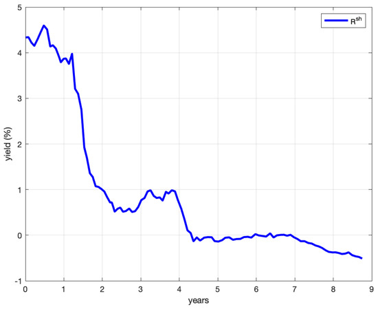
Figure 1.
The filter estimated value of the short−term interest rate .
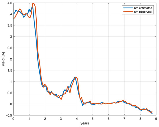
Figure 2.
Comparison between the market yield rate (blue line) and the model−implied yield rate (red line) for the 6-month maturity.
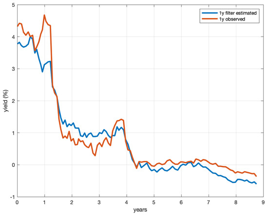
Figure 3.
Comparison between the market yield rate (blue line) and the model−implied yield rate (red line) for the 1−year maturity.
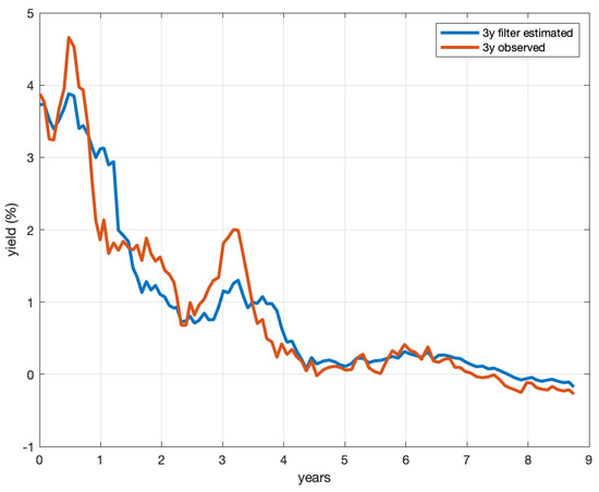
Figure 4.
Comparison between the market yield rate (blue line) and the model−implied yield rate (red line) for the 3−year maturity.
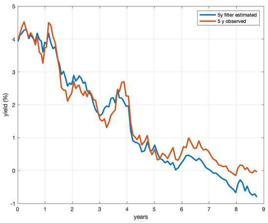
Figure 5.
Comparison between the market yield rate (blue line) and the model−implied yield rate (red line) for the 5−year maturity.
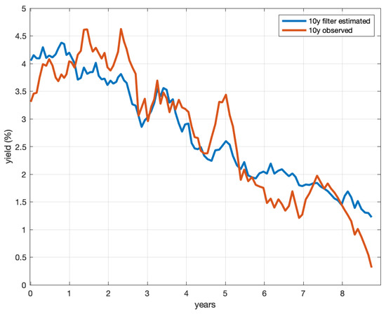
Figure 6.
Comparison between the market yield rate (blue line) and the model−implied yield rate (red line) for the 10−year maturity.
We used our model, with the parameters progressively calibrated as described in Section 4, to make an out-of-sample forecast. Figure 7 shows the predicted values for the 20-year maturity ZCB, computed using the short-term interest rate and the parameter values estimated by the maturities up to 10 years.
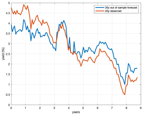
Figure 7.
Comparison between the market yield rate (blue line) and the model−implied yield rate (red line) for the 20−year maturity.
Table 1 reports, for each considered maturity, the root mean-squared error from March 2007 to October 2015 :

Table 1.
The root mean-squared error for each considered maturity. The last error is for the out-of-sample forecast of the 20-year yield.
From Figure 2, Figure 3, Figure 4, Figure 5, Figure 6 and Figure 7 and the error table, the curve of the model-implied ZCB yields appears to follow the Y curve of the market ZCB yields quite well. Even more significantly, Figure 7 shows that the model had a good predictive power for other bonds not included in the sample used for the calibration. The fit was even more meaningful as the ZCB yields underwent major changes in the period from March 2007 to December 2015. All these results confirmed that our model described the market evolution well.
Our model was not a “black box” one, but attempted to capture the interactions among inflation, the CB interest rate, and the short-term interest rate employing relatively few parameters. Table 2 reports the values of the parameters calibrated using the information for the first 100 months. In particular, the value confirmed that the interaction between the short-term interest rate and the CB interest rate cannot be neglected.
Table 2.
The estimated parameters.
We also conducted an ex post analysis of residuals. Precisely, for the dynamics of the inflation rate, we calculated the residuals , where and are the observed values of the inflation index and the CB rate, and was computed using the parameter values of Table 2. We applied the Jarque–Bera normality test: the normality null hypothesis could not be rejected, at a confidence level of 95%. The value of the statistics was , with a critical value of and a p-value of . Figure 8 shows a comparison between the empirical distribution function of the standardized residuals and the standard normal distribution function.
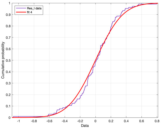
Figure 8.
The standard normal distribution (red line) and the empirical distribution (blue line) of the standardized residuals for inflation.
Here, the -norm of the difference was .
Similarly, we analyzed the residuals , computed using the parameter values of Table 2 and the value of provided by the filter. Under the Jarque–Bera test for both the five-year and ten-year bond yield, the null hypothesis of normality could not be rejected, at a confidence level of 95%. The value of the statistics was for the five-year bond and for the ten-year bond, with a p-value of . Figure 9 and Figure 10 show the plot of the empirical distribution of residuals for both maturities. The -norm of the difference between the empirical distribution function of the standardized residuals and the standard normal distribution function for both maturities was for the five-year bond and for the ten-year bond.
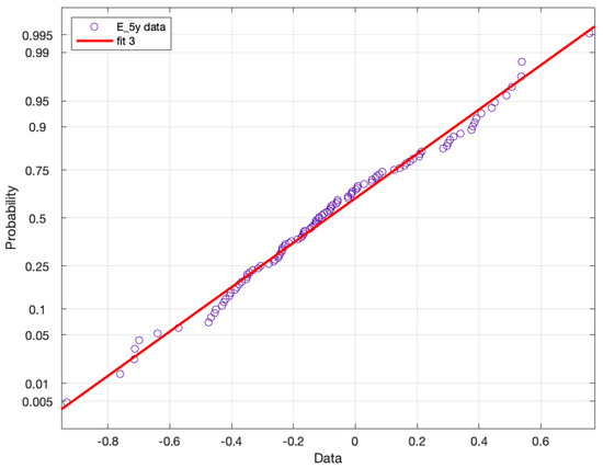
Figure 9.
Q-Q plot of the empirical distribution of the standardized residuals for the 5-year bond yield.
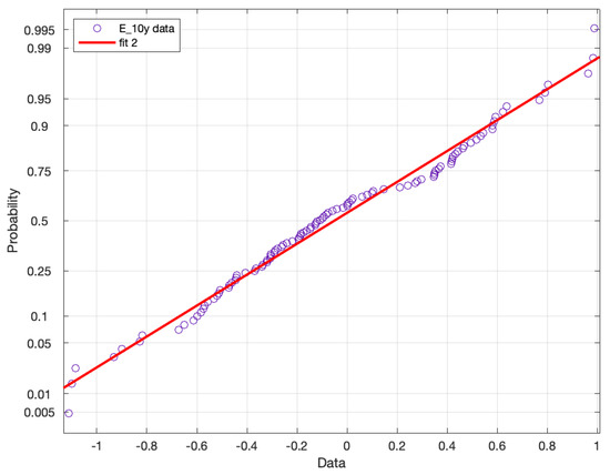
Figure 10.
Q-Q plot of the empirical distribution of the standardized residuals for the 10-year bond yield.
6. Conclusions
We considered the model that we proposed in a previous paper [21] to describe the joint evolution of inflation, the central bank interest rate, and the short-term interest rate. Our model involved only factors with a clear economic interpretation and employed far fewer parameters than the other ones known from the literature. We showed that, in the case when the diffusion coefficient did not depend on the CB interest rate, our model yielded a semi-closed valuation formula for contingent derivatives, in particular for ZCBs.
By using ZCB yields as observations, we implemented the Kalman filter and obtained a dynamical estimate of the short-term interest rate . By employing again our valuation formula, this estimate provided a one-step-ahead prediction of the ZCB yields. By using this prediction, at each time step, we made a quasi-maximum likelihood estimation of the model parameters under the risk-neutral measure and of the coefficient of the risk premium. Considering the values of the parameters calibrated using the information from the first 100 months, we saw that the value confirmed that the interaction between the short-term interest rate and the CB interest rate cannot be neglected.
We compared the market values of German ZCB yields for several maturities with the corresponding values predicted by our model, from 2007 to 2015. The model-implied values followed the market values quite closely, even though the ZCB yields underwent major changes during the considered period. Even more significantly, our model and the filtering/calibration procedure provided quite a good prediction for the 20-year ZCB yield, which was not included in the sample used to estimate the values of the short-term interest rate and of the parameters.
The main limitation of the estimation procedure we proposed was that it required numerically computing some of the quantities involved in the valuation formula. One of the directions of research that we intend to pursue in the near future is looking for faster numerical methods, for instance by using the fast Fourier transform. We also intend to look for special cases in which a closed valuation formula is available.
However, our procedure was already fast enough that it can be applied by practitioners to estimate the short-term interest rate and compute its one-step-ahead prediction, as well as to use them in pricing derivatives. Note that our model also allowed pricing inflation-linked derivatives (see [21]).
Finally, other near-future research projects of ours are using our model to evaluate more sophisticated fixed-income derivative instruments, for example credit risk derivatives, and to embed parts of our model in a model where the CB interest rate is viewed as part of a strategy of the monetary policy decision maker.
Author Contributions
Conceptualization, F.A., C.C. and M.P.; investigation, F.A., C.C. and M.P.; methodology, F.A., C.C. and M.P.; writing—original draft, F.A., C.C. and M.P.; writing—review and editing, F.A., C.C. and M.P. All authors read and agreed to the published version of the manuscript.
Funding
This research received no external funding.
Institutional Review Board Statement
Not applicable.
Informed Consent Statement
Not applicable.
Data Availability Statement
Not applicable.
Acknowledgments
We are grateful to two anonymous reviewers for their helpful comments.
Conflicts of Interest
The authors declare no conflict of interest.
Appendix A
In (40), in order to compute , we have to compute , , by using (26), with , and by numerically solving the system (27)–(29) with and . In this Appendix A, we describe the numerical procedure that we set up to do this. In the sequel, we omitted the subscript j and wrote for . Taking into account that , if , , , this amounts to solving, for each :
- for ,with terminal condition:
- for ,with terminal condition:where denotes the Gaussian density of zero mean and variance ;
- for ,with terminal condition:
Then:
From now on, we considered only the equation for : the computations for and are completely analogous. In addition, we omitted the subscript 0.
We considered values of r in the discrete, increasing set , where , , and . Setting , we obtained, for each , the following system of backward ordinary differential equations:
By inverting the time direction and defining as the vector of components , the above system of ordinary differential equations can be rewritten as:
where:
The initial datum is:
It would be natural to approximate the integral in (A3) by a sum of the form:
where is the discretization step for the variable u. To this end, for each and k, we would need to compute the value of on the D points , which in turn would require computing the value of on the points , …, , …, , …, , and so on, so that, for each pair , we would need to compute on a grid of points and a different one for each .
In order to simplify the computation, we defined, for each , independently of k, a sequence of grids , …, constructed in the following way:
where we considered, for numerical purposes, only values , , and , . , , , and are the parameters in , and is the interval in which the variable r takes values (, ). Taking into account that , for all ,
so that for each , there is an index such that:
Then, we can replace by a linear interpolation between and . This procedure is repeated up to L. In this way, at step j, we needed to compute only on the level j grid points. As the number of the grid points increases linearly in j, the total number of points in all grids is of the order of . Finally, we solved the system—(A1) and (A2) by a standard routine.
References
- Cox, J.C.; Ingersoll, J.E., Jr.; Ross, S.A. A theory of the term structure of interest rates. Econometrica 1985, 53, 385–408. [Google Scholar] [CrossRef]
- Akram, T.; Li, H. An inquiry concerning long-term US interest rates using monthly data. Appl. Econ. 2020, 52, 2594–2621. [Google Scholar] [CrossRef]
- Jarrow, R.; Yildirim, Y. Pricing treasury inflation protected securities and related derivatives using hjm model. J. Financ. Quant. Anal. 2003, 38, 409–430. [Google Scholar] [CrossRef]
- Singor, S.N.; Grzelak, L.A.; Van Bragt, D.D.B.; Oosterlee, C.W. Pricing inflation products with stochastic volatility and stochastic interest rates. Insur. Math. Econ. 2013, 52, 286–299. [Google Scholar] [CrossRef]
- D’Amico, S.; Kim, D.H.; Wei, M. Tips from TIPS: The Informational Content of Treasury Inflation-Protected Security Prices; Working Paper; U.S. Federal Reserve Board: 2009. Available online: https://www.bis.org/publ/work248.htm (accessed on 26 April 2021).
- D’Amico, S.; Kim, D.H.; Wei, M. Tips from TIPS: The Informational Content of Treasury Inflation-Protected Security Prices. J. Financ. Quant. Anal. 2018, 53, 395–436. [Google Scholar] [CrossRef]
- Ho, H.W.; Huang, H.H.; Yildirim, Y. Affine model of inflation-indexed derivatives and inflation risk premium. Eur. J. Oper. Res. 2014, 235, 159–169. [Google Scholar] [CrossRef]
- Waldenberger, S. The affine inflation market models. Appl. Math. Financ. 2017, 24, 281–301. [Google Scholar] [CrossRef]
- Hughston, L.P.; Macrina, A. Information, Inflation and Interest, Advances in Mathematics of Finance; Banach Center Publications, Institute of Mathematics Polish Academy of Sciences: Warszawa, Poland, 2008. [Google Scholar]
- Haubric, J.; Pennacchi, G.; Ritchken, P. Expectations, Real Rates, and Risk Premia: Evidence from Inflation Swaps. Rev. Financ. Stud. 2012, 25, 1588–1629. [Google Scholar] [CrossRef]
- Duran, M.; EGulsen, E. Estimating inflation compensation for turkey using yield curves. Econ. Model. 2013, 32, 592–601. [Google Scholar] [CrossRef]
- Grishchenko, O.V.; Vanden, J.M.; Zhang, J. The informational content of the embedded deflation option in TIPS. J. Bank Financ. 2016, 65, 1–26. [Google Scholar] [CrossRef][Green Version]
- Hinnerich, M. Inflation-indexed swaps and swaptions. J. Bank Financ. 2008, 32, 2293–2306. [Google Scholar] [CrossRef]
- Belgrade, N.; Benhamou, E.; Koehler, E. A Market Model for Inflation. 2004. Available online: https://ssrn.com/abstract=576081 (accessed on 26 April 2021).
- Brody, D.; Crosby, J.; Li, H. Convexity Adjustments in Inflation-Linked Derivatives. 2008. Available online: https://www.risk.net/derivatives/inflation-derivatives/1500259/convexity-adjustments-inflation-linked-derivatives (accessed on 26 April 2021).
- Stewart, A. Pricing Inflation-Indexed Derivatives Using the Extended Vasicek Model of Hull and White. Master’s Thesis, University of Oxford, Oxford, UK, 2007. [Google Scholar]
- Dodgson, M.; Kainth, D. Inflation-Linked Derivatives; Royal Bank of Scotland Risk Training Course; Market Risk Group: 2006. Available online: http://citeseerx.ist.psu.edu/viewdoc/download?doi=10.1.1.623.9549&rep=rep1&type=pdf (accessed on 4 April 2021).
- Eksi, Z.; Filipovic, D. Pricing and hedging of inflation-indexed bonds in an affine framework. J. Comput. Appl. Math. 2014, 259, 452–463. [Google Scholar] [CrossRef]
- Vig, A.A.; Vidovics-Dancs, A. Indexed bonds with mean-reverting risk factors. In Proceedings of the 31st European Conference on Modelling and Simulation, Budapest, Hungary, 23–26 May 2017. [Google Scholar]
- Chuang, M.C.; Lin, S.K.; Chiang, M.H. Pricing the Deflation Protection Option in TIPS Using an HJM Model with Inflation-and Interest-Rate Jumps. J. Deriv. 2018, 26, 50–69. [Google Scholar] [CrossRef]
- Antonacci, F.; Costantini, C.; D’Ippoliti, F.; Papi, M. Inflation, ECB and short-term interest rates: A new model, with calibration to market data. arXiv 2020, arXiv:2010.05462. [Google Scholar]
- Costantini, C.; Papi, M.; D’Ippoliti, F. Singular risk-neutral valuation equations. Financ. Stoch. 2012, 16, 249–274. [Google Scholar] [CrossRef]
- Babss, S.H.; Nowman, K.B. Kalman Filtering of Generalised Vasicek Term Structure Models. J. Financ. Quant. Anal. 1999, 34, 115–130. [Google Scholar] [CrossRef]
- Chatterjee, S. Application of the Kalman Filter for Estimating Continuous Time Term Structure Models: The Case of UK and Germany; Working Paper; Business School, University of Glasgow: Glasgow, UK, 2005. [Google Scholar]
- Chen, R.R.; Scott, L. Multi-factor Cox-Ingersoll-Ross models of the term structure: Estimates and tests from a Kalman filter model. J. Real Estate Financ. Econ. 2003, 27, 143–172. [Google Scholar] [CrossRef]
- Vo, L.H. Application of Kalman filter on modeling interest rates. J. Manag. Sci. 2014, 1, 1–15. [Google Scholar]
- Christoffersen, P.; Dorion, C.; Jacobs, K.; Karoui, L. Nonlinear Kalman Filtering in Affine Term Structure Models. Manag. Sci. 2014, 60, 2248–2268. [Google Scholar] [CrossRef]
- Jacod, J.; Shiryaev, A.N. Limit Theorems for Stochastic Processes, 2nd ed.; Springer: Berlin/Heidelberg, Germany, 2003. [Google Scholar]


Publisher’s Note: MDPI stays neutral with regard to jurisdictional claims in published maps and institutional affiliations. |
© 2021 by the authors. Licensee MDPI, Basel, Switzerland. This article is an open access article distributed under the terms and conditions of the Creative Commons Attribution (CC BY) license (https://creativecommons.org/licenses/by/4.0/).