1. Introduction
The theory of thermoelasticity has received a lot of interest from researchers and scientists due to its many applications in different fields. The fields of architecture, structural features, plasma physics, geophysics, aeronautics, missiles, steam turbine generators, etc. are among the most important areas in which this theory is used. For the first time, an uncombined principle of thermoelasticity was foreseen, in that the elastic strain is independent of the heat transfer and conversely. However, this hypothesis became invalid in displaying the practical results of many concrete problems. Then, researchers provided alternative theories of coupled thermoelasticity, which became widely known as a general thermoelastic theory. This concept has been gaining fame in recent years because its aim is to solve the contradiction of the unlimited heat propagation rate. This description, however, has become appropriate to some extent to communicate practical performance, such as high-speed energy transportation and low-temperature and high-heat transfer engineering.
The classical coupled thermoelasticity theory (CTE) [
1] suggested by Biot expects a theoretically unrealistic unlimited velocity of the spread of heat. In order to remove the contradiction of the extraordinary physical phenomenon of unlimited speed in the CTE theory, non-classical thermoelasticity models known as generalized thermoelasticity have been formulated. Lord–Shulman [
2], Green–Lindsay [
3], and Green–Naghdi [
4,
5,
6] theories are major theories of generalized thermoelasticity that became the focus of current research in this field. Lord and Shulman [
3] integrated the principle of heat flow rate into the law of Fourier with thermal relaxation time, and formulated a theory of extended thermoelasticity with a thermal flux rate. The energy equation as well as the relationship between Duhamel and Neumann were altered by Green and Lindsay [
4], providing two relaxation periods. Theories of thermoelasticity without and with energy dissipation [
4,
5,
6] have been proposed by Green and Naghdi. Roychoudhuri [
7] suggested the three-phase-lag (TPL) thermoelastic model that involves three different phase delays in the heat flux vector, the gradient of temperature, and the gradient of thermal displacement function. The prevalent problems of thermoelasticity based on these new models are now of great significance [
8,
9,
10,
11,
12,
13].
The Moore–Gibson–Thompson Equation (MGT) has been heavily involved in a broad range of papers focused on study and understanding in recent decades. This concept stems from a differential equation of the third order, which is involved in the value of several dynamic fluid aspects [
14]. Quintanilla [
15] has built a new model of thermo-elastic heat conduction (called “MGT thermoelasticity”) based on the Moore–Gibson–Thompson equation. Another new thermoelastic model with two temperatures, in which heat conduction was described as the historical MGT version, was given by Quintanilla [
16], which emerged from the development of the theory of Green–Naghdi Type III by adding a relaxation factor. In the context of several mechanical aspects of the flux, this theory started with a third-order differential equation. The MGT thermoelastic model has led to a significant increase in the range of researchers devoted to this theory [
17,
18,
19,
20,
21,
22,
23,
24,
25,
26,
27,
28,
29,
30].
Diffusion is the transition from a higher concentration area to a less centered region (such as molecules, atoms, and ions). A mathematical relationship dependent on the concentration gradient defines diffusion. This phenomenon has resulted in several industrial purposes from the recent interest. In many fields, the diffusion concept is commonly used, including physics, economics, biology, sociology, chemistry, and finance. In bipolar transistor diffusion, integrated resistors are formed to form a base and emitter; spring/drain regions are formed in the MOS transistor, and dopes are formed in the MOS gated polysilicon transistor. Concentration is determined by what is called Fick’s Law in many of these areas of application. This is a basic law that does not deal with the interactions between the input substance and the medium in which the substance is incorporated or the effect of temperature on this reaction [
31,
32,
33].
One of the distinguishing features of diffusion is that it depends on the spontaneous movement of particles, which, without the need for a direct mass movement, leads to mixing or mass transfer. One of the elements of approximation, or collective action, is a mass movement. The term “convection” describes the combination of two phenomena of transport. Temperature, contact zone, gradient steepness of concentration, and particle-size-effect diffusion. The rate and degree of diffusion can be adjusted independently and collectively by each factor. Entropy inequality is suggested for the blend and is used to restrict the constituent equations in a mixture of elastic materials subject to diffusion and thermal management. The constituents are later assumed to be isotropic solids and further restricted to the material frame–differentiation axiom and to reflect symmetrical conditions of the material. It is shown that the constituent functions can be written with respect to the left Cauchy–Green tensors for constituents.
Thermo-diffusion in solids, particularly metals, has been regarded as an unrelated amount of body deformation until recent times. Even so, a study demonstrates that the thermo-diffusing process can have a major impact on body deformation. The Thermoelastic diffusion concept was introduced by Nowacki [
33,
34,
35]. The developed thermoelastic model was proposed in this concept. This requires propagation at infinite rates of thermoelastic waves. Sherief et al. [
36] established a thermoelastic generalization theory suggesting limited spreading velocities for thermoelastic and propagating waves. In terms of the principle of generalized thermoelastic diffusion, Sherief and Saleh [
37] and Sherief and Maghraby [
38] have worked on a thermoelastic half-space issue with a permeating substance in contact with the bonding surface.
The thermo-diffusion theory and the combination of quasi-stationary diffusion problems for an elastic substrate have been investigated by several researchers [
32,
39,
40,
41,
42,
43,
44]. The effects of cross-effects caused by the mixture of temperature, mass diffusion, and strain were studied, resulting in additional mass concentration due to thermal excitation and producing additional temperature ranges [
45,
46,
47,
48,
49,
50].
It was found from previous studies that the theory of the third form (GN-III) by Green and Naghdi has a similar defect as the usual Fourier model and also forecasts the immediate spread of thermal waves. Giorgi et al. [
45] explained that such phenomena relevant to constant states are outside the control of the theory of Type III, which should be seen in Fourier as a principle of thermal conduction rather than as a simple theory. This theory is true for both stationary and sluggish thermal phenomena. To solve this dilemma, it is, therefore, natural to amend this suggestion. A new theory of thermal diffusion is formulated in this present work, in which the Moore–Gibson–Thompson equation defines the heat conduction and diffusion formulae. This model was designed to explore the interaction between elasticity, heat, and the mechanisms of diffusion of elastic materials that allow the propagation of thermal waves at finite rates. Many studies have been performed on the inversion of the Laplace transform in the literature [
51,
52,
53,
54,
55,
56,
57,
58]. More details for them will be given in the next sections. Indeed, the governing system equations can be realized in the new model after the addition of two relaxation factors in the GN-III model. Discrete singular convolution is also applied for some heat and cavity problems [
59,
60]. A modified and correct solution technique is proposed using the integral boundary formulations of the heat equation by Chernov and Reinarz [
61].
The topic of thermo-diffusion interactions in an unbounded isotropic homogeneous solid with a cylindrical hole has been researched in the sense of the generalized model of Moore–Gibson–Thompson thermo-diffusion (MGT-TD). The surface of the cylinder is free of traction and, respectively, undergoes time-dependent convection and chemical load. By means of the Laplace transform method, an accurate solution to the issue is obtained first. The Laplace transformations have been reversed numerically. To show the diffusion effects and different physical phenomena of these solids, the study findings have also been numerically measured and graphically portrayed. Numerical values have been provided in figures and tables to illustrate the comparisons between the physical fields in order to allow a distinction between the results we obtained and the corresponding results in other special models.
2. The Basic MGT Thermo-Diffusion Equations
Many mathematicians, physicists, and engineers, as well as industry, widely use Fourier and Vic formulas to explain the thermal conductivity and diffusion in elastic materials. In this section, we will derive a new paradigm that allows describing the phenomena of heat transfer as well as propagation within materials in a manner consistent with the physical and chemical aspects.
In a homogeneous isotropic, elastic solids, the governing equations, and constitutive relationships for generalized thermo-diffusion behavior are established by [
33,
34,
35]. The Fourier’s law:
The strain–displacement relations:
The coupled conservation heat energy equation:
The continuity equation [
46]:
The chemical potential
:
where heat flux
,
denotes the temperature increment in which
is the absolute temperature,
is the reference temperature,
indicates the thermal conductivity,
denotes the strain tensor and
is the displacement vector. Additionally, in Equations (1)–(6),
denotes the chemical potential,
denotes the flow of the diffusing mass vector,
is the diffusion coefficient, where
is the cubical dilatation,
is the source of heat,
is the density of the medium,
denotes the specific heat at constant strain,
is the measure of thermoelastic diffusion effect,
is the concentration of the diffusive material and
are the material constants (thermoelastic coupling), where
is the coefficient of the thermal expansion.
Although the elastic thermal diffusion laws of Fourier and Fick have been well tested for most practical problems, they do not specify a temporary short-time temperature area (higher frequencies and smaller wavelengths). We obtain parabolic partial differential equations through the combination of Equation (1) with (4) and (2) with (5). They emit an infinite velocity of propagation as a result. This property, from a physical point of view, conflicts with physical phenomena. In the past 3 decades, the non-classical diffusion and thermal elasticity theories have been replaced by more general equations to solve the previous inconsistency issue. The generalized model of thermo-diffusion with a time of relaxation was developed by Sherief et al. [
36], which allows thermal wave propagation to be reduced.
In 1948, to solve the infinitely rapid propagation in the heat equation, Cattaneo proposed an updated equation for the heat equation. The relationship (1) was replaced by
where
is a thermal relaxation time parameter. Sherief et al. [
36] postulated a similar mass flow equation in the same way and similar to Equation (7), given by:
where
indicates the diffusion time relaxation parameter. This ensures that the
equation also forecasts the limited velocity of spread of the substance from medium to media. This is achieved with concentration
.
The development of an alternative construction of heat diffusion was then suggested by Green and Naghdi [
4,
5,
6] as an entirely new thermoelastic theory. The function
is seen as a new constituent vector in the models of Green and Naghdi as a gradient of thermal displacement. In mechanical fields and in thermal fields, the scalar function
is generally seen as the mechanical displacement equivalent. In addition, the function
fulfills
. The law of improved thermal conductivity of the GN-III theory is described as [
5]
In this instance, the parameter
is a constant material property and is also mentioned as the heat conductivity rate. Abouelregal [
39,
40] suggested a similar relation for the vector of heat flow to Equation (9) as:
In Equation (10), the chemical displacement rate is regarded as a new constitutive variable in which parameter is the diffusion rate factor. The chemical displacement function satisfies the relation .
The combination of Fourier’s modified law (9) and energy Equation (4) has been found to lead to a series of elements in the point continuum, rendering the actual component infinitely dependent on the solutions. Equation (9) has the exact same flaw as the usual Fourier hypothesis that the waves of thermal conduction spread instantly. Therefore, this proposal was also generally updated, and Quintanilla [
15,
16] included a relaxation time to solve this problem, given the MGT equation. Quintanilla [
15] made an adjustment to the proposed updated heat conduction equation (MGTE) after adding the relaxation factor in the Green–Naghdi form III model as follows:
By differentiating Equation (11) and using the relationship
, we have
As in Equation (11), the mass flux Equation (10) is assumed to be similar:
After differentiating the previous relationship with respect to time and using
, we obtain
By combining Equations (4) and (12), a modified type of heat conduction equation can be obtained, which is developed based on the MGTE equation [
15,
16]. When we take a divergence operator to Equation (12) and use Equation (4), we obtain:
We also obtain the modified equation of mass diffusion by taking the divergence of Equation (15) and the use of Equations (5) and (6) as
Complementing the system of equations that govern the behavior of thermal, dynamic, and diffusion propagation inside bodies with normal properties and homogeneity, we have [
36]:
where and
is a material constant (diffusion coupling) given by
, where
is the coefficient of the linear diffusion equation,
is the stress tensor,
and
are Lame’s constants, and
is the Kronecker delta function.
Equation (15) occurs in viscous thermal soothing applications, with high intensity, medical and industrial applications such as lituosis, thermal therapy, or ultrasound washing. The model is also known as the Kelvin or Zener model. This equation is found in the viscoelasticity theory, the classic linear viscoelastic model, to clarify the conduct of certain viscoelastic materials, including the complex and viscous micro-structures of fluids [
48].
5. Solution in the Laplace Transform Domain
Applying the Laplace transform to Equations (31)–(36) under the initial conditions (38), described by
we obtain
where
Eliminating
,
between Equations (43)–(45), we obtain
where
By the same manner, we can demonstrate that the functions
and
can fulfill the equations
Introducing the parameters
(
into Equation (50), we have
where
and
are the solutions for the equation:
The parameters
,
and
can be determined as
The solution of Equation (54), which is infinitely limited, is given by
where
are the integral parameters and
denotes the second kind of Modified Bessel function of zero order. Likewise, we can write
Inserting Equations (58) and (59) into Equations (43)–(45), the following relations can be obtained
Then, Equations (58) and (59) may be expressed as
After using the relationship between
and
, the solution of the radial displacement
will be
Using the expressions (57), (61)–(63) and the well-known relation
we can obtain the solutions of the thermal stresses and the chemical potential as
The boundary conditions in Equations (39)–(41) at
in the transformed domain may be expressed as
Using the boundary conditions (68) with Equations (57), (65), and (67), the following linear system of equations can be obtained:
The unknown parameters , and can be determined by resolving the system (69)–(71). By the setting of the constants , and and substitution in the general solutions of the different functions, this means that we have finished solving the problem in the field of the Laplace Transform.
5.1. Generalized MGT Model of Thermoelasticity without DIFFUSION
In this case, we take
. However, the functions
and
may be obtained Laplace transform domain by solving the two differential equations:
Eliminating
or
in the above equation, one obtains the fourth-order differential equation:
where
The solutions to Equation (55) are given by
where
,
(
) are integral constants and
are given by
Based on these solutions, the quantities of other physical fields can be simplified in the same way as in the previous analysis:
To complete the solution in this case, the boundary conditions in Equations (39) and (40) are sufficient to obtain the integral constants ().
5.2. Special Cases of Thermoelasticity and Thermo-Diffusion Models
The model and equations derived and obtained in the second section of this paper are valid for many special cases that can be inferred from our constructed model. A system of equations containing thermal conduction equation (Equation (15)) and diffusion equation (Equation (16)) may include at least 10 generalized theories of thermal elasticity in the absence of diffusion as well as some generalized diffusion theories. The following can be summarized and documented in some special cases:
Case I: When the diffusion effect is absent
If the diffusion effect is missing (), it is possible to obtain the following models:
The traditional theory of thermoelasticity (CTE) [
1] when
.
The Lord and Shulman generalized theory (LS) [
2] by setting
.
The Green and Naghdi model of Type II (GN-II) [
6] when the first term on the right-hand side of Equation (15) is disregarded and
.
The Green and Naghdi theory of Type III (GN-III) [
5] when
.
The Moore–Gibson–Thompson thermoelasticity theory MGTE [
15,
17] when
.
Case II: Taking into account the effect of diffusion
5.3. Inversion of the Laplace Transforms
Many problems have solutions that may be expressed in terms of a Laplace transform, which is therefore too difficult to invert using complex analysis techniques. The numerical evaluation of the Laplace inversion integral has been accomplished using a variety of approaches. Many papers have been written in the literature on the inversion of the Laplace transform. See, for example, [
51,
52,
53,
54], and a detailed bibliography can be found in [
55,
56].
Some methods work amazingly well with some image functions, while providing horrific results for others. Since no approach is best in all cases, we recommend using several alternative strategies to solve a particular reversal problem. We can be more confident and accept a numerically inverse Laplace transform if two or more methods give approximately the same result. In [
57], Abate and Valkó have classified those algorithms into four categories according to the basic approach of the method as follows: (1) Fourier series expansion; (2) Laguerre function expansion; (3) combination of Gaver functionals; (4) deform the Bromwich contour.
This work presents the numerical inversion technique of Laplace transforms based on the Durbin and Fourier series expansion [
58] and Honig and Hirdes [
53]. The disadvantage of this type of inversion method, the remarkable dependence of estimation, and truncation error on free parameters is overcome by applying a procedure to reduce the estimation error, a method to speed up the Fourier series convergence, and a procedure that roughly computes the “best” option for all free parameters at the same time. For two reasons, this approach is effective in meeting the demands of standalone digital computing. Compared to other more complex numerical squaring methods, it is fast (economical) on the digital computers that are currently accessible. Second, because the inverse function is given as a Fourier cosine series with the coefficients being acceptable forward transform values, the technique is theoretically straightforward and requires minimal programming effort.
The Laplace transform and its inversion formula of the function
f(
t) are defined as follows:
where
is arbitrary but must be chosen so that it is greater than the real parts of all the singularities of
. For purposes of discussion, it is herein assumed that these integrals exist for
. Using the inversion formula
which is equivalent to (2) with
,
, and a Fourier series expansion of
in the interval
, Durbin derived the approximation formula
where the parameter
is a satisfactorily large integer and denotes the number of stops in the truncated Fourier series. The parameter
can be chosen so that it is
where
is a persecuted small positive number that corresponds to the degree of accuracy to be achieved. A good choice of free parameters
and
is important not only for the accuracy of the results but also for the application of the “Korrektur” method and convergence acceleration methods. These methods do not improve results if the parameters are badly chosen. For faster convergence, numerical experiments have shown that the value of the parameter
that satisfies the above relation is given in terms of time as
[
13].
6. Numerical Example and Discussion
We will now present some empirical results numerically to explain the new model introduced in this work and on the basis of preceding section outcomes. In order to answer the issue more comprehensively and to see how the studied fields depend on diffusion and certain physical influences, we have also numerically calculated for a particular physical material. The physical values of copper were selected for the purpose of mathematical estimation. The properties of this substance are therefore given in the SI units as follows [
39,
40]:
All of the parameters calculated , and will be used in calculations unless are determined otherwise. The numerical procedure defined in (84) has been applied to obtain the temperature , displacement , radial stress , hoop stress , and concentration as the chemical potential distributions within the medium. We assume that the cylinder cavity, with its center, has a radius of from the origin.
By comparing the basic Green and Naghdi theories of the second and third types with the modified thermal diffusion model, this section will provide some examples and applications for testing the validity of the given model. Plot activities are seen in the hollows cylinder’s radial pathway. The tabulation of some of the results for future comparisons to other researchers is an important part of this study.
The effects of the field variables analyzed based on the thermo-diffusion theories CTED, CTED, GND-II, GND-III, and MGTED have been reported in Tables 1–6. In the radial direction of the cylinder, Figures 1–6 display further sample graphs of all models to assess the effect of various thermal diffusion models on the quantities of the physical fields.
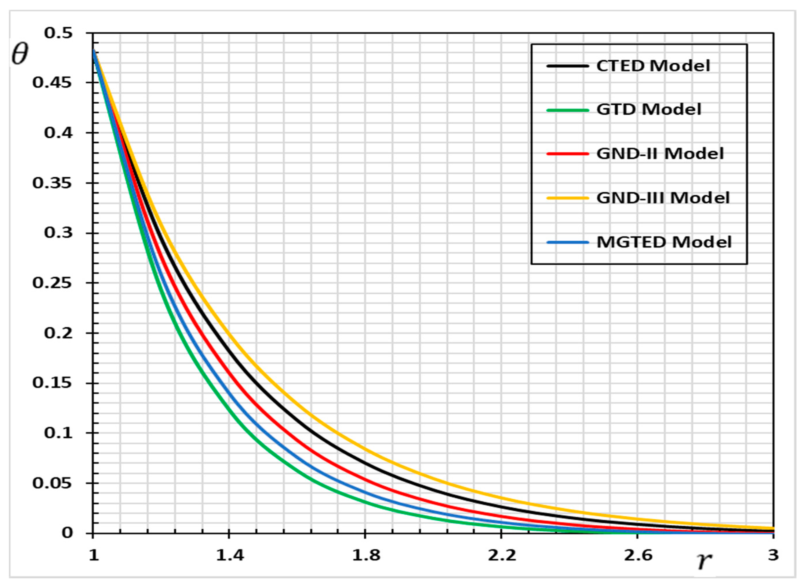
In the presence of the diffusion effect,
Table 1 and
Figure 1 display the variance of the temperature vs. the radial distance
for the different theories. The temperature values
reach the maximum values on the surface of the spherical cavity
as shown in the table and the figure, and then gradually decrease. The distribution of temperature satisfies the condition of the thermal boundary imposed upon the problem. The values of
gradually decrease and ultimately decrease in the opposite direction of the heat-wave propagation to a value of zero as the radius
increases.
A great difference in the temperature field has been found near the boundary surface of the body under all thermo-diffusion theories, considering the convergence of all models when increasing the radius within the body. It was also noted that in the CTED and GND-III models, higher temperature values were observed compared to the GN-II, GTD, and MGTED models. In the CTED and GND-III models, thermal waves do not fade easily, unlike in other thermal diffusion models in which it is clear that thermal waves spread at slow speeds inside the medium. This is because the heat waves in the CTED model propagate at an unlimited velocity. It is also noted that in the case of the MGTED model, the numerical values are lower inside the body away from the spherical cavity of the surface than in the case of the GND-III model, and the waves also fade away faster. The explanation for the rapid decrease, as predicted, is the inclusion of relaxation times in the equations extracted.
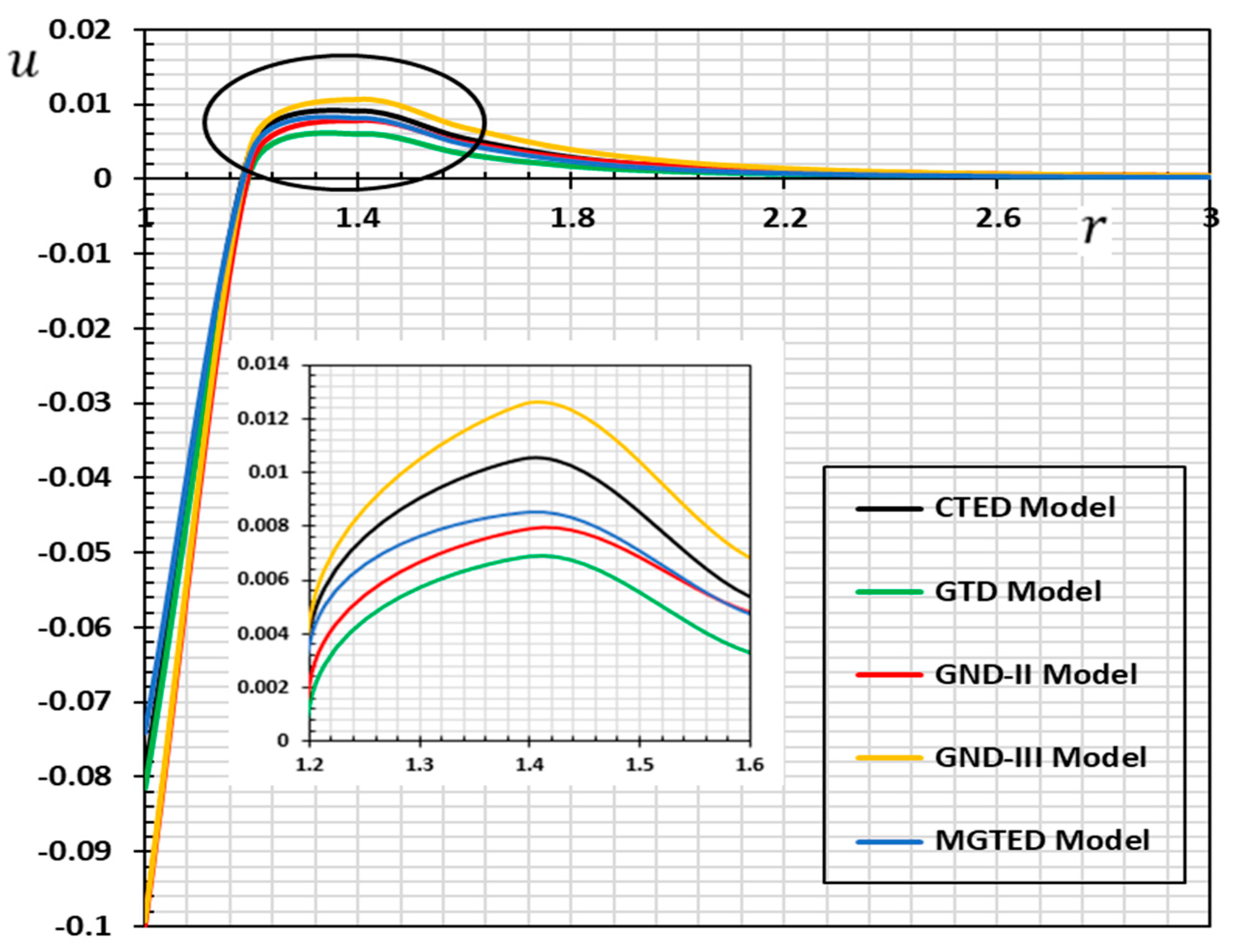
The effect of all thermal diffusion models on the displacement
in the radial direction of the cylinder is shown in
Table 2 and
Figure 2. The displacement distribution begins at a negative value and then increases gradually as the distance increases until it reaches a peak value of approximately
, after which it eventually decreases to zero with
increasing. From the table and figure, it can be seen that the relaxation times
and
that were used in the current thermo-diffusion model have a significant role to play in body deformation.
In the case of modified GTD, GND-II, and modified MGTED models, numerical values of disolactivity are also smaller compared to the findings of the CTED and GN-III models. In general, it seems that in various theories, there is great similarity and convergence in the action of displacement. Only in magnitude and peak points does the difference arise. It can be detected that when relaxation times are used, the displacement profile for the Green and Naghdi thermo-diffusion model (GND-III) is greater in the absence of relaxation times than for the MGTED thermo-diffusion model.
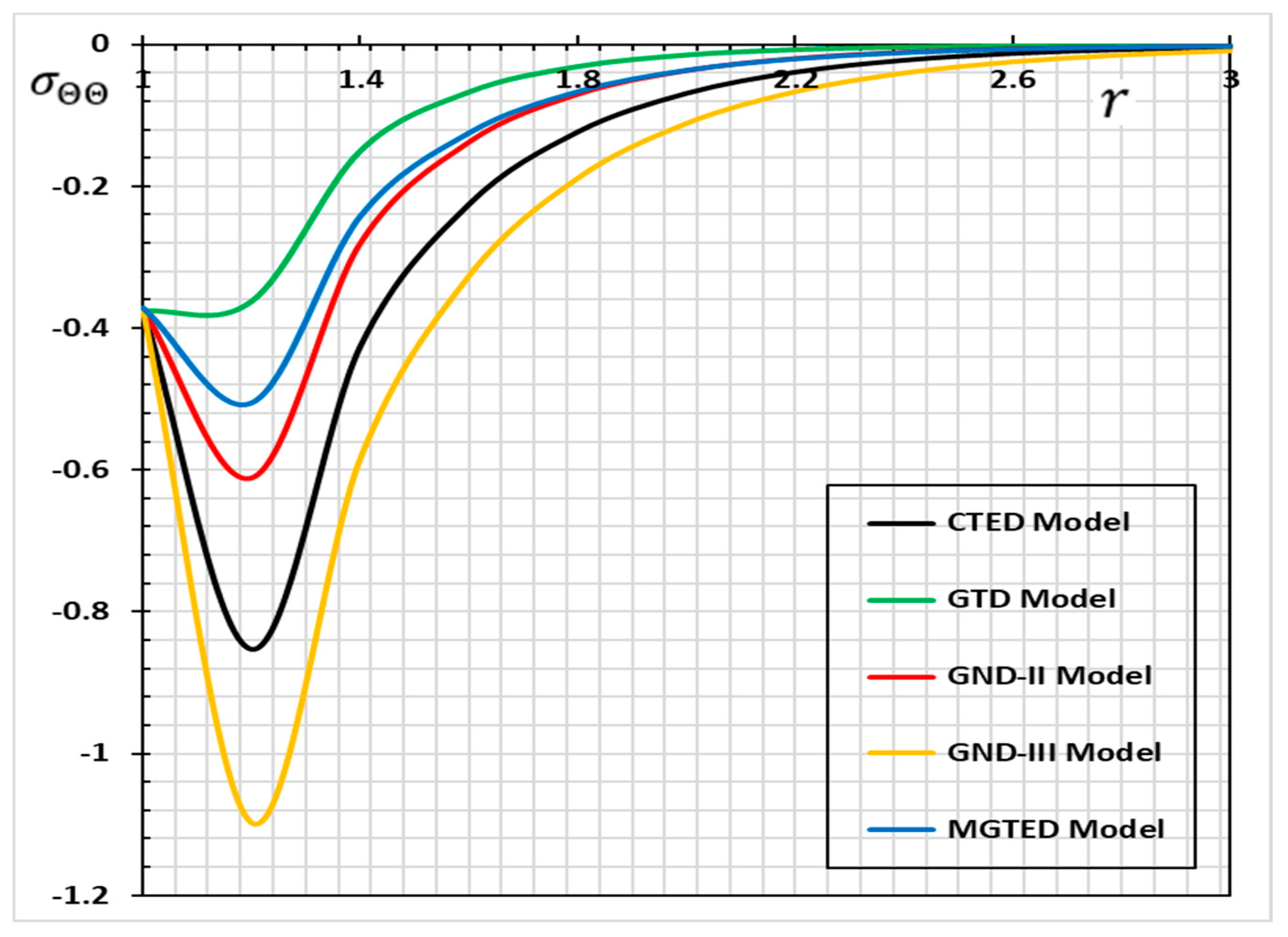
For various combinations of thermo-diffusion models,
Table 3 and
Table 4 and
Figure 3 and
Figure 4 are provided to investigate the effect of thermo-diffusion on the variance of thermal stresses
and
. The comparison between the various models and the various distributions of heat stress can be observed. It is also noted that, in comparison to the CTED model, the magnitudes of stress values in the case of thermal diffusion GN-III models are the largest possible.
The radial thermal stress
starts at zero, filling the conditions of the proposed problem, then decreases rapidly until at the peak point it reaches its maximum value, and then decreases steadily until it disappears to zero (see
Table 3 and
Figure 3). With the hoop stress
, the same previous behavior occurs except that it starts with a negative value different from zero at the surface of the spherical cavity. In behavior and principles, the variations in GTD-, GND-II-, and MGTED-generalized thermal diffusion models are similar together.
The existence of the relaxation parameters of generalized thermoelasticity (GND-III) and the diffusion that have been integrated into the current model (MGTED) have a major effect on the properties and actions of the vibrations of the different distributions.
It can be attributed to the compressive essence of stress that atoms are suppressed together in the solids and voluminously induce compressive stress because of the dissolution of the substance. In both cases, the comparison of each figure shows that, as time pass away from the source, the magnitude of the various quantities considered decreases, thus showing the wave fronts.
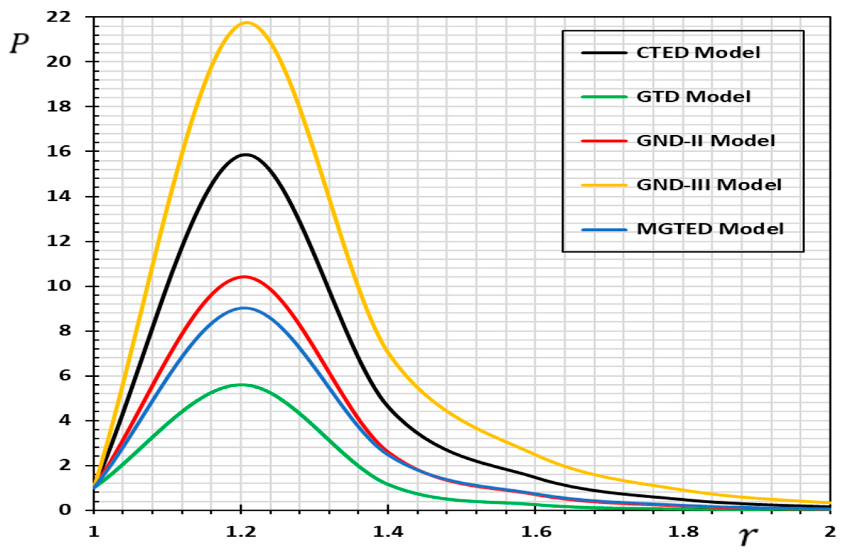
For the five separate thermo-diffusion models, the numerical computations of the chemical potential
against the radial distance
are shown graphically in
Figure 5 and in
Table 5.
Figure 5 and
Table 5 show that at the beginning, the variance of the chemical potential
is great and that the vibrations of the transition decrease and fade as the
value increases. The chemical potential
profile has also been established, starting with the greatest surface value, meeting the boundary conditions imposed on the problem, and this confirms and validates the outcomes we have obtained. In
Figure 5 and
Table 5, we note that the variations in the case of CEDT and GND-III are similar to each other and have the highest values, while the GTD models GND-II and MGTED are smaller in size due to the effect of generalized thermal and diffusion relaxation parameters.
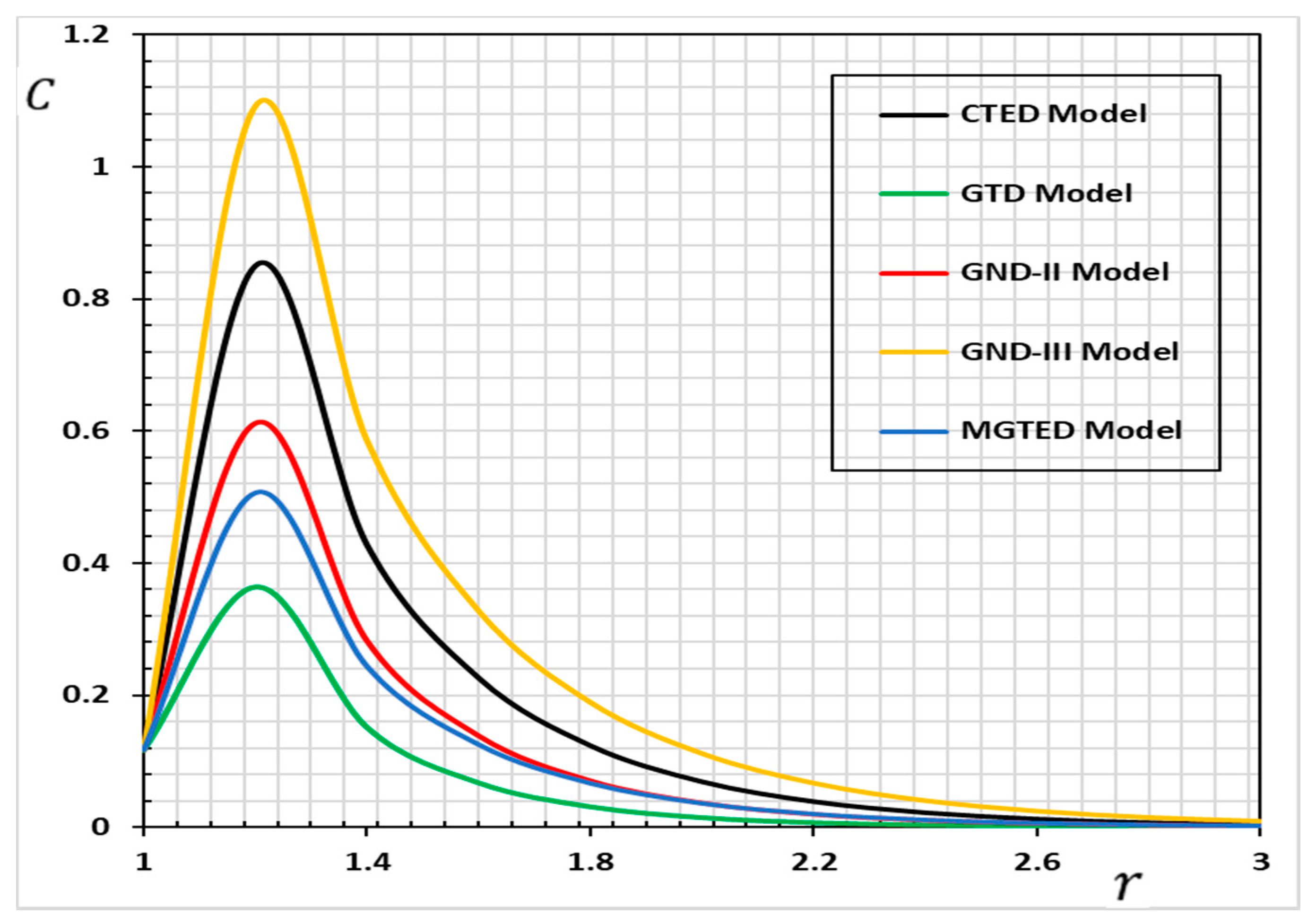
The comparison with space for the distribution of concentration
is shown in
Figure 6 and
Table 6 for different thermos-diffusion models. From the numerical values, it was found that there were some variations between the values of concentration
and the variation in the model. The concentration
curves and tables have the same behavior but vary only in quantity.
The concentration begins with a positive value at the cavity of the cylinder and then rises steadily until reaches its highest local maximum value. After that, increasing the distance r within the medium steadily decreases until it dissipates to obtain its null value. In contrast with the CTED and GND-III models, the -field values can be inferred from the numeric values to be smaller in the case of the MGTED model. The GND-III model, however, gives the GND-II model a larger model.
The medium is strained in the vicinity of the cylinder and, with the passing of time, is greater. Cross-effects may result in the presence of tensile stress near the cavity surface due to temperature coupling, mass dissemination, and strain fields. Owing to these cross-effects, an additional accumulation of thermal stress arises from the thermal excitation. The primary difference between the GND-III model of thermoelastic diffusion and the MGTED-based thermal conductivity equations of thermoelastic diffusion is the additional delay times and .
These relaxation times provide an additional diffusion and propagation mechanism in the governing equation for the dissipation effect. The delay time is known to monitor the propagation behavior of the thermal wave, slow down the speed of heat-wave propagation, and show the characteristics of the thermal wave. Thermal energy can be diffused, and diffusion wave decay characters can be produced in the MGTED heat transfer by the effect.
7. Conclusions
A new generalized thermoelastic diffusion model has been derived in the present paper, connecting heat and mass flux in elastic materials. It is understood that, due to the coupling between temperature and mass diffusion as well as stress fields, thermoelastic diffusion takes place in a flexible solid material. Centered on the Moore–Gibson–Thompson equation, the constitutive equations, as well as the heat and mass diffusion equations, have been modified. The goal behind the implementation of this new model was to deal with the evident inconsistency between the infinite thermal and diffusion rates predicted by the classical theories of thermoelastic diffusion [
1,
33,
34,
35] and the energy dissipation model of Green and Naghdi (GN-III) [
5]. In the constructed modified model, the laws of Fourier and Fick have also been improved to incorporate the time needed to speed up the heat wave and the time derivative of the diffusive mass flow.
The primary distinction between the thermoelastic diffusion model GND-III and the thermoelastic diffusion thermal conductivity equations based on MGTED is the additional delay times and . These relaxation times provide an additional diffusion and propagation mechanism in the governing equation for the dissipation effect. The delay time is known to monitor the propagation behavior of the thermal signal, slow down the speed of thermal wave propagation, and show the characteristics of the thermal wave.
Thermal energy can be diffused, and diffusion wave decay characters can be produced in the MGTED heat transfer by the effect.
The problem of an unbounded solid with a cylindrical cavity with a permeable material shaped on the surface in contact with the cylindrical cavity has been studied to explain and examine the proposed model. In the area of Laplace transformation, the solution is achieved by a direct approach. Centered on Fourier expansion techniques, a computational approach is used to invert Laplace transforms to solve the problem in the physical field.
It was found from our observations that thermal and diffusion waves are propagated as a wave with a slight velocity rather than an endless velocity on the conventional thermoelastic diffusion model. The thermoelastic diffusion models can be deduced as special cases: Green–Naghdi Type II and III models, generalized thermo-diffusion with one relaxation. Furthermore, the GND-III and CTED models have a near-conduct but are distinct from MGTED, which shows that the model of thermoelastic diffusion was significant. The results in this article should be useful for science and engineering research as well as for those working on solid mechanics growth. A wide variety of thermodynamic concerns are related to the method used in this article. These theoretical conclusions will provide experimental experts and researchers who work on this subject with interesting knowledge.


