Abstract
This paper deals with a method for the parameter and order identification of a fractional model. In contrast to existing approaches that can either handle noisy observations of the output signal or systems that are not at rest, the proposed method does not have to compromise between these two characteristics. To handle systems that are not at rest, the parameter, as well as the order identification, are based on the modulating function method. The novelty of the proposed method is that an optimization-based approach is used for the order identification. Thus, even if only noisy observations of the output signal are available, an approximate identification can be performed. The proposed identification method is, then, applied to identify the parameters and orders of a lithium-ion battery model. The experimental results illustrate the practical usefulness and verify the validity of our approach.
1. Introduction
In recent years, fractional models have been increasingly used to describe a broad range of real world problems [1]. Fractional analysis provides models that accurately describe the long-term phenomena of systems as the fractional operators take into account the entire system’s past. In contrast to the integer order operators, the information of the system’s past is not concentrated in the initial conditions; however, the system’s past is represented by a non-constant function [2]. In the context of parameter and order identification, this non-constant function has to be considered, otherwise it leads to incorrect parameter and order identification [3].
To overcome this drawback, the majority of approaches for parameter and order identification assume the system to be at rest (see e.g., [4,5,6,7,8]). This means that the input and output signal are assumed to be zero before the start of the identification. However, fractional models are primarily used to describe long-term phenomena, such as the diffusion process in a lithium-ion battery. For a lithium-ion battery to be considered at rest, this diffusion process must have completely decayed, which can take several hours [9]. Therefore, the assumption that the system is at rest is restrictive in terms of applicability.
In [3,10], two approaches were proposed that dropped the assumption of a system at rest. The authors of [3] applied the Caputo definition for the fractional derivatives. Integrating the underlying fractional differential equation with the highest derivative order leads to the initial values in the system description. These initial values are interpreted as additional parameters of the system and collected in an extended parameter vector. Under the assumption that the fractional orders are known, a method for the bias-free identification of the extended parameter vector under noisy observations of the input and output signal is presented.
A shortcoming of the method from [3] is that the initial values of the Caputo derivatives do not initialize the system properly [11]. Instead, as with the Riemann–Liouville definition, the entire past of the input and output signal has to be taken into account to initialize the Caputo derivative properly [12].
This is considered in the approach of [10], which is based on the findings from [5]. In opposite to [3], not only the parameters but also the orders of the fractional system are identified in the method from [10]. The approach is derived from the modulating function method, which allows elimination of the influence of the entire system past. Even though the approach is demonstrated with a noisy observation of the output signal, the orders are determined by solving a root-finding problem. Thus, the noisy observation of the output signal leads to an ill-posed problem.
To determine the orders in the presence of noise, an optimization-based approach is proposed in this paper. The approach is also based on the modulating function method to keep the possibility of eliminating the influence of the entire system’s past. For the sake of practical implementation, the Grünwald–Letnikov definition is used instead of the Riemann–Liouville definition.
The remainder of this paper is structured as follows: First, Section 2 outlines the preliminaries. In the first part of Section 3, the parameter identification is briefly introduced. The second part of Section 3 presents the order identification under noisy observations of the output signal, which is the first main contribution of the paper. The application to a lithium-ion battery and the identification of the parameters and orders are the second main contribution, which is described in Section 4. In Section 5, we draw the main conclusions from this paper.
2. Preliminaries
In the literature, many definitions for the fractional operator exist. With regard to practical implementation, the presented approach is based on the definition of Grünwald–Letnikov. Further, the fractional model and the identification equation on which the approach is based on are given in this section.
2.1. Fundamentals of Fractional Calculus
Throughout this subsection, and are smooth functions with , for all and , for all . Let , , and with . Furthermore, describes the floor function and denotes the biggest integer smaller or equal to the argument.
All so far mentioned definitions of Caputo, Riemann–Liouville, and Grünwald–Letnikov can be found in, e.g., [13,14,15,16], whose notation is also used in this paper.
Definition 1.
Left-Sided Grünwald–Letnikov Derivative.
The definition of the left-sided Grünwald–Letnikov derivative is
where T is the sampling time.
Definition 2.
Right-Sided Grünwald–Letnikov Derivative.
The right-sided Grünwald–Letnikov derivative is defined as:
where T is the sampling time.
Following the notation of [16], the fractional derivative operators are given by . The derivative order is given as the right upper index . The lower left index for the left-sided case or the lower right index for the right-sided case marks the time before or after the function is zero. The third parameter is the actual time t and is given as lower right respectively left index.
The derivative of the right-sided Grünwald–Letnikov definition with respect to the order is given in the following lemma, which was originally stated in [10].
Lemma 1.
Derivative of the Right-Sided Grünwald–Letnikov Definition.
The derivative of the right-sided Grünwald–Letnikov definition is
The proof can be found in [10].
Remark 1.
Assuming a continuous and bounded function h and a finite sampling time T, then the derivative of the right-sided Grünwald–Letnikov definition (3) does not have singularities and is bounded.
2.2. Fractional Model
Consider the general non-commensurable fractional model
where is the time-continuous input signal and is a noisy observation
of the noise-free output signal y, which is superimposed by a white noise with a zero mean. The derivative operator indicates that the system is not at rest. marks that the system is interpreted in terms of Riemann–Liouville [13,14,15]. The unknown parameters are collected in the vector
where , and the fractional orders in the vector
where , and . Without loss of generality, the fractional orders are assumed to be ordered , with . The number of unknown parameters are assumed to be known.
Regarding the noise , the input signal u, the output signal , and the parameters , the following assumptions are made.
Assumption 1.
Noise Properties.
We assume white noise ϵ with zero mean
where E denotes the expectation, σ denotes a constant, and δ denotes the Dirac delta function (see ([17], p. 56)).
Assumption 2.
Bounded Signals.
The input u and output signal are assumed to be bounded.
Assumption 3.
Parameter Normalization.
Without loss of generality, the normalization holds in (4).
2.3. Simulation of a Fractional Model
In the parameter identification method, a simulation of the system output signal y is needed. To simulate a fractional model (4), a closed-form solution with zero initial conditions is given in [18] (p. 113). In general, if the system is not at rest and, hence, no zero initial conditions are present, an error between the simulated output signal with and without zero initial conditions occurs [19]. To reduce this error, an extension based on a closed form solution that considers the latest past of the system in sense of the short-memory principle [20] is proposed in [19].
Definition 3.
Closed-Form Solution Considering the Short-Memory Principle.
A closed-form solution that considers the short-memory principle is defined as:
where T is the sampling time, is the time where the measurement starts, is the time where the simulation starts, and L is the memory length.
Remark 2.
For the definition 3, it is assumed that the system is at rest before .
The input signal u and the output signal of the system y in are used to initialize the closed-form solution (10). From onward, the simulation of the system output signal is calculated recursively.
2.4. Modulating Function Method and Identification Equation
The modulating function method was first proposed in [21]. The basic idea is to transfer the derivatives of the initial signals to an arbitrary and continuously differentiable function by means of integration by parts. Therefore, the fractional model (4) is multiplied with a function that is continuously differentiable. The resulting products of the function and the input as well as output signal are integrated over . Applying integration by parts leads to the result that the derivatives are swapped but at the expense of arising boundary terms.
Definition 4.
Modulating Function [21].
With regard to a fractional model (4), a modulating function is a function satisfying
The property ensures that all necessary derivatives of the modulating function exist. The property eliminates the boundary terms which arise due to the integration by parts. Considering a third property, viz.
which is stated in [22]. The identification of the modulating function method for a fractional model with initialized derivative operators results in
The derivatives of the model (4) are considered to be described by the fractional operator of Riemann–Liouville. Applying the modulating function method, the derivative type changes to the Caputo definition for the modulating function [22]. Therefore, the approach can be formulated using the Grünwald–Letnikov derivative, and the Caputo definition has to be replaced by the Grünwald–Letnikov definition. If the modulating function is -times continuously differentiable, the derivative operator of Riemann–Liouville and Grünwald–Letnikov are interchangeable [23]. The Riemann–Liouville derivative is linked with the Caputo derivative through ([24], p. 91)
3. Combined Iterative Parameter and Order Identification
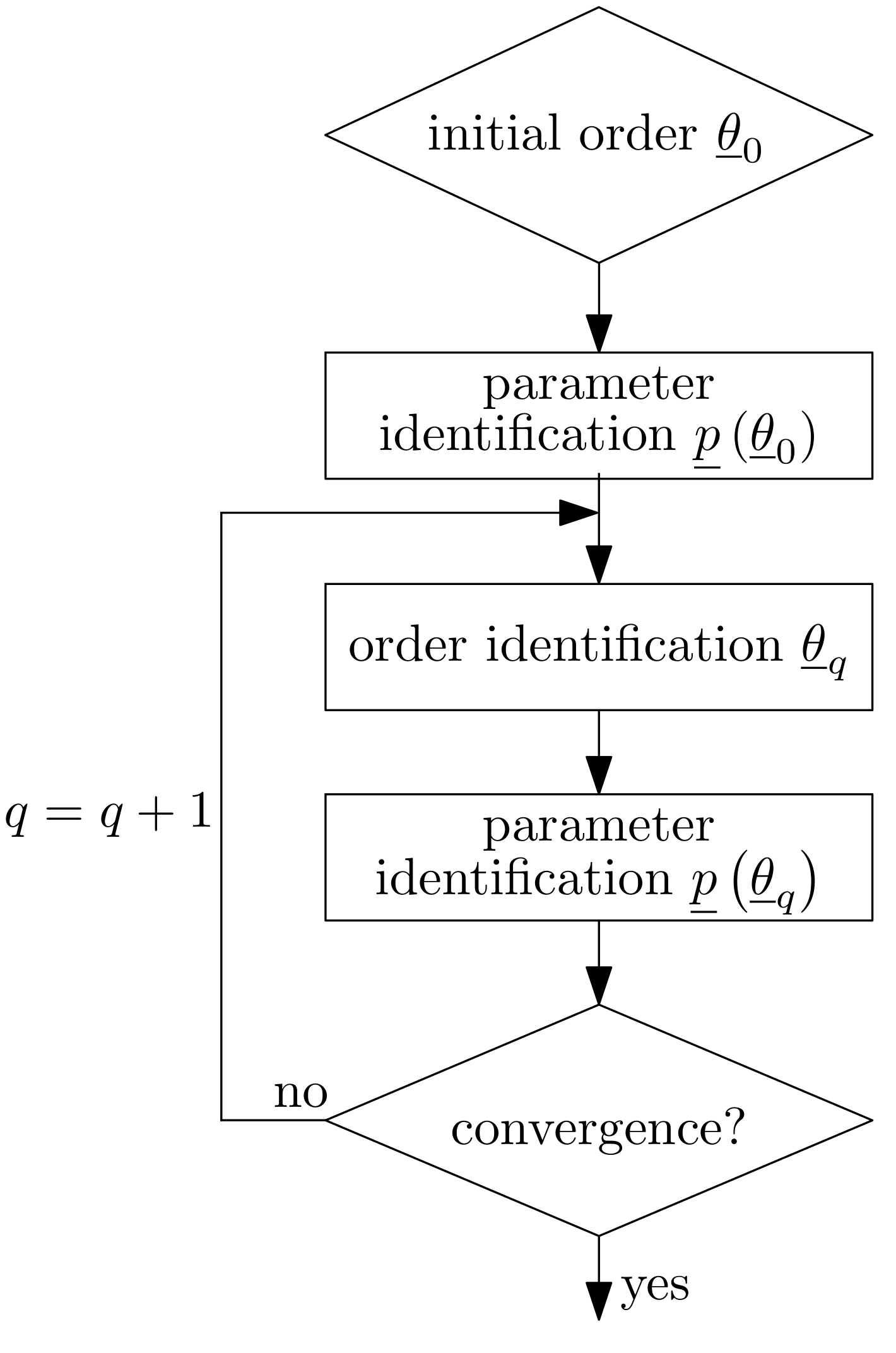
In this section, a method for parameter and order identification is introduced. The novelty is that the method can handle noisy observations of the output signal. The identification is performed iteratively whereby the orders are updated in a first step, and afterwards the parameters are identified for the orders of the actual iteration. This procedure is shown in Figure 1. For a consistent parameter estimation under noisy measurements, we apply the approach from [19]. This approach is outlined in Section 3.1. The focus of the paper is on the order identification under noisy observations of the output signal. Instead of solving a root-finding problem, as in [10], an optimization-based approach is used to identify the derivative orders of a fractional model (4). This main contribution of the paper is given in Section 3.2.

Figure 1.
Iterative method for simultaneous parameter and order identification of a fractional model.
3.1. Parameter Identification
The method introduced in [19] is an extension of the instrumental variable method for integer order models to fractional order models. To apply the instrumental variable method, we require identification equations, where is the number of model parameters. The identification equations are generated by evaluating the integrals in (13) for different time intervals. In general, the lower bound of the integral can be expressed by and the upper bound by where . These time points can be derived, e.g., by shifting the integrals by a fixed time . Assuming that the identification process is started at and the fixed integral width is , the lower and the upper bound are given by and , respectively.
Let Assumption 3 hold. If the derived identification equations are independent, the linear system
is set up for the parameter identification. The parameters depend on the latest estimates of . The vector describes the -th fractional derivative of the modulated output signal
The measurement matrix consists of the vectors , which are the remaining modulated derivatives of the output and input signal:
where . Due to the noisy observations of the output signal, the least-squares method leads to biased estimates of the parameters [25]. Therefore, a matrix of instrumental variables where
is used to solve the linear system (14):
Instead of the noisy observations of the system output signal , the simulation of the output signal is used to set up (17). Thus, the instrumental variables fulfill the requirements of the instrumental variable method in that they are uncorrelated to the noise but strongly correlated to the undisturbed input signal and output signal of the system.
The approach can be summarized as follows:
- The parameters are estimated using the least-squares method after N iterations where N is the number of parameters for the first time.
- These parameters are used to simulate the output signal with the current fractional orders . In general, the entire past of the system is not available. Thus, the closed-form solution based on the short-memory principle (10) is used to calculate .
- The calculated output signal is used to set up the instrumental variable matrix and to refine the parameter estimates iteratively via (18) until a maximum number of iterations is reached or the difference between the two estimates is almost zero.
3.2. Order Identification
For the parameter identification, we assumed that the derivative orders are available in each iteration. In this subsection, an order identification method is proposed. Therefore, the identification equation of the modulating function (13) is interpreted as a nonlinear function that depends on the orders of the system
For a noisy output signal, the nonlinear equation for the order identification results in
In the sequel, we first investigate the influence of the noise on the order identification. Afterwards, an optimization-based method for the order identification is proposed, and the combination with the parameter identification is outlined.
3.2.1. Ill-Posed Root-Finding Problem
For the original parameters and and the orders and of the model, is zero. In [10], this fact is used to transfer the order determination into a root-finding problem. In contrast to , in general, f is not zero for the original parameters and orders but takes the value
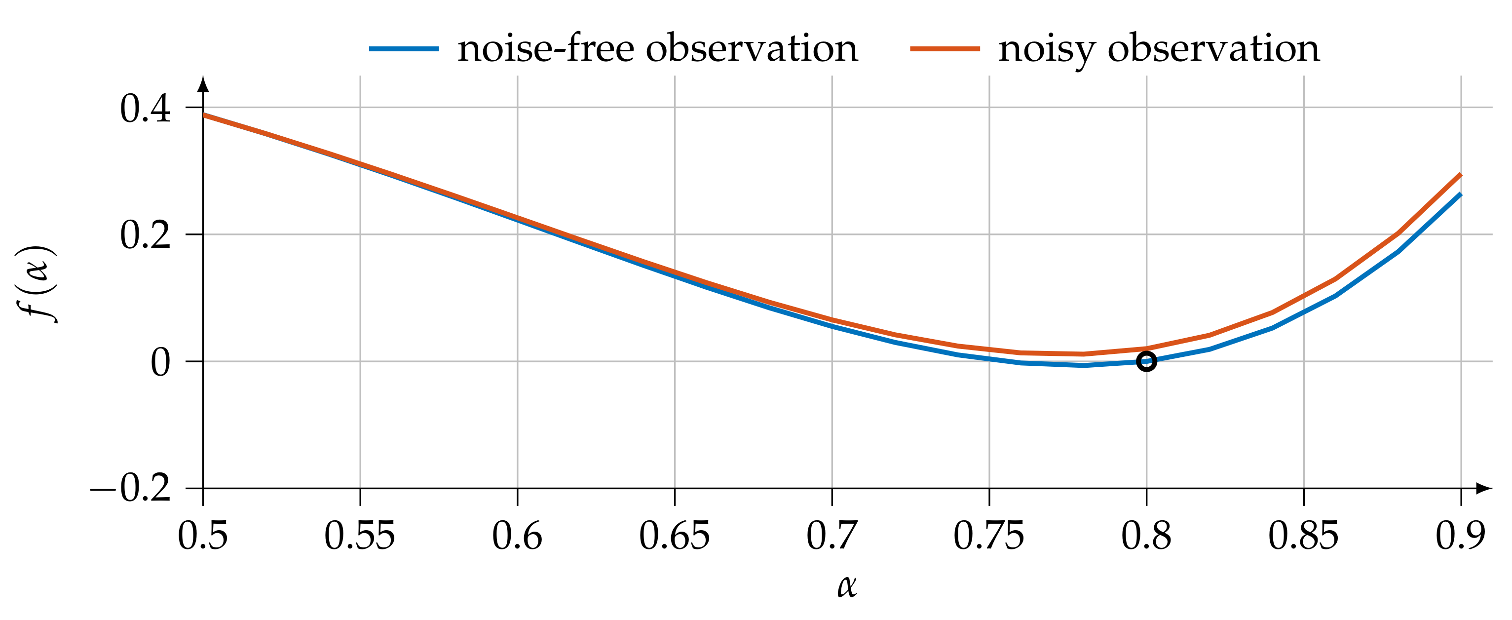
It is possible that, for small deviations of the original parameters and orders, f is zero. However, the possibility also exists that f is always different from zero. In this case, an identification of the orders using root-finding algorithms is not possible. This is exemplified in Figure 2. A system described by
where , and is excited with a pseudo random binary signal. The identification Equation (20) is evaluated in a brute-force manner for , while the parameters are kept at and . The first evaluation is performed with the noise-free output signal, which is represented by the blue line in Figure 2. The red line, on the other hand, is obtained from an output signal, which is superposed by a time-variant noise . The root disappears in this case, and thus the order can not be derived by the approach proposed in [10].
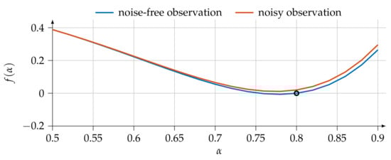
Figure 2.
Visualizing the influence of the noise on the identification equation.
3.2.2. Optimization-Based Approach
In order to identify at least the derivative orders in the presence of noisy observations of the output signal approximately, an objective function
where is defined. As can be seen, the objective function is formulated in the sense of best fitting. In (24), the function
includes independent equations derived from (20). Equation (25) can be obtained from shifting the integral as described in Section 3.1.
To identify the orders, the objective function has to be minimized with respect to the orders:
The optimization problem (26) is solved using the Gauß–Newton method ([26], S. 214 ff.).
where is the gradient:
and is the approximated Hessian of the Gauß–Newton method:
3.2.3. Convergence Analysis
In this subsection, the derivative of the order identification Equation (20) is calculated first. This derivative is needed for gradient (28) as well as Hessian (29). Secondly, the convergence of the Gauß–Newton method for the stated problem (26) with (24) is analyzed.
Lemma 2.
Partial Derivative of Order Identification Equation (25).
Suppose , , and an independent equation (25) of f in (20). Further, let describe the j-th element of the order vector in (7).
The partial derivative of with respect to is
where
In (31), the partial derivative of the Grünwald–Letnikov derivative is given in Lemma 1.
Proof.
If (25) is derived with respect to , it must be considered that the parameters as well as the derivative of Grünwald–Letnikov depend on the orders. To calculate the derivative, the product rule is used. While the parameters depend on all orders and are stated in (30), the Grünwald–Letnikov derivatives only depend on one specific order. Therefore, a case distinction depending on the derivative order has to be performed, which is given in (31). The needed derivative of the Grünwald–Letnikov derivative with respect to the order is given in Lemma 1. □
The derivatives of the parameter and in (30) depend on the specific method for the parameter identification. In this paper, the instrumental variable method from [10] is used to achieve a consistent parameter estimation. Based on the parameter identification Equation (18), the corresponding partial derivative of the parameters is calculated.
Lemma 3.
Partial Derivative of the Parameter.
is the instrumental variable matrix with
and is the measurement vector with
Further, let describe the j-th element of the order vector (7).
The partial derivative of with respect to can be calculated as
Proof.
Starting from the linear system (14), the first step is the multiplication of the linear system (14) with the transposition of the instrumental variable matrix
Deriving (37) with respect to yields
To obtain this equation, the product rule is used. Equation (38) is rearranged such that all expressions except for the expression depending on the partial derivative of the parameter are on one side
Under the assumption of independent equations for the parameter identification problem, the inverse of must exist. Otherwise, the requirements for the parameter identification are not met. The inversion of is the last step to calculate the derivative of the parameters. □
Due to the computational effort of the non-recursive instrumental variable method, often the recursive realization is used in practical applications ([17], p. 269). In this case, (36) cannot be calculated, and the difference quotient is used to approximate the derivative of the parameters. As an example, the difference quotient for the -th element of the parameter vector and the j-th element of the order vector result in
where , . In (40), is a sufficiently small constant that represents the difference interval. The vector is the j-th unit vector of and is used to select the element of the vector .
Under the assumption that the Hessian is non-singular, the Hessian of the Gauß–Newton method is a positive definite matrix ([26], S. 215). Hence, if the derivatives exist and has no singularity, the Gauß–Newton method converges.
Lemma 4.Convergence Analysis.
- (a)
- the sampling time T is finite, and
- (b)
- the modulating function γ,
- (c)
- the input signal u, the output signal , the parameters and , and the derivatives of the parameters and are bounded.
Proof.
If the sampling time is equal to zero, the partial derivative of the Grünwald–Letnikov definition (3) has a singularity. Due to this, the sampling time must be restricted to finite values, which is ensured by requirement (a).
With regard to practical applications, the requirements (a)–(c) are not restrictive. The requirement (a) is always fulfilled for implementation on processing units. The fulfillment of requirement (b) can be ensured by the choice of the modulating function without any restriction by the properties and . The boundedness of the input signal, output signal, parameters, and the derivatives of the parameters regardless of the chosen method is guaranteed by the practical Assumption 2, which fulfills requirement (c) [19]. However, the Gauß–Newton method generally does not ensure that the global minimum is reached. This results from the fact that the Gauß–Newton method is based on a linear approximation of the original problem. The minimum the Gauß–Newton method converges against depends on the chosen initial solution and on the specific nonlinearity ([26], S. 214 ff.).
4. Parameter and Order Identification for a Model of a Lithium-Ion Battery
In this section, the proposed parameter and order identification approach is applied to a lithium-ion battery model. To this end, it is crucial that the modulating function satisfies property as, otherwise, the system is required to be at rest. Considering the lithium-ion battery, the diffusion process has to decay, which can take several hours. The choice of such a modulating function is stated in Section 4.1. In Section 4.2, the fractional model of a lithium-ion battery is given, and the experimental setup is explained in Section 4.3. The ground truth for the identification is determined in Section 4.4. The identification is carried out in Section 4.5.
4.1. Choice of Modulating Function
One advantage of the approach from Section 3 is that the system need not to be at rest at the beginning of the identification process. This advantage is at the cost of the modulating function fulfilling property in addition to and . In [22], they proved that the spline-type modulating function also fulfilled property .
Definition 5.
Spline-Type Modulating Function [27].
The spline-type modulating function is the integration over a weighted sequence of impulses
where is the number of splines, and represents the order of the modulating function.
4.2. Model of a Lithium-Ion Battery
Several models to describe a lithium-ion battery exist in the literature. Depending on the modeling goal, the range is from detailed electrochemical models to behavior models, see [28,29]. The electrochemical models are based on particle models, and partial differential equations are used, whereas the behavior models are described by circuits. Fractional models are a compromise between the electrochemical models and behavior models, see [30] (p. 141 ff.) and [16,29,31,32]. In general, the fractional impedance model of a lithium-ion battery is used to describe the overvoltages of the different loss processes and the overvoltage of the diffusion process in a lithium-ion battery [31].
The model
where s depicts the complex number frequency parameter and is the fractional order used in this paper is based on [29]. Due to the minimal sampling time is realizable with the experimental setup, which is explained in the next subsection, and only the low frequency range of the model proposed in [29] can be correctly reconstructed. The loss processes of the high and mid frequency range are collected in . The differential capacity describes the amount of charge that has to be removed or inserted to change the open circuit voltage (OCV) by a specified quantity [33]:
For the parameter and order identification, the model (42) has to be rearranged so that it appears in the form of (4). First, the fractions are extended
Second, using the Laplace transform ([13], p. 79) yields
Due to Assumption 3, (45) is divided by
4.3. Experimental Setup
Due to safety reasons, the lithium-ion battery was operated in a climate chamber VC3 4018 from Vötsch. The lithium-ion battery was excited with a BOP 20-20M from Kepco, and the excitation was realized as a current excitation. The current was measured with a digital multimeter 34410A from Agilent, which had a standard deviation of . The voltage was measured with a DS2004 High-Speed A/D Board from dSpace. The DS2004 High-Speed A/D Board was integrated in a real-time system and had a standard deviation of .
The data transfer of the multimeter to the host computer took . While the data were transferred, no new data could be recorded from the multimeter. To avoid an incorrect parameter and order identification due to measurement losses, the sampling time was chosen to be .
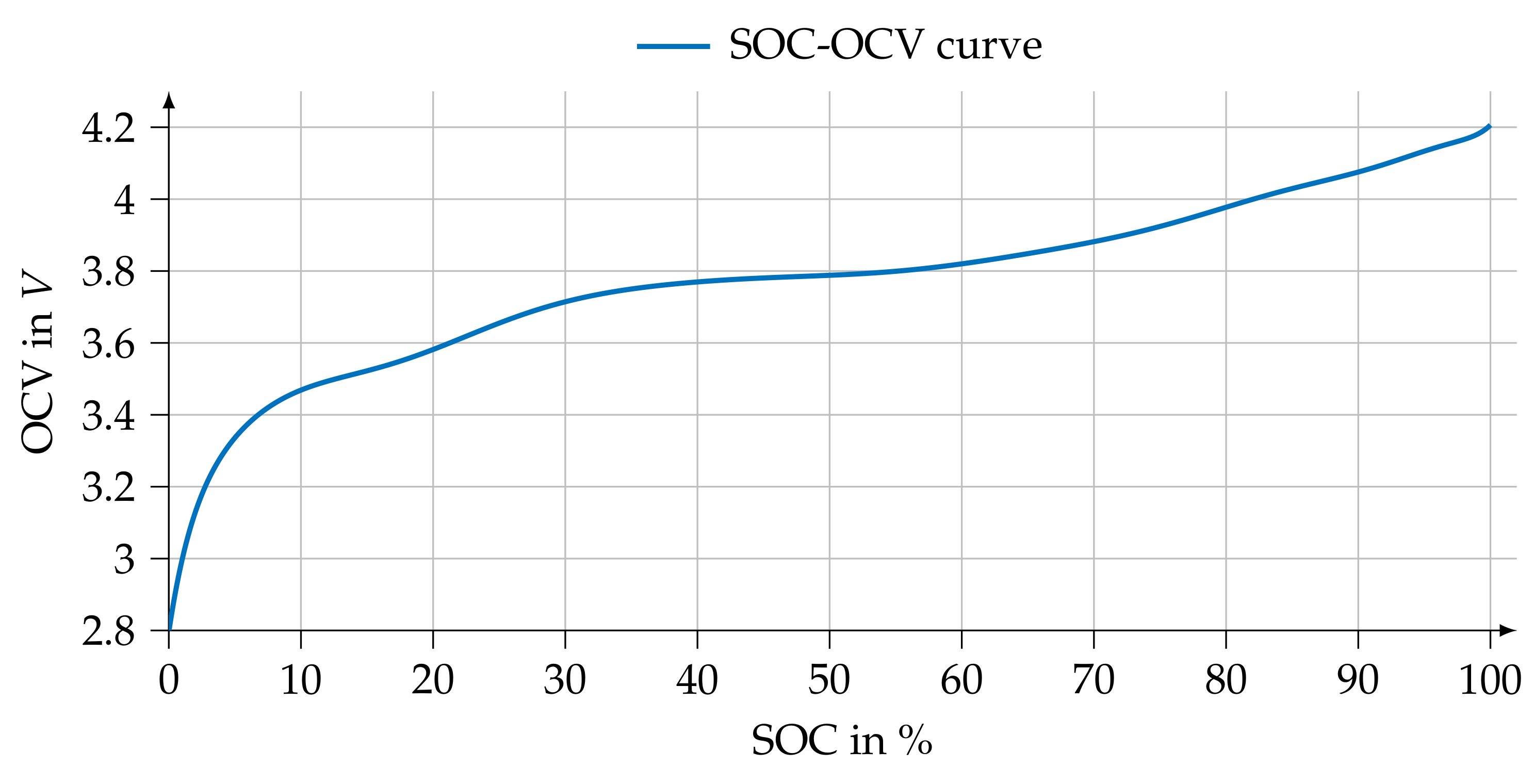
The measurement was recorded in a voltage-correct circuit, which is shown in Figure 3. With this, it is taken into account that the parameters and orders of the fractional model of the lithium-ion battery (44) depended on the OCV and were only valid for small-signal excitation ([9], p. 63 f.). To achieve a consistent parameter identification, the measured voltage had to be corrected by the instantaneous OCV ([17], p. 255). A current-correct circuit leads to systematic errors in voltage measurements, such that the correction of the measured voltage is also incorrect. Even if the voltage across the ammeter is very low, the voltage drop suggests a great change in the state of charge (SOC), especially in the range of [40%, 60%]. This is due to the flat course of the SOC-OCV curve, see Figure 4.
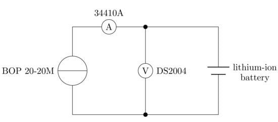
Figure 3.
Schematic illustration of the measurement setup for the parameter and order identification of a lithium-ion battery model.
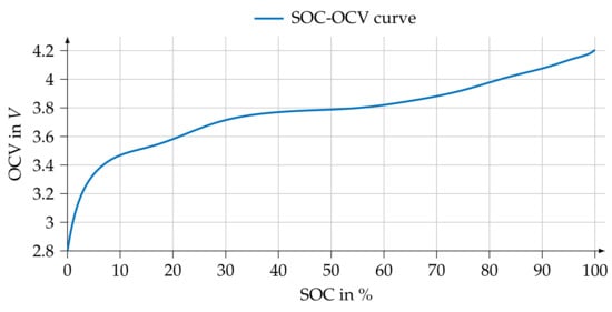
Figure 4.
Relation between the state of charge (SOC) and open circuit voltage (OCV) for the used lithium-ion battery of type SLPB 834374H.
4.4. Experiment and Ground Truth
The fractional battery model (44) is only valid in a single operating point, which depends on the temperature and state of charge. To prevent any changes from the operating point due to temperature changes, the temperature was kept constant at inside the climate chamber. Thus, the state of charge was not varied during the measurement. A pseudo random binary signal with a pulse duration of with the following two properties was used. The first property concerns the peak-to-peak amplitude, which was chosen as . Next to this, the pseudo random binary signal was designed such that it was zero mean over the entire measuring range.
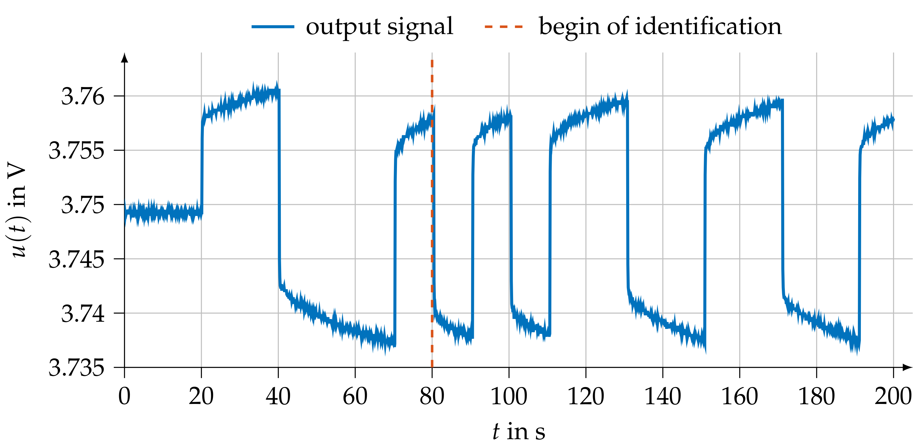
The measured input signal is shown in Figure 5, and the measured output signal of the lithium-ion battery is shown in Figure 6. In both figures, a dashed red line indicates the point in time from which the data were used for the combined parameter and order identification. The data before were only available for the determination of the reference parameters.
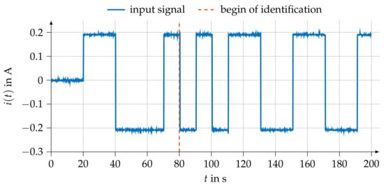
Figure 5.
Input current measured with the digital multimeter 34410A and used as the input signal for the parameter and order identification of the fractional battery model (44).
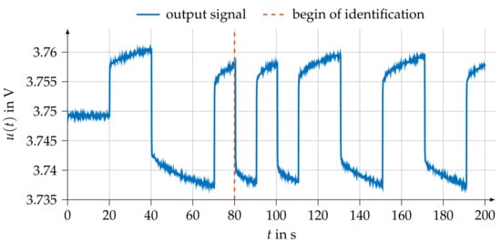
Figure 6.
Output voltage measured with the DS2004 High-Speed A/D Board and used as the output signal for the parameter and order identification of the fractional battery model (44).
The lithium-ion battery was not excited for the first to check if the lithium-ion battery was at rest and to determine the instantaneous OCV. As the standard deviation of the measurement is comparable to the standard deviation of the manual , we assumed that the lithium-ion battery was at rest. The OCV was calculated as mean value of the first and was
In combination with Figure 4, the SOC was determined to be 34.9%. Considering (43), the corresponding differential capacity can be derived from the SOC-OCV curve. The differential capacity is equivalent to the reciprocal of the derivative of the SOC-OCV curve. With the given SOC-OCV curve (cf. Figure 4) and SOC value, the differential capacity was determined as
The parameter to be identified is
The parameter and the order are estimated by a complex nonlinear least squares regression. As an objective function, the quadratic error between a simulated output signal and the measured output signal is used. For the simulation, the complete input signal is used. Thus, we ensured that the system was at rest and no error occurred in the parameter and order due to neglecting a part of the system’s history.
4.5. Results of the Combined Parameter and Order Identification
The instrumental variable method as described in Section 3.1 was applied for the parameter identification. To set up the instrumental variables, a simulated output signal is needed. The closed-form solution (10) considering the short-memory principle was used so that a strong correlation was achieved with the undisturbed output signal, but the whole past of the system did not have to be taken into account. The memory length was chosen to be . The less computationally expensive recursive instrumental variable method instead of the non-recursive method was applied. Hence, an initial covariance matrix must be provided. As two parameters have to be identified, the covariance matrix is a matrix and is chosen to be
The values in (50) are motivated by the very small reference parameters. Before the identification can be performed, the spline-type modulating function (41) has to be parameterized. The number of splines was chosen to be , and the order was . The identification horizon was . Further, to generate independent Equation (25), the start of the integral is shifted by for each equation.
For the first parameter identification and, hence, before the iterative parameter and order identification is started (see Figure 1), the first two iterations within the parameter identification are performed in sense of the least-squares method as described at the end of Section 3.1. After the first two iterations, the output signal is simulated using the actual estimates of the parameters and the instrumental variables are calculated for the parameter identification. Within the iterative parameter and order identification (), the parameters of the iteration before () are used to set up the instrumental variables for the first iteration of the parameter identification. Afterwards, the updated estimates are always used.
As in the case of parameter identification, the identification Equation (25) of the order identification is also based on the modulating function method. The spline-type modulating function with the same parameterization as for the parameter identification is used. The initial value of the order is specified to be . Since the identification is performed in the non-recursive form, the derivative of the parameters can not be calculated analytically. Instead, the numerical approximation (40) is used. The deviation from the derivation order of the actual iteration, which is required to evaluate the difference quotient, is set to (see (40)).
The iterative character of the parameter identification and of the combined parameter and order identification approach makes stopping criteria necessary. In this paper, two stopping criteria were formulated for each iteration. One stopping criterion is the maximum number of iterations . The maximum number of iterations is limited by the measurement duration (cf. Figure 5 and Figure 6), the memory length L in combination with the sampling time T, and the chosen identification horizon and shifting time of the modulating function method. Using the chosen data, the maximum number of iterations is
A second stopping criterion considers the change of the estimated parameter and orders between two consecutive iterations. If the change of the parameters is smaller than , the instrumental variable method terminates, and the next step of the order identification is performed. If the change of the order is smaller than , the combined parameter and order identification process terminates.
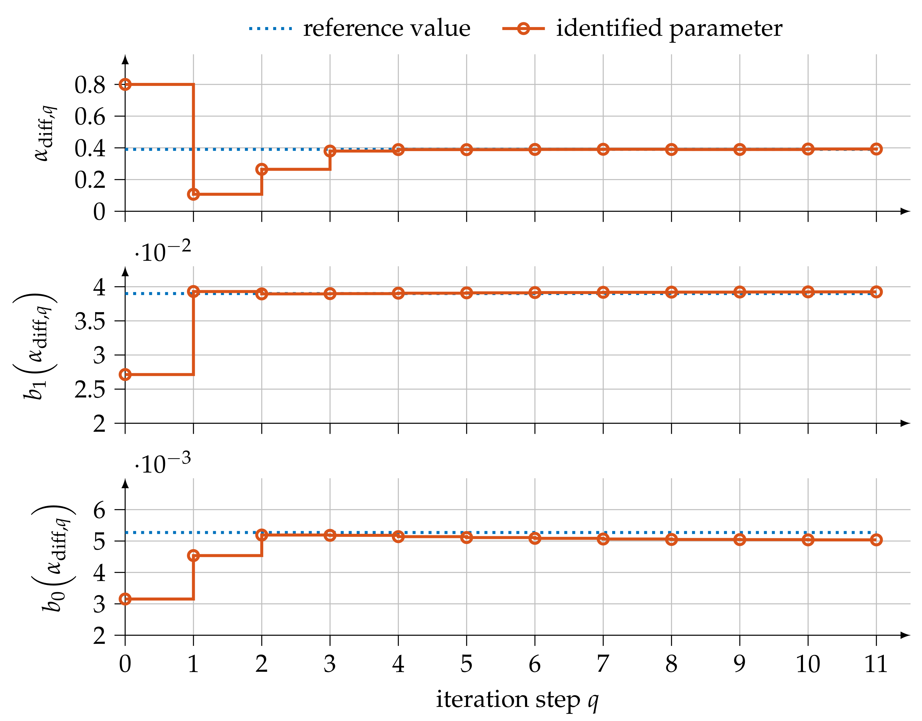
To distinguish the identified parameters from the reference parameters, these are denoted as . The notation is used to mark the identified order. The identification results are presented in Figure 7. The reference parameters, which were determined in the section before, are illustrated as dotted blue lines, while the identified parameters and orders are given as a solid red line. Even though only noisy observations of the input and output signal are available, all parameters and the order converge against the reference values. Nonetheless, the exact values are not reached within the considered time. This is in line with the discussion about the influence of the noise on the nonlinear equation for the order identification in Section 3.2. The relative error after termination, i.e., the relative error between the data of the eleventh iteration and reference values, for the parameters are

Figure 7.
The identification results of the proposed method for a lithium-ion battery using real measurements.
5. Conclusions
In this paper, a combined parameter and order identification method for fractional systems under noisy observations of the output signal was proposed.
The order identification was performed by an optimization-based approach that relied on the modulating function method. The optimization-based approach ensured the order identification to be robust against measurement noise. The parameter identification was based on the instrumental variable approach from [19]. In contrast to the methods from the literature, our method did not require the system to be at rest at the beginning of the identification process. Furthermore, we provided practical implementable expressions of the necessary equations and derivatives, which were derived in analytical form.
We applied the combined identification method to a fractional model of a lithium-ion battery. The experimental results revealed that the proposed method yielded the correct parameters in the presence of noisy observations of the output and input signal. These identification results demonstrated that the method was practically applicable.
Author Contributions
Conceptualization, O.S.; methodology, O.S.; software, O.S.; validation, O.S. and M.P.; investigation, O.S. and M.P.; resources, S.H.; writing—original draft preparation, O.S.; writing—review and editing, M.P. and S.H.; visualization, O.S.; supervision, S.H. All authors have read and agreed to the published version of the manuscript.
Funding
We acknowledge the support of the KIT-Publication Fund of the Karlsruhe Institute of Technology.
Institutional Review Board Statement
Not applicable.
Informed Consent Statement
Not applicable.
Data Availability Statement
Not applicable.
Conflicts of Interest
The authors declare no conflict of interest.
Abbreviations
The following abbreviations are used in this manuscript:
| C | Caputo |
| GL | Grünwald–Letnikov |
| OCV | open circuit voltage |
| RL | Riemann–Liouville |
| SOC | state of charge |
References
- Kanth, A.S.V.R.; Garg, N. Computational simulations for solving a class of fractional models via Caputo-Fabrizio fractional derivative. Procedia Comput. Sci. 2018, 125, 476–482. [Google Scholar] [CrossRef]
- Sabatier, J.; Merveillaut, M.; Malti, R.; Oustaloup, A. How to impose physically coherent initial conditions to a fractional system? Commun. Nonlinear Sci. Numer. Simul. 2010, 15, 1318–1326. [Google Scholar] [CrossRef]
- Lu, Y.; Tang, Y.; Zhang, X.; Wang, S. Parameter identification of fractional order systems with nonzero initial conditions based on block pulse functions. Measurement 2020, 158, 107684. [Google Scholar] [CrossRef]
- Aldoghaither, A.; Liu, D.Y.; Laleg-Kirati, T.M. Modulating functions based algorithm for the estimation of the coefficients and differentiation order for a space-fractional advection-dispersion equation. SIAM J. Sci. Comput. 2015, 37, 2813–2839. [Google Scholar] [CrossRef] [Green Version]
- Belkhatir, Z.; Laleg-Kirati, T.M. Parameters and fractional differentiation orders estimation for linear continuous-time non-commensurate fractional order systems. Syst. Control Lett. 2018, 115, 26–33. [Google Scholar] [CrossRef] [Green Version]
- Rapaić, M.R.; Pisano, A.; Jeličić, Z.D. Adaptive order and parameter estimation in fractional linear systems by approximate gradient and least squares methods. IFAC Proc. Vol. 2013, 46, 881–886. [Google Scholar] [CrossRef]
- Tang, Y.; Liu, H.; Wang, W.; Lian, Q.; Guan, X. Parameter identification of fractional order systems using block pulse functions. Signal Process. 2015, 107, 272–281. [Google Scholar] [CrossRef]
- Victor, S.; Malti, R.; Garnier, H.; Oustaloup, A. Parameter and differentiation order estimation in fractional models. Automatica 2013, 49, 926–935. [Google Scholar] [CrossRef]
- Illig, J. Physically Based Impedance Modelling of Lithium-Ion Cells. Ph.D. Thesis, Karlsruher Institut für Technologie (KIT), Karlsruhe, Germany, 2014. [Google Scholar]
- Stark, O.; Karg, P.; Hohmann, S. Iterative method for online fractional order and parameter identification. In Proceedings of the 2020 59th IEEE Conference on Decision and Control (CDC), Jeju, Korea, 14–18 December 2020; pp. 5159–5166. [Google Scholar]
- Sabatier, J.; Farges, C. Comments on the description and initialization of fractional partial differential equations using Riemann–Liouville’s and Caputo’s definitions. J. Comput. Appl. Math. 2018, 339, 30–39. [Google Scholar] [CrossRef]
- Podlubny, I.; Skovranek, T.; Vinagre Jara, B.M.; Petras, I.; Verbitsky, V.; Chen, Y. Matrix approach to discrete fractional calculus III: Non-equidistant grids, variable step length and distributed orders. Philos. Trans. R. Soc. A Math. Phys. Eng. Sci. 2013, 371, 20120153. [Google Scholar] [CrossRef] [PubMed]
- Podlubny, I. Fractional Differential Equations; Academic Press: Cambridge, MA, USA, 1998. [Google Scholar]
- Pooseh, S.; Almeida, R.; Torres, D.F.M. Discrete direct methods in the fractional calculus of variations. Comput. Math. Appl. 2013, 66, 668–676. [Google Scholar] [CrossRef] [Green Version]
- Samko, S.G.; Kilbas, A.A.; Marichev, O.I. Fractional Integrals and Derivatives: Theory and Applications, 1st ed.; CRC Press: Philadelphia, PA, USA, 1993. [Google Scholar]
- Eckert, M.; Kölsch, L.; Hohmann, S. Fractional algebraic identification of the distribution of relaxation times of battery cells. In Proceedings of the 54th IEEE Conference on Decision and Control (CDC), Osaka, Japan, 15–18 December 2015; pp. 2101–2108. [Google Scholar]
- Isermann, R.; Münchhof, M. Identification of Dynamic Systems: An Introduction with Applications; Springer: Berlin/Heidelberg, Germany, 2011. [Google Scholar]
- Xue, D. Fractional-Order Control Systems, Fundamentals and Numerical Implementations; De Gruyter: Berlin, Germany; Boston, MA, USA, 2017. [Google Scholar]
- Stark, O.; Pfeifer, M.; Krebs, S.; Hohmann, S. Bias-free parameter identification for non-commensurable fractional systems. In Proceedings of the 2020 European Control Conference (ECC), St. Petersburg, Russia, 12–15 May 2020; pp. 1422–1429. [Google Scholar]
- Wei, Y.; Chen, Y.; Cheng, S.; Wang, Y. A note on short memory principle of fractional calculus. Fract. Calc. Appl. Anal. 2017, 20, 1382–1404. [Google Scholar] [CrossRef]
- Shinbrot, M. On the Analysis of Linear and Nonlinear Dynamical Systems from Transient-Response Data; Technical Report; National Advisory Committee for Aeronautics: Moffett Field, CA, USA, 1954; Available online: https://digital.library.unt.edu/ark:/67531/metadc57235/ (accessed on 6 July 2021).
- Stark, O.; Kupper, M.; Krebs, S.; Hohmann, S. Online parameter identification of a fractional order model. In Proceedings of the 57th IEEE Conference on Decision and Control (CDC), Miami, FL, USA, 17–19 December 2018; pp. 2303–2309. [Google Scholar]
- Diethelm, K. The Analysis of Fractional Differential Equations: An Application-Oriented Exposition Using Differential Pperators of Caputo Type; Springer: Berlin/Heidelberg, Germany, 2010. [Google Scholar]
- Kilbas, A.A.; Srivastava, H.M.; Trujillo, J.J. Theory and Applications of Fractional Differential Equations, 1st ed.; North-Holland Mathematics Studies: Amsterdam, The Netherlands, 2006. [Google Scholar]
- Dai, Y.; Wei, Y.; Hu, Y.; Wang, Y. Modulating function-based identification for fractional order systems. Neurocomputing 2016, 173, 1959–1966. [Google Scholar] [CrossRef]
- Aragón, F.J.; Goberna, M.A.; López, M.A.; Rodríguez, M.M. Nonlinear Optimization; Springer International Publishing: Cham, Switzerland, 2019. [Google Scholar]
- Maletinsky, V. “l-i-P” Identifikation Kontinuierlicher Dynamischer Prozesse. Ph.D. Thesis, ETH Zurich, Zürich, Switzerland, 1978. [Google Scholar]
- Sabatier, J.; Francisco, J.M.; Guillemard, F.; Lavigne, L.; Moze, M.; Merveillaut, M. Lithium-ion batteries modeling: A simple fractional differentiation based model and its associated parameters estimation method. Signal Process. 2015, 107, 290–301. [Google Scholar] [CrossRef]
- Hu, M.; Li, Y.; Li, S.; Fu, C.; Qin, D.; Li, Z. Lithium-ion battery modeling and parameter identification based on fractional theory. Energy 2018, 165, 153–163. [Google Scholar] [CrossRef]
- Cattani, C.; Srivastava, H.M.; Yang, X.J. Fractional Dynamics; De Gruyter: Berlin, Germany; Boston, MA, USA,, 2016. [Google Scholar]
- Gantenbein, S.; Weiss, M.; Ivers-Tiffée, E. Impedance based time-domain modeling of lithium-ion batteries: Part I. J. Power Sources 2018, 379, 317–327. [Google Scholar] [CrossRef]
- Zou, C.; Zhang, L.; Hu, X.; Wang, Z.; Wik, T.; Pecht, M. A review of fractional-order techniques applied to lithium-ion batteries, lead-acid batteries, and supercapacitors. J. Power Sources 2018, 390, 286–296. [Google Scholar] [CrossRef] [Green Version]
- Schönleber, M.; Ivers-Tiffée, E. The distribution function of differential capacity as a new tool for analyzing the capacitive properties of lithium-ion batteries. Electrochem. Commun. 2015, 61, 45–48. [Google Scholar] [CrossRef]


Publisher’s Note: MDPI stays neutral with regard to jurisdictional claims in published maps and institutional affiliations. |
© 2021 by the authors. Licensee MDPI, Basel, Switzerland. This article is an open access article distributed under the terms and conditions of the Creative Commons Attribution (CC BY) license (https://creativecommons.org/licenses/by/4.0/).