Article

Multi-Objective Optimum Design and Maintenance of Safety Systems: An In-Depth Comparison Study Including Encoding and Scheduling Aspects with NSGA-II

Instituto Universitario de Sistemas Inteligentes y Aplicaciones Numéricas en Ingeniería (SIANI), Universidad de Las Palmas de Gran Canaria (ULPGC), Campus Universitario de Tafira Baja, 35017 Las Palmas de Gran Canaria, Spain
*
Author to whom correspondence should be addressed.
Mathematics 2021, 9(15), 1751; https://doi.org/10.3390/math9151751
Submission received: 30 June 2021 / Revised: 21 July 2021 / Accepted: 22 July 2021 / Published: 25 July 2021
(This article belongs to the Special Issue Evolutionary Algorithms in Engineering Design Optimization)

Abstract

:
Maximising profit is an important target for industries in a competitive world and it is possible to achieve this by improving the system availability. Engineers have employed many techniques to improve systems availability, such as adding redundant devices or scheduling maintenance strategies. However, the idea of using such techniques simultaneously has not received enough attention. The authors of the present paper recently studied the simultaneous optimisation of system design and maintenance strategy in order to achieve both maximum availability and minimum cost: the Non-dominated Sorting Genetic Algorithm II (NSGA-II) was coupled with Discrete Event Simulation in a real encoding environment in order to achieve a set of non-dominated solutions. In this work, that study is extended and a thorough exploration using the above-mentioned Multi-objective Evolutionary Algorithm is developed using an industrial case study, paying attention to the possible impact on solutions as a result of different encodings, parameter configurations and chromosome lengths, which affect the accuracy levels when scheduling preventive maintenance. Non-significant differences were observed in the experimental results, which raises interesting conclusions regarding flexibility in the preventive maintenance strategy.

1. Introduction

System Reliability ( R ( t ) ) can be defined as the probability of failure free operation under specified conditions over an intended period of time [1]. System Maintainability ( M ( t ) ) can be defined as the probability of being restored to a fully operational condition within a specific period of time [2]. These definitions lead to interest both in time taken for a system to failure (Time To Failure) and in time taken to repair the system (Time To Repair). System Availability ( A ( t ) ) can be defined as the fraction of the total time in which systems are able to perform their required function [2]. The concepts of Reliability and Maintainability are related to Availability in order to define the way in which the system is able to achieve the function for which it was designed, over a period of time. Therefore, whereas Reliability is a concept related to non-repairable systems, Availability is a concept related to repairable systems because it encompasses the complete failure-recovery cycle over the mission time. From above, it can be seen that repairable systems operate during a certain period of time (Time To Failure) until a failure occurs. After that, a period of time is needed to recover the system operating status (Time To Repair). This creates an interest in Time To Failure and Time To Repair, which can be modelled as random variables that can be represented by continuous probability distributions.
Optimisation through Evolutionary Algorithms is useful when complex problems have to be solved; that is, problems in which the number of potential solutions is usually high and whilst achieving the best solution is a daunting task and achieving the best solution can be extremely difficult, achieving at least a good solution (if not exactly the best) can be a manageable task [3]. Typical reliability optimisation problems have considered the possibility of maximising the system Availability. There are many techniques commonly used to improve it and the present paper focuses on two of them. On the one hand, modifying the structural design through redundancies improves the system Availability. A redundancy is a component added to a subsystem from a series-parallel configuration in order to increase the number of alternative paths [4]. On the other hand, an overall improvement of system availability is possible through preventive maintenance [5]. The unavailability of a system due to its failure can occur at any time, which necessitates a significant effort to recover the operating state. Conversely, a programmed shutdown to perform a preventive maintenance task represents a controlled situation with materials, spares and human teams available.
These techniques were jointly explored by the authors of the present paper preliminarily in [6], coupling Multi-objective EvolutionaryAlgorithm and Discrete Simulation and dealing with the joint optimisation of systems design (considering whether or not to include redundant devices) and their preventive maintenance strategy (choosing optimum periodical preventive maintenance times in relation to each system device). This allowed necessary preventive maintenance activities to be carried out. The system Availability and operation Cost were the objectives to maximise and minimise, respectively. A simulation approach was used in which each solution proposed by the Multi-objective Evolutionary Algorithm (using real encoding) was evaluated through Discrete Simulation; the technique used to build and modify (depending on the periodical preventive maintenance times) the Functionability Profile. This is a concept presented by Knezevic [7], which explains the history of the system varying among operating and recovery times. It is a powerful modelling technique, which permits analysis of complex systems with a reality more realistic representation of their behaviour. In the previous study, the performance of several configurations of the Multi-objective Evolutionary Algorithm Non-dominated Sorting Genetic Algorithm II (NSGA-II) [8] in a real encoding environment was explored. In the present paper an in-depth encoding comparative study is developed. Firstly, the real encoding case study is extended, and secondly, some binary encoding alternatives are explored, looking for possible advantages and disadvantages to encode this kind of real world problems. Moreover, an accuracy-level experiment for the preventive maintenance strategy is considered. The first part of the study determines the optimum periodical Time To Start a Preventive Maintenance activity measured in hours. Two more levels are explored in this study: days and weeks. There are preventive maintenance activities whose accuracy level in time can be of little importance. It may not be important to determine the exact instant for their development, being enough to define the day or the week. Therefore, the effect of several chromosome lengths is explored looking to improve the evolutionary process. Summarising the contributions of the present study:
  • In this work, seven encoding alternatives are thoroughly explored: Real encoding (with Simulated Binary Crossover), Binary encoding (with 1 point Crossover), Binary encoding (with 2 point Crossover), Binary encoding (with Uniform Crossover), Gray encoding (with 1 point Crossover), Gray encoding (with 2 point Crossover) and Gray encoding (with Uniform Crossover). Their performances are compared using the Hypervolume indicator and statistical significance tests.
  • Additionally, three accuracy levels on time are explored for the binary encoding; hours, days and weeks, in order to analyse the effect of chromosome length in the evolutionary search and final non-dominated set of solutions. Their performances are compared using the Hypervolume indicator and statistical significance tests.
  • The methodology is applied in an industrial test case, obtaining an improved non-dominated front of optimum solutions that could be considered as both a benchmark case and reference solution.
The paper is organised as follows. Section 2 explores the related literature. Section 3 shows an outline of the methodology. Section 4 presents the case study and Section 5 the description of experiments carried out (encodings and accuracy levels). In Section 6, results are shown and discussed, and finally, Section 7 introduces the conclusions.

2. Literature Review

Approaches dealing with reliability systems design (redundancy allocation) are presented first, and approaches dealing with preventive maintenance optimum design are presented secondly in this section. Finally, the third subsection deals with the simultaneous optimisation of reliability systems design and preventive maintenance.

2.1. Redundancy Allocation of Reliability Systems Design Optimisation

Improving the Reliability or Availability for series-parallel systems through redundancy allocation using Multi-objective Evolutionary Algorithms has been considered in several studies. Many authors have developed Genetic Algorithms-based approaches to solve the problem. Bussaca et al. [9] utilized a Multi-objective Genetic Algorithm to optimise the design of a safety system through redundancy allocation, considering components with constant failure rates. They employed profit during the mission time (formed by the profit from plant operation minus costs due to purchases and installations, repairs and penalties during downtime) and the reliability at mission time as objective functions. Marseguerra et al. [10] presented an approach that couples a Multi-objective Evolutionary Algorithm and Monte Carlo simulation for optimal networks design aimed at maximising the network reliability estimate and minimising its uncertainty. Tian and Zuo [11] proposed a multi-objective optimisation model for redundancy allocation for multi-state series-parallel systems. They used physical programming as an approach to optimise the system structure and a Genetic Algorithm to solve it. The objectives consisted of maximising the system performance and minimising its cost and weight. Huang et al. [12] proposed a niched Pareto Genetic Algorithm to solve reliability-based design problems aiming to achieve a high number of feasible solutions. They used reliability and cost as objective functions. Zoulfaghari et al. [13] presented a Mixed Integer Nonlinear Programming model to availability optimisation of a system taking into account both repairable and non-repairable components. They developed a Genetic Algorithm looking for maximum availability and minimum cost. Taboada et al. [14] introduced a Genetic Algorithm to solve multi-state optimisation design problems. The universal moment generating function was used to evaluate the reliability indices of the system. They used reliability, cost and weight as objective functions.
The use of the NSGA and NSGA-II algorithms has been extensive; some applications ranging between the years 2003–2021 are shown as follows. Taboaba et al. [15] presented two methods to reduce the size of the Pareto optimal set for multi-objective system-reliability design problems: on the one hand using a pseudo ranking scheme and on the other hand using data mining clustering techniques. To demonstrate the performance of the methods, they solved the redundancy allocation problem using the Non-dominated Sorting Genetic Algorithm (NSGA) to find the Pareto optimal solutions, and then the methods were successfully applied to reduce the Pareto set. They studied reliability, cost and weight as objective functions. However, the most widely used standard Genetic Algorithm is the second version of the NSGA Multi-objective Evolutionary Algorithm. Greiner et al. [16] introduced new safety systems multi-objective optimum design methodology (based on fault trees evaluated by the weight method) using not only the standard NSGA-II but also the Strength Pareto Evolutionary Genetic Algorithm (SPEA2) and the controlled elitist-NSGA-II, with minimum unavailability and cost criteria. Salazar et al. [17] developed a formulation to solve several optimal system design problems. They used the NSGA-II to achieve maximum reliability and minimum cost. Limbourg and Kochs [18] applied a specification method originating from software engineering named Feature Modelling and a NSGA-II with an external repository. They maximised the life distribution and minimised the system cost. Kumar et al. [19] proposed a multi-objective formulation of multi-level redundancy allocation optimisation problems and a methodology to solve them. They proposed a hierarchical Genetic Algorithm framework by introducing hierarchical genotype encoding for design variables. Not only the NSGA-II but also the SPEA2 Multi-objective Evolutionary Algorithm were used, considering reliability and cost as objective functions. Chambari et al. [20] modelled the redundancy allocation problem taking into account non-repairable series-parallel systems, non-constant failure rates and imperfect switching of redundant cold-standby components. They used NSGA-II as well as Multi-objective Particle Swarm Optimisation (MOPSO) to solve the problem with reliability and cost as objective functions. Safari [21] proposes a variant of the NSGA-II method to solve a novel formulation for redundancy allocation. He considered for the redundancy strategy both active and cold-standby redundancies with reliability and cost as objective functions. Ardakan et al. [22] solved the redundancy allocation by using mixed redundancies combining both active and cold-standby redundancies. Under this approach, the redundancy strategy is not predetermined. They studied reliability and cost as objective functions using the NSGA-II method. Ghorabaee et al. [23] considered reliability and cost as objective functions to solve the redundancies allocation problem using NSGA-II. They introduced modified methods of diversity preservation and constraints handling. Amiri and Khajeh [24] considered repairable components to solve the redundancy allocation problem in a series-parallel system. They used the NSGA-II method with availability and cost as objective functions. Jahromi and Feizabadi [25] presented a formulation for the redundancy allocation of non-homogeneous components considering reliability and cost as objective functions. The NSGA-II method was used to achieve the Pareto optimal front. Kayedpour et al. [26] developed an integrated algorithm to solve reliability design problems taking into account instantaneous availability, repairable components and a selection of configuration strategies (parallel, cold or warm) based on Markov processes and the NSGA-II method. As objective functions, they considered availability and cost. Sharifi et al. [27] presented a new multi-objective redundancy allocation problem for systems where the subsystems were considered weighted-k-out-of-n parallel. They used NSGA-II with reliability and cost as objective functions. Chambari et al. [28] proposed a bi-objective simulation-based optimisation model to redundancy allocation in series-parallel systems with homogeneous components to maximise the system reliability and minimise the cost and using NSGA-II. They considered optimal component types, the redundancy level, and the redundancy strategy (active, cold standby, mixed or K-mixed) with imperfect switching.
Other Multi-objective evolutionary and bio-inspired methods have been used in a lesser measure. Zhao et al. [29] optimised the design of series-parallel systems using the Ant Colony Algorithm in a multi-objective approach, considering reliability, cost and weight as objective functions. Chiang and Chen [30] proposed a Multi-objective Evolutionary Algorithm based on simulated annealing to solve the availability allocation and optimisation problem of a repairable series-parallel system. They applied their algorithm to two study cases presented in references [31] (with objective functions availability and cost) and [9]. Khalili-Damghani et al. [32] proposed a novel dynamic self-adaptive Multi-objective Particle Swarm Optimisation method to solve two-states reliability redundancy allocation problems. They contemplated reliability, cost and weight as objective functions. Jiansheng et al. [33] proposed an Artificial Bee Colony Algorithm to solve the redundancy allocation problem for repairable series-parallel systems where uncertainty in failure rates, repair rates and other relative coefficients involved were considered. They used availability and cost as objective functions. Samanta and Basu [34] proposed an Attraction-based Particle Swarm Optimisation to solve availability allocation problems for systems with repairable components, where they introduced fuzzy theory to manage uncertainties. They used availability and cost as objective functions.

2.2. Preventive Maintenance Strategy Optimisation

Improving the Reliability or Availability for series-parallel systems through the preventive maintenance strategy has been widely studied using Multi-objective Evolutionary Algorithms, too. Many authors used Genetic Algorithms as an optimisation method. Muñoz et al. [35] presented an approach based on Genetic Algorithms and focused on the global and constrained optimisation of surveillance and maintenance of components based on risk and cost criteria. Marseguerra et al. [36] coupled Genetic Algorithms and Monte Carlo simulation in order to optimise profit and availability. The Monte Carlo simulation was used to model system degradation while the Genetic Algorithm was used to determine the optimal degradation level beyond which preventive maintenance has to be performed. Gao et al. [37] studied the flexible job shop scheduling problem with availability constraints affecting maintenance tasks. They used a Genetic Algorithm looking for minimum makespan (time that elapses from the start of work to the end), time expended on a machine and the total time expended on all machines. Sánchez et al. [38] used Genetic Algorithms for the optimisation of testing and maintenance tasks with unavailability and cost as objective functions. They considered the epistemic uncertainty in relation to imperfect repairs. Wang and Pham [39] used a Genetic Algorithm to estimate the preventive maintenance interval allowing for imperfect repairs and the number of preventive maintenance activities before component needs to be replaced. They used availability and cost as objective functions. Ben Ali et al. [40] developed an elitist Genetic Algorithm to deal with the production and maintenance-scheduling problem, minimising makespan and cost. Gao et al. [5] studied preventive maintenance considering the dynamic interval for multi-component systems. They solved the problem using Genetic Algorithms with availability and cost as objective functions. An et al. [41] built a novel integrated optimisation model including the flexible job-shop scheduling problem to reduce energy consumption in the manufacturing sector. They considered degradation effects and imperfect maintenance. They proposed a Hybrid Multi-objective Evolutionary Algorithm taking into account the makespan, total tardiness, total production cost and total energy consumption as objective functions. Bressi et al. [42] proposed a methodology to minimise the present value of the life cycle maintenance costs and maximise the life cycle quality level of the railway track-bed considering different levels of reliability. They used a Genetic Algorithm to achieve optimal solutions.
The use of the NSGA-II algorithm and other non-dominated criterion-based approaches has been extensive with applications ranging across the years 2005-2021. Martorell et al. [43] proposed a methodology to take decisions and determine technical specifications and maintenance looking for increasing reliability, availability and maintainability. They used SPEA2 as an optimisation method. Oyarbide-Zubillaga et al. [44] coupled Discrete Event Simulation and Genetic Algorithms (NSGA-II) to determine the optimal frequency for preventive maintenance of systems under cost and profit criteria. Berrichi et al. [45] proposed a new method to deal with simultaneous production and maintenance scheduling. They used the Weighted Sum Genetic Algorithm (WSGA) and NSGA-II as optimisation methods to compare their performances. They worked with makespan and unavailability due to maintenance tasks as objective functions. Moradi et al. [46] studied simultaneous production and preventive maintenance scheduling to minimise the global time invested in production tasks and unavailability due to preventive maintenance activities. They used four Genetic Algorithms: NSGA-II, NRGA (Non-ranking Genetic Algorithm), CDRNSGA-II (NSGA-II with Composite Dispatching Rule and active scheduling) and CDRNRGA (NRGA with Composite Dispatching Rule and active scheduling). Hnaien and Yalaoui [47] considered a similar problem, minimising the makespan and the delay between the real and the theoretical maintenance frequency for two machines. They used NSGA-II and SPEA2, including two new versions based on the Johnson Algorithm. Wang and Liu [48] considered the optimisation of parallel-machine-scheduling integrated with two kinds of resources (machines and moulds) and preventive maintenance planning. They used makespan and availability as objective functions and NSGA-II as an optimisation method. Piasson et al. [49] proposed a model to solve the problem of optimising the reliability-centred maintenance planning of an electric power distribution system. They used NSGA-II to achieve the Pareto optimal front and, as objective functions, they minimised the cost due to maintenance activities and maximised the index of reliability of the whole system. Sheikhalishahi et al. [50] presented an open shop scheduling model that considers human error and preventive maintenance. They considered three objective functions: human error, maintenance and production factors. They used NSGA-II and SPEA2 as optimisation methods. As well as that, they used another Evolutionary Algorithm, the Multi-Objective Particle Swarm Optimisation (MOPSO) method. Boufellouh and Belkaid [51] proposed a bi-objective model that determines production scheduling, maintenance planning and resource supply rate decisions in order to minimise the makespan and total production costs (including total maintenance, resource consumption and resource inventory costs). They used NSGA-II and BOPSO (Bi-Objective Particle Swarm Optimization) as Evolutionary Optimisation Algorithms. Zang and Yang [52] proposed a multi-objective model of maintenance planning and resource allocation for wind farms using NSGA-II. They considered the implementation of maintenance tasks using the minimal total resources and at the minimal penalty cost.
Other Multi-objective Evolutionary methods have been used. Berrichi et al. [53] solved the joint production and preventive maintenance-scheduling problem using the Ant Colony Algorithm with availability and cost as objective functions. Suresh and Kumarappan [54] presented a model for the maintenance scheduling of generators using hybrid Improved Binary Particle Swarm Optimisation (IBPSO). As objective functions, they used a reduction in the loss of load probability and minimisation of the annual supply reserve ratio deviation for a power system. Li et al. [55] presented a novel Discrete Artificial Bee Colony Algorithm for the flexible job-shop scheduling problem considering maintenance activities. They used as objective functions the makespan, the total workload of machines and the workload of the critical machine.

2.3. Redundancy Allocation and Preventive Strategy Optimisation

Therefore, it is possible to improve the availability of repairable systems by dealing with their design and employing a preventive maintenance strategy. However, only a few works have been developed to look at the simultaneous optimisation of both from a multi-objective point of view. In Galván et al. [56], a methodology for Integrated Safety System Design and Maintenance Optimisation based on a bi-level evolutionary process was presented. While the inner loop is devoted to searching for the optimum maintenance strategy for a given design, the outer loop searches for the optimum system design. They used Genetic Algorithms as an optimisation method and cost and unavailability as objective functions. Okasha and Frangopol [57] considered the simultaneous optimisation of design and maintenance during the life cycle using Genetic Algorithms. They studied system reliability, redundancy and life-cycle cost as objective functions. Adjoul et al. [58] described a new approach to simultaneous optimisation of design and maintenance of multi-component industrial systems improving their performances with reliability and cost as objective functions. They used a two level Genetic Algorithm; the first optimises the design based on reliability and cost, and the second optimises the dynamic maintenance plan.
This work studies the simultaneous optimisation of design and preventive maintenance strategy coupling Multi-objective Evolutionary Algorithms and Discrete Simulation: a technique that has achieved good results in the Reliability field. Coupling Multi-objective Evolutionary Algorithms with Discrete Simulation has been studied, on the one hand, to supply redundancy allocation [10] and, on the other hand, to determine the preventive maintenance strategy [36,44]. Moreover, only a few works have been developed looking at design and corrective maintenance strategy simultaneously [59,60]. Nevertheless, to the knowledge of the authors of this work, coupling Multi-objective Evolutionary Algorithms and Discrete Simulation has not yet been explored for both joint optimisation of the design and preventive maintenance strategy as in the current study where, additionally, a variety of encoding schemes were considered in the analysis. In the studies cited in the present literature review, some used real encoding, while others used binary or integer encoding; however, not one of them studied the possible impact of such encoding schemes on performance. Moreover, an accuracy experiment is developed in the present paper, including the time unit needed to carry out the preventive maintenance activities. As shown in the above literature review, NSGA-II is one of the state-of-the-art Multi-objective Evolutionary Algorithms more commonly used to deal with redundancy allocation and scheduling preventive maintenance problems. Therefore, this method is thorough explored in the present paper.

3. Methodology and Description of the Model

3.1. Extracting Availability and Cost from Functionability Profiles

Availability can be computed by using the unconditional failure w ( t ) and repair v ( t ) intensities, as is explained in Ref. [2]. These are described by the following Equation (1), where f ( t ) is the failure density function of a system, 0 t f ( t u ) v ( u ) d u is the failure probability of the cited system in interval [ 0 , t ) having worked continuously since being repaired in [ u , u + d u ) given that it was working at t = 0 and 0 t g ( t u ) w ( u ) d u is the repair probability in interval [ 0 , t ) , given that it has been in the failed state since the previous failure in [ u , u + d u ) and that it was working at t = 0 .
w ( t ) = f ( t ) + 0 t f ( t u ) v ( u ) d u v ( t ) = 0 t g ( t u ) w ( u ) d u
When the system devices have exponential failure and repair intensities (constant failure and repair rates), it is not relatively straightforward to find its availability using the solutions of Equation (1). However, when the system devices do not have exponential failure and/or repair intensities, finding the system availability using Equation (1) is difficult, so a simulation approach may be more suitable. In this paper, the system availability is characterised in a simulation approach by using the system Functionability Profile, a concept introduced by Knezevic [7] and defined as the inherent capacity of systems to achieve the required function under specific features when they are used as specified. Speaking in general, all systems achieve their function at the beginning of their lives. However, irreversible changes occur over time and variations in system behaviour happen. The deviation of the variations in relation to the satisfactory features reveals the occurrence of system failure, which causes the transition from operating state to failure state. After failing, recovery activities (corrective maintenance) can recover its capacity to fulfil the required function when the system is repairable.
Additional tasks to maintain the operating status could be carried out. These are called preventive maintenance activities. These are generally less complex than a repair and should be done prior to failure. From the Functionability Profile point of view, the states of a repairable system fluctuate between operation and failure over the mission time. The shape of cited changes is called the Functionability Profile because it shows the states over the mission time. Therefore, Functionability Profiles depend on operation times (either Time To Failure or Time To Start a scheduled Preventive Maintenance activity) ( t f 1 , t f 2 , , t f n ) and recovery times (either Time To Repair after failure or Time To Perform a scheduled Preventive Maintenance activity) ( t r 1 , t r 2 , , t r n ) . It is obvious that, after a period of operation, a period of recovery is needed.
In the present paper, the system Functionability Profile is built by using Discrete Event Simulation in a simulation approach as will be explained later. Once known, the system Functionability Profile will be able to compute the system Availability through the relation between the system operation times and the system recovery times. The system will be able to fulfil its purpose during t f times, so it is possible to evaluate its Availability at mission time by using Equation (2).
A = i = 1 n t f i i = 1 n t f i + j = 1 m t r j
where:
  • n is the total number of operation times,
  • t f i is the i-th operation time in hours (Time To Failure or Time To Start a Preventive Maintenance activity),
  • m is the total number of recovery times,
  • t r j is the j-th recovery time in hours (Time To Repair or Time To Perform a Preventive Maintenance activity).
Operation and recovery times are random variables so they may be treated statistically. They can be defined as probability density functions through their respective parameters. There are several databases such as OREDA [61], which supply the characteristic parameters for the referred functions, so operation and recovery times can be characterised for system devices. When systems are operating, earnings are generated due to the availability of the system. Conversely, when systems have to be recovered, economic cost is invested in order to regain the operation status. In this paper, the economic cost is a variable directly related to recovery times, which are related to corrective and preventive maintenance activities; quantities computed by Equation (3).
C = i = 1 q c c i + j = 1 p c p j
where:
  • C is the system operation cost quantified in economic units,
  • q is the total number of corrective maintenance activities,
  • c c i is the cost due to the i-th corrective maintenance activity,
  • p is the total number of preventive maintenance activities,
  • c p j is the cost due to the j-th preventive maintenance activity.
In this work, costs derived from maintenance activities depend on fixed quantities per hour (corrective and preventive) so the global cost is directly related to the recovery times. Preventive maintenance activities are scheduled shutdowns so recovery times will be shorter and more economical than recovery times due to corrective maintenance activities (for reasons explained before, such as access to human personnel who are willing and/or trained, and/or the availability of spare parts). It will be necessary to carry out preventive maintenance activities to avoid long recovery times. These should ideally be done before the failure but as close as possible to it. Therefore, the basic Functionability Profile of the system (i.e., the system Functionability Profile, which represents the continuous cycle of failure-repair within the mission time, without considering preventive maintenance activities) should be modified by including preventive maintenance activities for system devices. This approach makes it possible to maximise the system Availability and minimise the costs due to recovery times.

3.2. Building Functionability Profiles to Evaluate the Objective Functions

It is necessary to characterise both the system Availability and the Cost from the system Functionability Profile in order to optimise the system design and preventive maintenance strategy. The Functionability Profiles of all system devices are built by using Discrete Event Simulation. Finally, the system Functionability Profile is built from these Functionability Profiles. With this purpose, it is necessary to have information about how to characterise operation Times To Failure (TF) and Times To Repair after failure (TR), which are related to the parameters of their probability density functions. The Functionability Profiles for system devices are built by generating random times, which are obtained from the respective probability density functions, both for Times To Failure (TF) and Times To Repair (TR). In order to modify the Functionability Profiles relating to the preventive maintenance activities, Times To Start a Preventive Maintenance (TP) have to be used. This information is supplied via each solution provided by the behaviour Algorithm (each individual of the population) which is used to build the Functionability Profile of each device through Discrete Simulation. Moreover, recovery times in relation to the preventive maintenance activities or Times To Perform a Preventive Maintenance activity (TRP) have to be introduced by generating random times within the limits previously fixed. The process is explained below:
  • System mission time must be defined and then, the process continues for all devices.
  • The device Functionability Profile (PF) must be initialised.
  • The Time To Start a Preventive Maintenance activity (TP) proposed by the Multi-objective Evolutionary Algorithm is extracted from the individual (candidate solution) that is being evaluated and a Time To Perform a Preventive Maintenance activity (TRP) is randomly generated, within the limits previously fixed.
  • With reference to the failure probability density function related to the device, a Time To Failure (TF) is randomly generated, within the limits previously fixed.
  • If TP < TF, the preventive maintenance activity is performed before the failure. In this case, as many operating times units as TP units followed by as many recovery times units as TRP units are added to the device Functionability Profile. Each time unit represented in this way (both operating times and recovery times) is equivalent to one hour, day or week of real time, depending on the accuracy level chosen.
  • If TP > TF, the failure occurs before carrying out the preventive maintenance activity. In this case, taking into consideration the repair probability density function related to the device, the Time To Repair after the failure (TR) is randomly generated, within the limits previously fixed. Then, as many operating times units as TF units followed by as many recovery times units as TR units are added to the device Functionability Profile. Each time unit represented in this way (both operating times and recovery times) is equivalent to one hour, day or week of real time, depending on the accuracy level chosen.
  • Steps 4 to 6 have to be repeated until the end of the device mission time.
  • Steps 2 to 7 have to be repeated until the construction of the Functionability Profiles of all devices.
  • After building the Functionability Profiles of the devices, the system Functionability Profile is built by referring to the series (AND) or parallel (OR) distribution of the system devices.
Once the system Functionability Profile is built, the values of the objective functions can be computed by using both Equation (2) (evaluating the system Availability in relation to the time in which the system is operating and being recovered) and Equation (3) (evaluating the system operation Cost depending on the cost of the time units in relation to the development of corrective or preventive maintenance).

3.3. Multi-Objective Optimisation Approach

The optimisation method used, the Non-dominated Sorting Genetic Algorithm II (NSGA-II) belongs to the Evolutionary Algorithms (EA) paradigm. These kind of methods use a population of individuals with a specific size. Each individual is a multidimensional vector, called a chromosome, representing a possible candidate solution to the problem, while the vector components are called genes or decision variables. NSGA-II uses the concept of Pareto dominance as the basis of its selection criterion. Extended information on Evolutionary Optimisation Algorithms can be found in Ref. [3] and related to Multi-objective Evolutionary Algorithms in Ref. [62]. In this work, each individual in the population consists of a string (of real numbers or integers, depending on the encoding used, with values between 0 and 1) in which the system design alternatives and the periodic Times To Start a Preventive Maintenance activity related to each device included in the system design is codified. Optimisation problems can be minimised or maximised for one or more of the objectives. In most cases, real world problems present various objectives in conflict with each other. These problems are called “Multi-objective” and their solutions arise from a solutions set which represents the best compromise among the objectives (Pareto optimal set) [62,63]. These kind of problems are described by Equation (4) (considering a minimisation problem) [3].
min x f ( x ) = min x [ f 1 ( x ) , f 2 ( x ) , , f k ( x ) ]
In problems defined in this way, the k functions have to be minimised simultaneously. In the present paper, the objective functions are, on the one hand, the system Availability (first objective function, which is maximised and which is mathematically expressed by Equation (2); maximising Availability is similar to minimise Unavailability) and, on the other hand, the operation Cost (second objective function, which is minimised and which is mathematically expressed by Equation (3)).

4. The Case Study

The case study is based on the case presented in Ref. [6]. It consists of simultaneously optimising the design and the preventive maintenance strategy for an industrial fluid injection system, which is composed of cut valves ( V i ) and impulsion pumps ( P i ) , taking Availability and operation Cost as objective functions. The desired outcome is maximum Availability and minimum operation Cost. The higher the investment in preventive maintenance, the better the system Availability. Conversely, this policy implies the growth of unwanted Cost. The system scheme is shown in Figure 1.
Some considerations are taken as follows:
  • The number of redundant devices is limited as shown in Figure 1,
  • two states are considered for each device: operation or failed state,
  • the devices are independent of each other,
  • a repair starts just after the failure of the device,
  • a repair returns the device to the as-good-as-new state.
The data used in this work are shown in Table 1. Extended information regarding the parameters is supplied in Appendix A.
The data were obtained from specific literature [61], expert judgement (based on professional experience from the Machinery & Reliability Institute (MRI), Alabama, USA) and mathematical relations. In this sense, the TR σ for valves and pumps were set in relation to the μ of their respective normal distribution functions and their T R m i n previously established. In relation to the T R m a x , it is known that 99.7% of the values of a normally distributed variable are included in the interval μ ± 3 σ . The interval was extended to μ ± 4 σ , taking into account anecdotal further values. As shown above, optimisation objectives consist of maximising the system Availability and minimising the operation Cost due unproductive system phases (both because the system is being repaired and because the system is being maintained). To do that:
  • It is necessary to establish the optimum period to perform a preventive maintenance activity for the system devices, and
  • It is necessary to decide whether to include redundant devices such as P2 and/or V4 by evaluating design alternatives. Including redundant devices will improve the system Availability but it will also increase the system operation Cost.

5. Description of the Experiments Carried Out

Two sets of experiment comparisons have been developed: first, comparing several encodings (real, binary and gray), and second, comparing several accuracies in the binary encoding. Finally, a description of the NSGA-II configuration is shown in the last subsection.

5.1. Comparing Encodings

From the optimisation point of view, it was explained before that the Evolutionary Algorithm (EA) uses a population of individuals called chromosomes, which represent possible solutions to the problem through their decision variables. The encoding of the system parameters is a crucial aspect of the algorithm. This has a significant influence on whether or not the algorithm works [3]. In the present paper, we intend to check whether there is a significant difference between the performances of the different encodings. Depending on the encoding type, each individual is codified as follows:
  • Real encoding: This is formed by strings of real numbers (with 0 as a minimum value and 1 as a maximum value) following the shape [ B 1 B 2 T 1 T 2 T 3 T 4 T 5 T 6 T 7 ]. The presence of redundant devices, P2 and V4, is defined by B 1 and B 2 , respectively, and the optimum Time To Start a Preventive Maintenance activity in relation to each system device is represented by T 1 to T 7 . The values of the decision variables must be scaled and rounded, i.e., B 1 and B 2 are rounded to the nearest integer (0 implies that the respective device is not selected whereas 1 implies the opposite). T 1 to T 7 are scaled among the respective T P m i n and T P m a x (depending on the type of device) and rounded to the nearest integer using Equation (5), where TP is the true value of the Time To Start a Preventive Maintenance activity, measured in hours (e.g., the decision variable T 1 represents the Time To Start a Preventive Maintenance for the valve V1 whose T P m i n and T P m a x has a value of 8760 h and 35,040 h, respectively. If the value of the decision variable T 1 is 0.532, the value of the Time To Start a Preventive Maintenance activity will be 8760 + 0.532 · (35,040 − 8760) ≈ 22,741) h.
    T P = r o u n d ( T P m i n + X · ( T P m a x T P m i n ) )
  • Binary encoding: This is formed by strings of binary numbers that vary between 0 and 1, where the total number of bits is 103 and they are:
    • B 1 : This denotes the presence of the pump P2 in the system design (0 implies that the respective device is not selected whereas 1 implies the opposite).
    • B 2 : This denotes the presence of the valve V4 in the system design (0 implies that the respective device is not selected whereas 1 implies the opposite).
    • T 3 to T 17 : These denote the Time To Start a Preventive Maintenance activity to the valve V1. A binary scale that allows representation of the numbers from T P m i n to T P m a x is needed. T P m i n has a value of 8760 h and T P m a x has a value of 35,040 h so 35 , 040 8760 = 26 , 280 steps needed, where the step 0 represents a time of 8760 h and the step 26,279 represents a time of 35,040 h. A binary scale with at least 26,280 steps involves using 15 bits (as 26,280 steps lies between 2 14 = 16 , 384 and 2 15 = 32 , 768 ) . Since 26,280 steps are needed and 32,768 are possible on the scale, an equivalent relation must be used. Each step in the scale of 32,768 steps represents 26 , 768 ÷ 32 , 768 = 0.8020019531 steps in the scale of 26,768 steps. Therefore, it is possible to calculate the true Time To Start a Preventive Maintenance activity (in hours) using the scale change shown by Equation (6), where B represents the decimal value of the binary string T 3 to T 17 (e.g., if the values of the decision variables in binary encoding are 1 0 1 1 0 1 1 0 0 0 1 1 1 0 1, the decimal value in the scale of 32,768 steps will be 23,325. If 26,768 steps are scaled, the number achieved is 23 , 325 × 0.8020019531 18 , 707 steps. Therefore, the true Time To Start a Preventive Maintenance activity amounts to 18,707 + 8760 = 24,467 h).
      T P = r o u n d ( T P m i n + B · ( 0.8020019531 ) )
    • T 18 to T 30 : These denote the Time To Start a Preventive Maintenance activity to the pump P2. A binary scale that allows representation of the numbers from T P m i n to T P m a x in needed. T P m i n has a value of 2920 h and T P m a x has a value of 8760 h so 8760 2920 = 5840 steps needed, where the step 0 represents the time of 2920 h and the step 5839 represents the time of 8760 h. A binary scale with at least 5840 steps involves using 13 bits (as 5840 steps lies between 2 12 = 4096 and 2 13 = 8192 ) . Since 5840 steps are needed and 8142 are possible on the scale, an equivalent relation must be used. Each step in the scale of 8142 represents 5840 ÷ 8192 = 0.712890625 steps on a scale of 5840 steps. Therefore, it is possible to calculate the true Time To Start a Preventive Maintenance activity (hours) using the scale change shown by Equation (7), where B represents the decimal value of the binary string T 18 to T 30 (e.g., if the values of the decision variables in binary encoding are 1 0 1 1 0 1 1 0 0 0 1 1 1, the value on a scale of 8192 steps will be 5831. If 5840 steps are scaled, the number achieved is 5831 × 0.712890625 4157 steps. Therefore, the true Time To Start a Preventive Maintenance activity amounts to 4157 + 2920 = 7077 h).
      T P = r o u n d ( T P m i n + B · ( 0.712890625 ) )
    • T 31 to T 43 : These denote the Time To Start a Preventive Maintenance activity to the pump P3. The behaviour of its encoding is similar to the behaviour explained for the pump P2.
    • T 44 to T 58 : These denote the Time To Start a Preventive Maintenance activity to the valve V4. The behaviour of its encoding is similar to the behaviour explained for the valve V1.
    • T 59 to T 73 : These denote the Time To Start a Preventive Maintenance activity to the valve V5. The behaviour of its encoding is similar to the behaviour explained for the valve V1.
    • T 74 to T 88 : These denote the Time To Start a Preventive Maintenance activity to the valve V6. The behaviour of its encoding is similar to the behaviour explained for the valve V1.
    • T 89 to T 103 : These denote the Time To Start a Preventive Maintenance activity to the valve V7. The behaviour of its encoding is similar to the behaviour explained for the valve V1.
  • Gray encoding: When binary encoding is used, close numbers could bring big scheme modifications (e.g., the code for 15 is 0 1 1 1 while the code for 16 is 1 0 0 0, which represents changes in four (all) bits). Conversely, very similar numbers can represent numbers that are very apart (e.g., the code for 0 is 0 0 0 0 while the code for 16 is 1 0 0 0). In addition to standard binary encoding, Gray encoding is used. Gray code is a binary code where the difference among neighbouring numbers always differs by one bit [64,65,66].
Therefore, the performance of real, standard binary and Gray encodings can be compared.

5.2. Comparing Accuracies

Once the encoding experiment had been developed, a second experiment was executed. This consisted of studying the possible impact of the size of the chromosome. In the encoding experiment, the hour was utilised by the chromosomes as a measure of time. In this case, based on the idea that the exact hour to develop a preventive maintenance task is not necessary, the day and the week were used as measures of time. Therefore, in these cases, the solution regarding preventive maintenance strategy consisted of supplying the Time To Start a Preventive Maintenance activity with the day or the week as a time unit, respectively. The consequence was a reduction in the size of the chromosome, which was applied to the binary encoding as follows:
  • Binary encoding—Days: This is formed by strings of binary numbers that vary between 0 and 1, where the total number of bits is 73 and they are:
    • B 1 : This denotes the presence of the pump P2 in the system design (0 implies that the device is not selected whereas 1 implies the opposite).
    • B 2 : This denotes the presence of the valve V4 in the system design (0 implies that the device is not selected whereas 1 implies the opposite).
    • T 3 to T 13 : These denote the Time To Start a Preventive Maintenance activity to the valve V1. A binary scale that allows representation of the numbers from T P m i n to T P m a x expressed in days as a time unit is needed. T P m i n has a value of 8760 h (equivalent to 365 days) and T P m a x has a value of 35,040 h (equivalent to 1460 days) so 1460 365 = 1095 steps needed, where the step 0 represents the time of 365 days and the step 1094 represents the time of 1460 days. A binary scale with at least 1095 steps involves using 11 bits (due to the fact that 1095 steps lies between 2 10 = 1024 and 2 11 = 2048 ). Since 1095 steps are needed and 2048 are possible on the scale, an equivalent relation must be used. Each step on the scale of 2048 steps represents 1095 ÷ 2048 = 0.5346679688 steps on a scale of 1095 steps. Therefore, it is possible to achieve the true Time To Start a Preventive Maintenance activity (days) using the scale change shown by Equation (8), where B represents the decimal value of the binary string T 3 to T 13 (e.g., if the values of the decision variables in binary encoding are 1 0 1 1 0 1 1 0 0 0 1, the decimal value on the scale of 2048 steps will be 1457. Scaling to a scale of 1095 steps, the number achieved is 1457 × 0.5346679688 779 steps. Therefore, the true Time To Start a Preventive Maintenance activity amounts to 779 + 365 = 1144 days).
      T P = r o u n d ( T P m i n + B · ( 0.5346679688 ) )
    • T 14 to T 21 : These denote the Time To Start a Preventive Maintenance activity to the pump P2. A binary scale that allows representation of the numbers from T P m i n to T P m a x expressed in days as a time unit is needed. T P m i n has a value of 2920 h (equivalent to 122 days) and T P m a x has a value of 8760 (equivalent to 365 days) so 365 122 = 243 steps needed, where the step 0 represents the time of 122 days and the step 242 represents the time of 365 days. A binary scale with at least 243 steps involves using 8 bits (as 243 steps lies between 2 7 = 128 and 2 8 = 256 ) . Since 243 steps are needed and 256 are possible on the scale, an equivalent relationship must be used. Each step in the scale of 256 represents 243 ÷ 256 = 0.94921875 steps in the scale of 243 steps. Therefore, it is possible to achieve the true Time To Start a Preventive Maintenance activity (days) using the scale change shown by Equation (9), where B represents the decimal value of the binary string T 14 to T 21 (e.g., if the values of the decision variables in binary encoding are 1 0 1 1 0 1 1 0, the value on the scale of 256 steps will be 182). Scaling to a scale of 243 steps, the number achieved is 182 × 0.94921875 173 steps. Therefore, the true Time To Start a Preventive Maintenance activity amounts to 173 + 122 = 295 days).
      T P = r o u n d ( T P m i n + B · ( 0.712890625 ) )
    • T 22 to T 29 : These denote the Time To Start a Preventive Maintenance activity to the pump P3. The behaviour of its encoding is similar to the behaviour explained for the pump P2.
    • T 30 to T 40 : These denote the Time To Start a Preventive Maintenance activity to the valve V4. The behaviour of its encoding is similar to the behaviour explained for the valve V1.
    • T 41 to T 51 : These denote the Time To Start a Preventive Maintenance activity to the valve V5. The behaviour of its encoding is similar to the behaviour explained for the valve V1.
    • T 52 to T 62 : These denote the Time To Start a Preventive Maintenance activity to the valve V6. The behaviour of its encoding is similar to the behaviour explained for the valve V1.
    • T 63 to T 73 : These denote the Time To Start a Preventive Maintenance activity to the valve V7. The behaviour of its encoding is similar to the behaviour explained for the valve V1.
  • Binary encoding—Weeks: It is formed by strings of binary numbers that vary between 0 and 1, where the total number of bits is 54 and they are:
    • B 1 : This denotes the presence of the pump P2 in the system design (0 implies that the device is not selected whereas 1 implies the opposite).
    • B 2 : This denotes the presence of the valve V4 in the system design (0 implies that the device is not selected whereas 1 implies the opposite).
    • T 3 to T 10 : These denote the Time To Start a Preventive Maintenance activity to the valve V1. A binary scale that allows representation of the numbers from T P m i n to T P m a x expressed in weeks as a time unit is needed. T P m i n has a value of 8760 h (equivalent to 52 weeks) and T P m a x has a value of 35,040 h (equivalent to 209 weeks) so 209 52 = 157 steps needed, where step 0 represents a time of 52 weeks and step 156 represents a time of 209 weeks. A binary scale with at least 157 steps involves using 8 bits (as 157 steps lies between 2 7 = 128 and 2 8 = 256 ). Since 157 steps are needed and 256 are possible on the scale, an equivalent relationship must be used. Each step on a 256-steps scale represents 157 ÷ 256 = 0.61328125 steps on the 157-steps scale. Therefore, it is possible to achieve the true Time To Start a Preventive Maintenance activity (weeks) using the scale change shown by Equation (10), where B represents the decimal value of the binary string T 3 to T 10 (e.g., if the values of the decision variables in binary encoding are 1 0 1 1 0 1 1 0, the decimal value in the scale of 256 steps will be 182. Working with a scale of 157 steps, the number achieved is 182 × 0.61328125 112 steps. Therefore, the true Time To Start a Preventive Maintenance activity amounts to 112 + 52 = 164 weeks).
      T P = r o u n d ( T P m i n + B · ( 0.61328125 ) )
    • T 11 to T 16 : These denote the Time To Start a Preventive Maintenance activity to the pump P2. A binary scale that allows representation of the numbers from T P m i n to T P m a x expressed in weeks as a time unit is needed. T P m i n has a value of 2920 h (equivalent to 17 weeks) and T P m a x has a value of 8760 (equivalent to 52 weeks) so 52 17 = 35 steps needed, where step 0 represents the time of 17 weeks and step 34 represents the time of 52 weeks. A binary scale with at least 35 steps involves using 6 bits (as 35 steps lies between 2 5 = 32 and 2 6 = 64 ) . Since 35 steps are needed and 64 are possible on the scale, an equivalent relationship must be used. Each step on the scale of 64-steps scale represents 35 ÷ 64 = 0.546875 steps in the 35-steps scale. Therefore, it is possible to achieve the true Time To Start a Preventive Maintenance activity (weeks) using the scale change shown by Equation (11), where B represents the decimal value of the binary string T 11 to T 16 (e.g., if the values of the decision variables in binary encoding are 1 0 1 1 0 1, the value in the scale of 64 steps will be 45. Scaling on the 35-steps scale, the number achieved is 45 × 0.546875 25 steps. Therefore, the true Time To Start a Preventive Maintenance activity amounts to 45 + 17 = 62 weeks).
      T P = r o u n d ( T P m i n + B · ( 0.546875 ) )
    • T 17 to T 22 : These denote the Time To Start a Preventive Maintenance activity to the pump P3. The behaviour of its encoding is similar to the behaviour explained for the pump P2.
    • T 23 to T 30 : These denote the Time To Start a Preventive Maintenance activity to the valve V4. The behaviour of its encoding is similar to the behaviour explained for the valve V1.
    • T 31 to T 38 : These denote the Time To Start a Preventive Maintenance activity to the valve V5. The behaviour of its encoding is similar to the behaviour explained for the valve V1.
    • T 39 to T 46 : These denote the Time To Start a Preventive Maintenance activity to the valve V6. The behaviour of its encoding is similar to the behaviour explained for the valve V1.
    • T 47 to T 54 : These denote the Time To Start a Preventive Maintenance activity to the valve V7. The behaviour of its encoding is similar to the behaviour explained for the valve V1.

5.3. NSGA-II Configuration

The parameters used to configure the NSGA-II evolutionary process are shown in Table 2.
Depending on the encoding applied, specific parameters have to be set, which are described below:
  • Crossover: Type of crossover during the evolutionary process. The Simulated Binary Crossover (SBX) is used for real encoding while one point (1PX), two point (2PX) and uniform crossover (UX) are used for binary and Gray encodings.
  • Population size (N): The population sizes used are 50, 100 and 150 individuals.
  • Mutation Probability (PrM): This is the expectation of the number of genes mutating. The central value is equivalent to 1/decision variables (for the case study, the number of decision variables is 9 using real encoding, 103 using standard and Gray encoding with the hour as a time unit, 73 using standard binary encoding with the day as a time unit and 54 using standard binary encoding with the week as a time unit). Two more probabilities, one above and the other below the central value (1.5/decision variables and 0.5/decision variables, respectively) are set.
  • Mutation Distribution (disM): This is the mutation distribution index when the Simulated Binary Crossover is used. It is set to the common value of 20.
  • Crossover Probability (PrC): The probability of applying a crossover operator is set to 1 in all cases.
  • Crossover Distribution (disC): The crossover distribution index when the Simulated Binary Crossover is used. It is set to the common value of 20.
Each configuration was executed 10 times (for statistical purposes) with 10,000,000 evaluations used as the stopping criterion. Scale factors in relation to the value of the objective functions were used with the purpose of achieving a dispersed non-dominated front with the unit as maximum value. The values were obtained through a practical approach in which the values of the scale factors are extracted from the values of the objective functions when the optimisation process starts. This approach is based on the assumption that the values of the objective functions will improve over the evolutionary process. The scale factors were used as follows:
  • The scale factor used to compute the Cost was 1700 economic units.
  • The scale factor used to compute the system Unavailability was 0.003.
Finally, a two dimensional reference point is needed to compute the Hypervolume indicator. The cited point has to cover the values limited by the scale factors, which restricts the values of the objective functions to a maximum of one. The reference point is set to (2,2). The Software Platform PlatEMO [67] (programmed in MATLAB) is used to optimise the application case. The Design and Maintenance Strategy analysis software (as explained in Section 3) has been developed and implemented into the platform to solve the case study shown in Section 4.

6. Results

Due to the complexity of the problem, a general-purpose calculation cluster was used during the computational process. The cluster is composed of 28 calculation nodes and one access node. Each calculation node consists of two Intel Xeon E5645 Westmere-EP processors with 6 cores each and 48 GB of RAM memory, allowing 336 executions to be run simultaneously.
Once the results were obtained, valuable information emerged. For each analysed case, the following information is provided: Firstly, information related to the computational process is given with the purpose of showing the complexity of the problem and computational cost. It consists of the time taken for 10 executions of the nine configurations (three population sizes and three mutation rates) related to each analysed case. Secondly, the values of the main measures obtained for the final evaluation are shown. These measures are the Average, Median, Minimum Value, Maximum Value and Standard Deviation of the Hypervolume indicator [68] ( H V ) . Thirdly, in order to establish the existence of significant differences among the performance of the analysed case, a rigorous statistical analysis is carried out. The Friedman’s test allows significant differences among results obtained to be detected, and the null hypothesis ( H 0 ) to be rejected in that case. The p-value is a useful datum, which represents the smallest significant value that can result in the rejection of H 0 . The p-value provides information about whether a statistical hypothesis test is significant (or not), and also indicates how significant the result is: The smaller the p-value (<0.05), the stronger the evidence against the null hypothesis. Finally, the Hypervolume is computed for the accumulated best non-dominated solutions obtained (the non-dominated front). These represent the best equilibrium solutions among the objectives and the computational procedure is described in Ref. [69].
Once the configurations had been ordered according to the Friedman’s test values, one configuration of each analysed case was used for the final comparison taking two experiments into consideration: one looking at encodings and the other looking at to accuracy. In each case, additional information is given. The Hypervolume indicator average value evolution (in ten executions) is shown for each configuration. Moreover, box plots are given for the Hypervolume values distribution after the stopping criterion is met. In addition, the Friedman’s test is used to detect significant differences among the performance of the configurations for each experiment. Finally, the accumulated best non-dominated solutions obtained (non-dominated front) are shown.
In Section 6.1, the results (of optimising the system that illustrate the case study) obtained after using the NSGA-II with different encodings (Real, Standard Binary and Gray) are presented; next, in Section 6.2 different accuracy levels of time (hours, days and weeks) in the conditions explained above are analysed and finally, in Section 6.3, the accumulated non-dominated designs are presented.

6.1. Encoding Experiment

The results of the Real encoding are presented first. Second, results of the binary encoding are shown, followed by the results of the Gray encoding. Finally, a comparison of the best performance cases of each codification is presented in Section 6.1.4.

6.1.1. Real Encoding

The results of using real encoding with simulated binary crossover are shown below. The computational time consumed is shown in Table 3. The average time represents the computational time regarding each one of ten executions and nine different configurations (real time consumed). The sequential time represents the computational time that would have been needed in the case of not using the cluster. The computational time shows the importance of using the cluster, which enables parallel processes.
The relationship between method configurations (where N represents the population size and PrM the mutation probability) and identifiers is shown in Table 4. Moreover, statistical information in relation to the Hypervolume value at the end of the evolutionary process is shown (average, median, maximum, minimum and standard deviation, out of 10 independent executions). It is possible to conclude that the configuration with the identifier ID9 (with a population of 150 individuals and mutation probability of 1.5 gene per chromosome) presents the highest Hypervolume average value, the highest Hypervolume median value and the highest Hypervolume maximum value. The configuration with identifier ID3 (population of 150 individuals and mutation probability of 0.5 gene per chromosome) presents the highest Hypervolume minimum value and the configuration with identifier ID4 (population of 50 individuals and mutation probability of one gene per chromosome) presents the lowest Hypervolume standard deviation value.
In order to establish the best behaviour amongst the configurations, a statistical significance hypothesis test was conducted. The average ranks computed through the Friedman’s test and the p-value obtained (a value bigger than 0.05 implies that the null hypothesis cannot be rejected, suggesting that all configurations perform in a similar way) are shown in Table 4. It can be seen that the configuration with identifier ID4 (population of 50 individuals and mutation probability of one gene per chromosome) presents the best average rank (in order to maximise the Hypervolume, the average rank has to be as low as possible) so it was selected for the final comparison study among encoding configurations.
Finally, the best accumulated non-dominated solutions obtained through the final generation of the evolutionary process for all executions and all configurations were used to compute the accumulated Hypervolume (as described in Ref. [69]) whose value was 2.3943. As expected, the value is higher than 2.3307, the maximum value shown in Table 4.

6.1.2. Standard Binary Encoding

The results of using standard binary encoding with one point, two point and uniform crossover are shown below. The computational time consumed by each one is shown in Table 3. The relationship between method configurations and identifiers is shown in Table 5. Moreover, statistical information relating to the Hypervolume value at the final of the evolutionary process is shown.
For the binary encoding with one point crossover (B1PX), it is possible to conclude that the configuration with identifier ID8 (population of 100 individuals and mutation probability of 1.5 gene per chromosome) presents both the highest Hypervolume average value and the highest Hypervolume median value, the configuration with identifier ID9 (population of 150 individuals and mutation probability of 1.5 gene per chromosome) presents the highest Hypervolume maximum value, the configuration with identifier ID6 (population of 150 individuals and mutation probability of one gene per chromosome) presents the highest Hypervolume minimum value, and the configuration with identifier ID2 (population of 100 individuals and mutation probability of 0.5 gene per chromosome) presents the lowest Hypervolume standard deviation.
For the binary encoding with two point crossover (B2PX), it is possible to conclude that the configuration with identifier ID2 (population of 100 individuals and mutation probability of 0.5 gene per chromosome) presents both the highest Hypervolume average value and the highest Hypervolume median value, the configuration with identifier ID3 (population of 150 individuals and mutation probability of 0.5 gene per chromosome) presents the highest Hypervolume maximum value and the configuration with identifier ID5 (population of 100 individuals and mutation probability of one gene per chromosome) presents both the highest Hypervolume minimum value and the lowest Hypervolume standard deviation value.
For the binary encoding with uniform crossover (BUX), it is possible to conclude that the configuration with identifier ID4 (population of 50 individuals and mutation probability of one gene per chromosome) presents the highest Hypervolume average value, the highest Hypervolume maximum value and the highest Hypervolume minimum value. The configuration with identifier ID2 (population of 100 individuals and mutation probability of 0.5 gene per chromosome) presents the highest Hypervolume median value and the configuration with identifier ID6 (population of 150 individuals and mutation probability of one gene per chromosome) presents the lowest Hypervolume standard deviation value.
In order to establish the best behaviour amongst the configurations, a statistical significance hypothesis test was conducted. The average ranks computed through the Friedman’s test and the p-value obtained (a value bigger than 0.05 implies that the null hypothesis cannot be rejected, suggesting that all configurations perform in a similar way) are shown in Table 5. It can be seen that the configuration with identifier ID8 (population of 100 individuals and mutation probability of 1.5 gene per chromosome) presents the best average rank for the binary encoding with one point crossover. It can be seen that the configuration with identifier ID2 (population of 100 individuals and mutation probability of 0.5 gene per chromosome) presents the best average rank both for the binary encoding with two point crossover and for the binary encoding with uniform crossover. These configurations were selected for the final comparison study among encoding configurations which is shown later. The best accumulated non-dominated solutions obtained through the final generation of the evolutionary process for all executions and all configurations were used to compute the accumulated Hypervolume whose values were 2.4142, 2.4298 and 2.3984 for the binary encoding with one point, two point and uniform crossover, respectively. As expected, the values are higher than 2.3394, 2.3627 and 2.3497, the maximum values shown in Table 5, respectively.

6.1.3. Gray Encoding

The results of using Gray encoding with one point, two point and uniform crossover are shown below. The computational time consumed by each one is shown in Table 3. The relationship between method configurations and identifiers is shown in Table 6. Moreover, statistical information in relation to the Hypervolume value at the end of the evolutionary process is shown. For the Gray encoding with one point crossover (G1PX), it is possible to conclude that the configuration with identifier ID2 (population of 100 individuals and mutation probability of 0.5 gene per chromosome) presents the highest Hypervolume average value, the highest Hypervolume median value and the highest Hypervolume maximum value. The configuration with identifier ID4 (population of 50 individuals and mutation probability of one gene per chromosome) presents both the highest Hypervolume minimum value and the lowest Hypervolume standard deviation value.
For the Gray encoding with two point crossover (G2PX), it is possible to conclude that the configuration with identifier ID1 (population of 50 individuals and mutation probability of 0.5 gene per chromosome) presents the highest Hypervolume average value, the highest Hypervolume median value and the highest Hypervolume minimum value. The configuration with identifier ID9 (population of 150 individuals and mutation probability of 1.5 gene per chromosome) presents the highest Hypervolume maximum value and the configuration with identifier ID5 (population of 100 individuals and mutation probability of one gene per chromosome) presents the lowest Hypervolume standard deviation value.
For the Gray encoding with uniform crossover (GUX), it is possible to conclude that the configuration with identifier ID4 (population of 50 individuals and mutation probability of one gene per chromosome) presents both the highest Hypervolume average value and the highest Hypervolume median value. The configuration with identifier ID5 (population of 100 individuals and mutation probability of 1 gene per chromosome) presents the highest Hypervolume maximum value, the configuration with identifier ID6 (population of 150 individuals and mutation probability of one gene per chromosome) presents the highest Hypervolume minimum value and the configuration with identifier ID2 (population of 100 individuals and mutation probability of 0.5 gene per chromosome) presents the lowest Hypervolume standard deviation value.
In order to establish the best behaviour amongst the configurations, a statistical significance hypothesis test was conducted. The average ranks computed through the Friedman’s test and the p-value obtained (a value bigger than 0.05 implies that the null hypothesis cannot be rejected, suggesting that all configurations perform in a similar way) are shown in Table 6. It can be seen that the configuration with identifier ID5 (population of 100 individuals and mutation probability of 1 gene per chromosome) presents the best average rank for the Gray encoding with one point crossover. It can be seen that the configuration with identifier ID1 (population of 50 individuals and mutation probability of 0.5 gene per chromosome) presents the best average rank for the Gray encoding with two point crossover. It can be seen that the configuration with identifier ID4 (population of 50 individuals and mutation probability of one gene per chromosome) presents the best average rank for the Gray encoding with uniform crossover. These configurations were selected for the final comparison study among encoding configurations, which is shown later. The best accumulated non-dominated solutions obtained through the final generation of the evolutionary process for all executions and all configurations were used to compute the accumulated Hypervolume whose values were 2.4011, 2.3982 and 2.3829 for the Gray encoding with one point, two point and uniform crossover, respectively. As expected, the values are higher than 2.3556, 2.3364 and 2.3165, the maximum values shown in Table 6, respectively.

6.1.4. Comparing Encoding Configurations

The total computational time consumed is shown in Table 3. The computational cost shows the importance of using the cluster. Previously, configurations with the best average rank according to the Friedman’s test were selected to be compared globally. These configurations are shown in Table 7.
The Hypervolume average values evolution versus the evaluations number is shown in Figure 2a. The detail for the final evaluations (last million fitness function evaluations, from 9 to 10 million) is shown in Figure 2b. It can be seen that the configuration with identifier ID3 (with binary encoding and two point crossover, population of 100 individuals and mutation probability of 0.5 gene per chromosome) reaches the highest Hypervolume average value.
Box plots of the Hypervolume values distribution at the end of the process are shown in Figure 3. Statistical information in relation to the Hypervolume value at the final of the evolutionary process is shown in Table 7. It can be seen that the configuration with identifier ID3 (with Binary encoding and two point crossover, population of 100 individuals and mutation probability of 0.5 gene per chromosome) presents both the highest Hypervolume average value and the highest Hypervolume median value, the configuration with identifier ID5 (with Gray encoding and one point crossover, population of 100 individuals and mutation probability of one gene per chromosome) presents the highest Hypervolume maximum value, the configuration with identifier ID6 (with Gray encoding and two point crossover, population of 50 individuals and mutation probability of 0.5 gene per chromosome) presents the highest Hypervolume minimum value and the configuration with identifier ID1 (with real encoding, population of 50 individuals and mutation probability of one gene per chromosome) presents the lowest Hypervolume standard deviation value.
In order to establish whether one of the configurations performs better than any other, a statistical significance hypothesis test was conducted. The average ranks computed through the Friedman’s test are shown in Table 7. It can be seen that the configuration with identifier ID3 (with binary encoding and two point crossover, population of 100 individuals and mutation probability of 0.5 gene per chromosome) presents the best average rank. However, the p-value computed (0.5979) implies that the null hypothesis ( H 0 ) cannot be rejected (p-value > 0.05), so it is possible to conclude that, in the studied conditions, there is no configuration that performs better than another.
The best accumulated non-dominated solutions obtained for all encodings and configurations were used to compute the accumulated Hypervolume, whose value was 2.4553. As expected, the value is higher than 2.4298, the maximum accumulated value obtained after the evolutionary process for the standard binary encoding with two point crossover. This is shown in Table 8.

6.2. Accuracy Experiment

In the first experiment, a thorough comparison of the performances of encodings was developed using the hour as a time unit. Although non-significant differences among performances were found, the best average rank using the Friedman’s test was presented by the standard binary encoding. For this reason, the results achieved for the standard binary encoding are used in the present experiment to compare the performance using the day and the week as time units.

6.2.1. Standard Binary Encoding (Days)

The results of using standard binary encoding with one point, two point and uniform crossover with the day as a time unit are shown below. The computational time consumed by each one is shown in Table 9.
The relationship between method configurations and identifiers is shown in Table 10. Moreover, statistical information in relation to the Hypervolume value at the final of the evolutionary process is shown. For the binary encoding with one point crossover and the day as a time unit (B1PX-D), it is possible to conclude that the configuration with identifier ID6 (population of 150 individuals and mutation probability of one gene per chromosome) presents the highest Hypervolume average value, the highest Hypervolume minimum value and the lowest Hypervolume standard deviation. The configuration with identifier ID9 (population of 150 individuals and mutation probability of 1.5 gene per chromosome) presents the highest Hypervolume median value and the configuration with identifier ID1 (population of 50 individuals and mutation probability of 0.5 gene per chromosome) presents the highest Hypervolume maximum value.
For the binary encoding with two point crossover and the day as a time unit (B2PX-D), it is possible to conclude that the configuration with identifier ID4 (population of 50 individuals and mutation probability of one gene per chromosome) presents the highest Hypervolume average value, the configuration with identifier ID6 (population of 150 individuals and mutation probability of one gene per chromosome) presents the highest Hypervolume median value, the configuration with identifier ID9 (population of 150 individuals and mutation probability of 1.5 gene per chromosome) presents the highest Hypervolume maximum value and the configuration with identifier ID3 (population of 150 individuals and mutation probability of 0.5 gene per chromosome) presents both the highest Hypervolume minimum value and the lowest Hypervolume standard deviation value.
For the binary encoding with uniform crossover and the day as a time unit (BUX-D), it is possible to conclude that the configurations with identifiers ID6 (population of 150 individuals and mutation probability of one gene per chromosome) and ID8 (population of 100 individuals and mutation probability of 1.5 gene per chromosome) present the highest Hypervolume average value, the configuration with identifier ID1 (population of 50 individuals and mutation probability of 0.5 gene per chromosome) presents the highest Hypervolume median value, the configuration with identifier ID9 (population of 150 individuals and mutation probability of 1.5 gene per chromosome) presents the highest Hypervolume maximum value, the configuration with identifier ID5 (population of 100 individuals and mutation probability of one gene per chromosome) presents the highest Hypervolume minimum value, and the configuration with identifier ID7 (population of 50 individuals and mutation probability of 1.5 gene per chromosome) presents the lowest Hypervolume standard deviation value.
In order to establish the best behaviour amongst the range of configurations, a statistical significance hypothesis test was conducted. The average ranks computed through the Friedman’s test and the p-value obtained (a value bigger than 0.05 implies that the null hypothesis cannot be rejected, suggesting that all configurations perform in a similar way) are shown in Table 10. It can be seen that the configuration with identifier ID6 (population of 150 individuals and mutation probability of one gene per chromosome) presents the best average rank for the binary encoding with one point crossover and the day as a time unit. Moreover, the p-value obtained of 0.0246 explains that the null Hypothesis can be rejected so, in this case, the configuration ID6 performs better than any other configuration. In order to find the concrete pairwise comparisons that produce differences, a statistical significance analysis using the Wilcoxon signed-rank test was run as explained by Benavoli et al. [70]. The results of using such a test, in which the configuration ID6 is compared with the rest of configurations, is shown in Table 11. It can be seen that configuration ID6 performs better than the configurations ID3, ID4 and ID8.
Regarding the binary encoding with two point crossover and the day as a time unit, the same configuration (ID6) presents the best average rank. Finally, it can be seen that the configuration with identifier ID1 (population of 50 individuals and mutation probability of 0.5 gene per chromosome) presents the best average rank for the binary encoding with uniform crossover and the day as a time unit. In each case, the best configurations were selected for the final comparison study between the accuracy level encodings.
The best accumulated non-dominated solutions obtained through the final generation of the evolutionary process for all executions and all configurations were used to compute the accumulated Hypervolume whose values were 2.4007, 2.3942 and 2.3984 for the binary encoding with one point, two point and uniform crossover with the day as a time unit, respectively. As expected, the values are higher than 2.3430, 2.3372 and 2.3461, the maximum values shown in Table 10, respectively.

6.2.2. Standard Binary Encoding (Weeks)

The results of using standard binary encoding with one point, two point and uniform crossover and the week as a time unit are shown below. The computational time consumed by each one is shown in Table 9. The relationship between method configurations and identifiers is shown in Table 12. Statistical information in relation to the Hypervolume value at the final of the evolutionary process is also shown. For the binary encoding with one point crossover and the week as a time unit (B1PX-W), it is possible to conclude that the configuration with identifier ID1 (population of 50 individuals and mutation probability of 0.5 gene per chromosome) presents the highest Hypervolume average value, the highest Hypervolume median value and the highest Hypervolume maximum value. The configuration with identifier ID5 (population of 100 individuals and mutation probability of one gene per chromosome) presents both the highest Hypervolume minimum value and the lowest Hypervolume standard deviation value.
For the binary encoding with two point crossover and the week as a time unit (B2PX-W), it is possible to conclude that the configuration with identifier ID7 (population of 50 individuals and mutation probability of 1.5 gene per chromosome) presents both the highest Hypervolume average value and the highest Hypervolume maximum value. The configuration with identifier ID1 (population of 50 individuals and mutation probability of 0.5 gene per chromosome) presents both the highest Hypervolume median value and the highest Hypervolume minimum value. Finally, the configuration with identifier ID5 (population of 100 individuals and mutation probability of one gene per chromosome) presents the lowest Hypervolume standard deviation value.
For the binary encoding with uniform crossover and the week as a time unit (BUX-W), it is possible to conclude that the configuration with identifier ID8 (population of 100 individuals and mutation probability of 1.5 gene per chromosome) presents the highest Hypervolume average value, the highest Hypervolume median value and the highest Hypervolume minimum value. The configuration with identifier ID1 (population of 50 individuals and mutation probability of 0.5 gene per chromosome) presents the highest Hypervolume minimum value and the configuration with identifier ID2 (population of 100 individuals and mutation probability of 0.5 gene per chromosome) presents the lowest Hypervolume standard deviation value.
In order to establish the best behaviour amongst configurations, a statistical significance hypothesis test was conducted. The average ranks computed through the Friedman’s test and the p-value obtained (a value bigger than 0.05 implies that the null hypothesis cannot be rejected, suggesting that all configurations perform in a similar way) are shown in Table 12. It can be seen that the configuration with identifier ID5 (population of 100 individuals and mutation probability of one gene per chromosome) presents the best average rank for the binary encoding with one point crossover and the week as a time unit. It can be seen that the configuration with identifier ID1 (population of 50 individuals and mutation probability of 0.5 gene per chromosome) presents the best average rank for the binary encoding with two point crossover and the week as a time unit. It can be seen that the configuration with identifier ID8 (population of 100 individuals and mutation probability of 1.5 gene per chromosome) presents the best average rank for the binary encoding with uniform crossover and the week as a time unit. These configurations were selected for the final comparison study of the accuracy-level configurations.
The best accumulated non-dominated solutions obtained through the final generation of the evolutionary process for all executions and all configurations were used to compute the accumulated Hypervolume whose values were 2.4047, 2.4285 and 2.4037 for the binary encoding with one point, two point and uniform crossover with the week as a time unit, respectively. As expected, the values are higher than 2.3430, 2.3465 and 2.3336, the maximum values shown in Table 12, respectively.

6.2.3. Comparing Accuracy-Level Configurations

The global computational time consumed is shown in Table 9. The computational cost shows the importance of using the cluster. Previously, configurations with the best average rank according to the Friedman’s test were selected to be globally compared. These configurations are shown in Table 13.
The Hypervolume average values evolution versus the evaluations number is shown in Figure 4a. The detail for the final evaluations (last million fitness function evaluations, from 9 to 10 million) is shown in Figure 4b. It can be seen that the configuration with identifier ID2 (with Binary encoding, two point crossover, the hour as a time unit, population of 100 individuals and mutation probability of 0.5 gene per chromosome) reaches the highest Hypervolume average value.
Box plots of the Hypervolume values distribution at the end of the process are shown in Figure 5. They are ordered from left to right in relation to time units of hours (H), days (D) and weeks (W) and crossover types of one point (1PX), two point (2PX) and uniform crossover (UX). It can be seen that the medians are ordered from biggest to smallest for each group of crossover. The greater the accuracy the bigger the Hypervolume median value (it is greater for hours than for days and greater for days than for weeks). Statistical information in relation to the Hypervolume value at the end of the evolutionary process is shown in Table 13. It can be seen that the configuration with identifier ID2 (with binary encoding, two point crossover and the hour as a time unit, population of 100 individuals and mutation probability of 0.5 gene per chromosome) presents both the highest Hypervolume average value and the highest Hypervolume median value, the configuration with identifier ID9 (with binary encoding, uniform crossover and the week as a time unit, population of 100 individuals and mutation probability of 1.5 gene per chromosome) presents both the highest Hypervolume maximum value and the highest Hypervolume minimum value. The configuration with identifier ID7 (with binary encoding, one point crossover and the week as a time unit, population of 100 individuals and mutation probability of one gene per chromosome) presents the lowest Hypervolume standard deviation.
In order to establish whether one of the configurations performs better than any other, a statistical significance hypothesis test was conducted. The average ranks computed through the Friedman’s test are shown in Table 13. It can be seen that the configuration with identifier ID2 (with Binary encoding, two point crossover and the hour as a time unit, population of 100 individuals and mutation probability of 0.5 gene per chromosome) presents the best average rank. However, the p-value computed (0.4053) implies that the null hypothesis ( H 0 ) cannot be rejected (p-value > 0.05), so it is possible to conclude that, in the studied conditions, there is no configuration that performs better than any other.
The best accumulated non-dominated solutions obtained were used to compute the accumulated Hypervolume, whose value was 2.4046. As expected, the value is higher than 2.4298, the maximum accumulated value obtained after the evolutionary process for the standard binary encoding with two point crossover and the hour as a time unit. This is shown in Table 14.

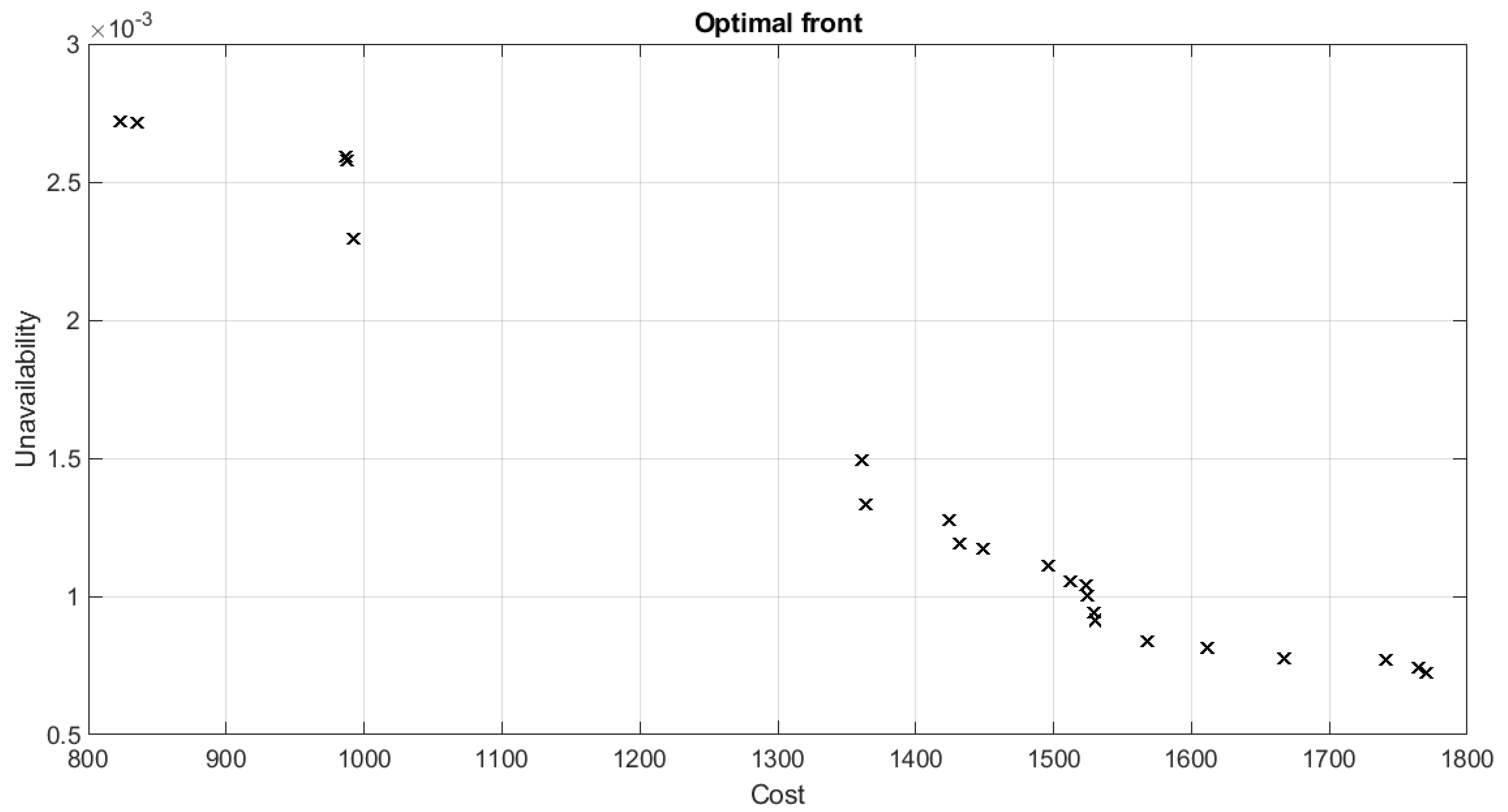
6.3. Accumulated Non-Dominated Set of Designs

The non-dominated solutions to the problem provided at the end of the evolutionary process for all executions, all configurations, all encodings and time units are shown in Figure 6. All optimum solutions belonging to the achieved non-dominated front are shown in Table 15. Unavailability ( Q ) is shown as a fraction, Cost is shown in economic units and the rest of the variables represent, for the respective devices, the optimum Time To Start a Preventive Maintenance activity with the hour, day or week as a time unit.
The solution with the lowest Cost (ID1) (823.38 economic units) represents the biggest Unavailability (0.002720). These values are followed by periodic optimum times (using the hour as a time unit in this case) measured from the moment in which the system mission time starts (Time To Perform a Preventive Maintenance activity ( T R P ) is not included). For solution ID1, it can be seen that periodic optimum Times To Start a Preventive Maintenance activity ( T P ) for devices P2 and V4 are not supplied. This is because the design alternative does not include such devices. The opposite case shows the biggest Cost (ID22) (1770.12 economic units) and the lowest Unavailability (0.000725). For solution ID22, periodic optimum Times To Start a Preventive Maintenance activity ( T P ) are supplied for all devices. This is because the design alternative includes devices P2 and V4. Other optimum solutions were found in these two solutions and can be seen in Table 15. The decision makers will need to decide which is the preferable design for them, taking into account their individual requirements.
Moreover, solutions were clustered in Figure 7 according to their final design. Solutions are shown from left to right and in ascending order in relation to the Cost from ID1 to ID22. The solutions contained in Cluster 1 (the solutions 1 to 2, see also Table 15) are the solutions in which non-redundant devices were included in the design. In this case, the system contains exclusively devices placed in series. These solutions present the lowest Cost and the biggest Unavailability. The solutions contained in Cluster 2 (the solutions 3 to 5, see also Table 15) are the solutions in which a redundant valve was included in the design as a parallel device. These solutions present a bigger Cost and a lower Unavailability than the solutions contained in Cluster 1. The solutions contained in Cluster 3 (the solutions 6 to 11, see also Table 15) are the solutions in which a redundant pump was included in the design as a parallel device. These solutions present a higher Cost and a lower Unavailability than the solutions contained in Clusters 1 and 2. Finally, the solutions contained in Cluster 4 (the solutions 12 to 22, see also Table 15) are the solutions in which both a redundant valve and a redundant pump were included in the design as parallel devices. These solutions present the biggest Cost and the lowest Unavailability.
The best accumulated non-dominated solutions obtained were used to compute the accumulated Hypervolume, whose value was 2.4651. As expected, the value is higher than the rest of the maximum accumulated values obtained after the evolutionary process for the encoding experiment and the accuracy experiment. This is shown in Table 16. This value is also higher than the value obtained in [6] and could be considered as an actual benchmark value of the case study.

7. Conclusions

In the present paper, a methodology presented previously by the authors [6] was used. This consists of coupling a Multi-Objective Evolutionary Algorithm and Discrete Simulation in order to optimise simultaneously both the system design (based on redundancy allocation) and its preventive maintenance strategy (based on determining periodic preventive maintenance activities with regard to each device included in the design), whilst addressing the conflict between Availability and operational Cost. The Multi-Objective Evolutionary Algorithm gives rise to a population of individuals, each encoding one design alternative and its preventive maintenance strategy. Each individual represents a possible solution to the problem, which is then used to modify and evaluate the system Functionability Profile through Discrete Simulation. The individuals evolve generation after generation until the stopping criterion is reached. This process was applied to a technical system in a case study in which two experiments were developed: Firstly, an encoding experiment which consisted of comparing the performance of seven encoding types (real, standard binary with one point, two point and uniform crossover, and Gray with one point, two point and uniform crossover), and secondly, an accuracy level encoding which consisted of comparing the performance of using standard binary encoding with accuracy levels across a range of time unit (hours, days and weeks) with impact in the form of size of the chromosome (the smaller the time unit, the bigger the chromosome). The Multi-objective Evolutionary Algorithm used was NSGA-II and a set of optimum non-dominated solutions were obtained for all cases.
In conclusion, the use of the Multi-Objective Evolutionary Algorithm NSGA-II and Discrete Simulation to address the joint optimisation of the system design and its preventive maintenance strategy provides Availability-Cost-balanced solutions to the real world problem studied, where data based on specific bibliography, mathematical relations and field experience were used. The computational cost reveals the complexity of the process and the necessity of using a computing cluster, which allowed parallel executions.
With regard to the encoding experiment, the best ordered method by the Friedman test case based on the final Hypervolume indicator distributions was the two point crossover standard binary encoding, although no statistically significant differences were observed. With regard to the accuracy experiment, the best ordered method by the Friedman test case based on the final Hypervolume indicator distributions was the two point crossover standard binary encoding with hours as a time unit, although no statistically significant differences were observed. From the authors’ point of view, an important conclusion arises from this experiment, which relates to flexibility regarding the time unit to schedule the preventive maintenance activities. Using the hour, the day or the week as a time unit does not affect significantly the performance of the configurations so, in the studied conditions, the preventive maintenance activities can be planned using weeks as a time unit. This allows a better range of time for planning than if days or hours are used as a time unit.
In addition, a higher benchmark value of the case study (in terms of Hypervolume indicator) is attained in this work as a reference.
As future work, the authors consider that these conclusions should be explored in greater depth extending the analysis to other real world problems in the reliability field, as well as comparing this analysis with other state of the art Multi-objective Evolutionary Algorithms.

Author Contributions

All of the authors contributed to publishing this article. Conceptualization A.C., D.G., B.J.G.; methodology, A.C., D.G., B.J.G.; software, A.C., D.G., B.J.G.; validation A.C., D.G., B.J.G.; formal analysis A.C., D.G., B.J.G.; investigation A.C., D.G., B.J.G.; resources D.G., B.J.G.; data curation, A.C., D.G., B.J.G.; writing—original draft preparation A.C., D.G.; writing—review and editing A.C., D.G., B.J.G.; visualization A.C., D.G., B.J.G.; supervision D.G., B.J.G.; funding acquisition D.G., B.J.G. All authors have read and agreed to the published version of the manuscript.

Funding

This research was funded by Pre-doctoral Research Staff of Universidad de Las Palmas de Gran Canaria (ULPGC) grant of Andrés Cacereño. The APC was funded by Instituto Universitario de Sistemas Inteligentes y Aplicaciones Numéricas en Ingeniería (SIANI) of ULPGC.

Institutional Review Board Statement

Not applicable.

Informed Consent Statement

Not applicable.

Data Availability Statement

Not applicable.

Acknowledgments

A. Cacereño is the recipient of a contract from the Program of Training for Pre-doctoral Research Staff of the University of Las Palmas de Gran Canaria. The authors are grateful for this support. We also convey our gratitude to MSc. Ernesto Primera, from the Machinery & Reliability Institute, Alabama, USA. David Greiner also acknowledges partial Project support funding from the Ministerio de Ciencia, Innovacion y Universidades, Gobierno de España, grant contract: PID2019-110185RB-C22, and from the Agencia Canaria de Investigacion, Innovacion y Sociedad de la Informacion, Consejeria de Economia, Conocimiento y Empleo del Gobierno de Canarias, Grant Contract Number: PROID2020010022, and European Regional Development Funds (ERDF/FEDER).

Conflicts of Interest

The authors declare no conflict of interest.

Appendix A. Detailed Information of the Case Study Parameters

  • Life Cycle. System mission time, expressed in hours.
  • Corrective Maintenance Cost. The cost involved in developing a repair activity to recover the system following a failure, expressed in economic units per hour.
  • Preventive Maintenance Cost. The cost involved in developing a Preventive Maintenance activity, expressed in relation to the Corrective Maintenance Cost.
  • Pump TF min . Minimum operation Time To Failure for a pump without Preventive Maintenance, expressed in hours.
  • Pump TF max . Maximum operation Time To Failure for a pump without Preventive Maintenance, expressed in hours.
  • Pump TF λ . Failure rate for a pump, which follows an exponential failure distribution, expressed in hours raised to the power of minus six.
  • Pump TR min . Minimum Time To Repair or duration of a Corrective Maintenance activity for a pump, expressed in hours.
  • Pump TR max . Maximum Time To Repair or duration of a Corrective Maintenance activity for a pump, expressed in hours.
  • Pump TR μ . Mean for the normal distribution followed for the Time To Repair assumed for a pump, expressed in hours.
  • Pump TR σ . Standard deviation for the normal distribution followed for the Time To Repair assumed for a pump, expressed in hours.
  • Pump TP min . Minimum operation Time To Start a scheduled Preventive Maintenance activity for a pump, expressed in hours.
  • Pump TP max . Maximum operation Time To Start a scheduled Preventive Maintenance activity for a pump, expressed in hours.
  • Pump TRP min . Minimum Time To Perform a Preventive Maintenance activity for a pump, expressed in hours.
  • Pump TRP max . Maximum Time To Perform a Preventive Maintenance activity for a pump, expressed in hours.
  • Valve TF min . Minimum operation Time To Failure for a valve without Preventive Maintenance, expressed in hours.
  • Valve TF max . Maximum operation Time To Failure for a valve without Preventive Maintenance, expressed in hours.
  • Valve TF λ . Failure rate for a valve, which follows an exponential failure distribution, expressed in hours raised to the power of minus six.
  • Valve TR min . Minimum Time To Repair or duration of a Corrective Maintenance activity for a valve, expressed in hours.
  • Valve TR max . Maximum Time To Repair or duration of a Corrective Maintenance activity for a valve, expressed in hours.
  • Valve TR μ . Mean for the normal distribution followed for the Time To Repair assumed for a valve, expressed in hours.
  • Valve TR σ . Standard deviation for the normal distribution followed for the Time To Repair assumed for a valve, expressed in hours.
  • Valve TP min . Minimum operation Time To Start a scheduled Preventive Maintenance activity for a valve, expressed in hours.
  • Valve TP max . Maximum operation Time To Start a scheduled Preventive Maintenance activity for a valve, expressed in hours.
  • Valve TRP min . Minimum Time To Perform a Preventive Maintenance activity for a valve, expressed in hours.
  • Valve TRP max . Maximum Time To Perform a Preventive Maintenance activity for a valve, expressed in hours.

References

  1. Misra, K.B. Reliability Engineering: A Perspective. In Handbook of Performability Engineering; Misra, K.B., Ed.; Springer Limited: London, UK, 2008; Chapter 19; pp. 253–289. ISBN 978-1-84800-130-5. [Google Scholar]
  2. Andrews, J.D.; Moss, T.R. Reliability and Risk Assessment, 2nd ed.; ASME Press: New York, NY, USA, 2002; p. 540. ISBN 0-7918-0183-7. [Google Scholar]
  3. Simon, D. Evolutionary Optimization Algorithms. Biologically Inspired and Population-Based Approaches to Computer Intelligence; John Wiley & Sons, Inc.: Hoboken, NJ, USA, 2013; p. 742. ISBN 978-0-470-93741-9. [Google Scholar]
  4. Kuo, W.; Prasad, R.; Tillman, F.A.; Mwang, C.L. Optimal Reliability Design: Fundamentals and Applications, 1st ed.; Cambridge University Press: Cambridge, UK, 2001; p. 389. ISBN 978-0-521-78127-5. [Google Scholar]
  5. Gao, Y.; Feng, Y.; Zhang, Z.; Tan, J. An optimal dynamic interval preventive maintenance scheduling for series systems. Reliab. Eng. Syst. Saf. 2015, 142, 19–30. [Google Scholar] [CrossRef]
  6. Cacereño, A.; Greiner, D.; Galván, B. Solving Multi-objective Optimal Design and Maintenance for Systems Based on Calendar Times Using NSGA-II. In Advances in Evolutionary and Deterministic Methods for Design, Optimization and Control in Engineering and Sciences; Gaspar-Cunha, A., Periaux, J., Giannakoglou, K.C., Gauger, N.R., Quagliarella, D., Greiner, D., Eds.; Springer Nature: Cham, Switzerland, 2021; pp. 245–259. [Google Scholar]
  7. Knezevic, J. Mantenibilidad, 1st ed.; Isdefe: Madrid, Spain, 1996; p. 209. ISBN 84-89338-08-6. [Google Scholar]
  8. Deb, K.; Pratap, A.; Agarwal, S.; Meyarivan, T. A Fast and Elitist Multiobjective Genetic Algorithm: NSGA-II. IEEE Trans. Evol. Comput. 2002, 6, 182–197. [Google Scholar] [CrossRef] [Green Version]
  9. Busacca, P.G.; Marseguerra, M.; Zio, E. Multiobjective optimization by genetic algorithms: Application to safety systems. Reliab. Eng. Syst. Saf. 2001, 72, 59–74. [Google Scholar] [CrossRef]
  10. Marseguerra, M.; Zio, E.; Podofillini, L.; Coit, D.W. Optimal Design of Reliable Network Systems in Presence of Uncertainty. IEEE Trans. Reliab. 2005, 54, 243–253. [Google Scholar] [CrossRef]
  11. Tian, Z.; Zuo, M.J. Redundancy allocation for multi-state systems using physical programming and genetic algorithms. Reliab. Eng. Syst. Saf. 2006, 91, 1049–1056. [Google Scholar] [CrossRef]
  12. Huang, H.Z.; Qu, J.; Zuo, M.J. Genetic-algorithm-based optimal apportionment of reliability and redundancy under multiple objectives. IIE Trans. 2009, 41, 287–298. [Google Scholar] [CrossRef]
  13. Zoulfaghari, H.; Hamadani, A.Z.; Ardakan, M.A. Bi-objective redundancy allocation problem for a system with mixed repairable and non-repairable components. ISA Trans. 2014, 53, 17–24. [Google Scholar] [CrossRef]
  14. Taboada, H.A.; Espiritu, J.F.; Coit, D.W. MOMS-GA: A Multi-Objective Multi-State Genetic Algorithm for System Reliability Optimization Design Problems. IEEE Trans. Reliab. 2008, 57, 182–191. [Google Scholar] [CrossRef]
  15. Taboada, H.A.; Baheranwala, F.; Coit, W.D.; Wattanapongsakorn, N. Practical solutions for multi-objective optimization: An application to system reliability design problems. Reliab. Eng. Syst. Saf. 2007, 92, 314–322. [Google Scholar] [CrossRef]
  16. Greiner, D.; Galván, B.; Winter, G. Safety Systems Optimum Design by Multicriteria Evolutionary Algorithms. In Evolutionary Multi-Criterion Optimization. Lecture Notes in Computer Science, Proceedings of the Second International Conference, EMO 2003, Faro, Portugal, 8–11 April 2003; Fonseca, C.M., Fleming, P.J., Zitzler, E., Deb, K., Thiele, L., Eds.; Springer: Berlin, Germany, 2003; pp. 722–736. [Google Scholar]
  17. Salazar, D.; Rocco, C.M.; Galván, B.J. Optimization of constrained multiple-objective reliability problems using evolutionary algorithms. Reliab. Eng. Syst. Saf. 2006, 91, 1057–1070. [Google Scholar] [CrossRef]
  18. Limbourg, P.; Kochs, H.D. Multi-objective optimization of generalized reliability design problems using feature models—A concept for early design stages. Reliab. Eng. Syst. Saf. 2008, 93, 815–828. [Google Scholar] [CrossRef]
  19. Kumar, R.; Izui, K.; Yoshimura, M.; Nishiwaki, S. Multi-objective hierarchical genetic algorithms for multilevel redundancy allocation optimization. Reliab. Eng. Syst. Saf. 2009, 94, 891–904. [Google Scholar] [CrossRef]
  20. Chambari, A.; Rahmati, S.H.A.; Najafi, A.A.; Karimi, A. A bi-objective model to optimize reliability and cost of system with a choice of redundancy strategies. Comput. Ind. Eng. 2012, 63, 109–119. [Google Scholar] [CrossRef]
  21. Safari, J. Multi-objective reliability optimization of series-parallel systems with a choice of redundancy strategies. Reliab. Eng. Syst. Saf. 2012, 108, 10–20. [Google Scholar] [CrossRef]
  22. Ardakan, M.A.; Hamadani, A.Z.; Alinaghian, M. Optimizing bi-objective redundancy allocation problem with a mixed redundancy strategy. ISA Trans. 2015, 55, 116–128. [Google Scholar] [CrossRef]
  23. Ghorabaee, M.K.; Amiri, M.; Azimi, P. Genetic algorithm for solving bi-objective redundancy allocation problem with k-out-of-n subsystems. Appl. Math. Model. 2015, 39, 6396–6409. [Google Scholar] [CrossRef]
  24. Amiri, M.; Khajeh, M. Developing a bi-objective optimization model for solving the availability allocation problem in repairable series–parallel systems by NSGA-II. J. Ind. Eng. Int. 2016, 12, 61–69. [Google Scholar] [CrossRef] [Green Version]
  25. Jahromi, A.E.; Feizabadi, M. Optimization of multi-objective redundancy allocation problem with non-homogeneous components. Comput. Ind. Eng. 2017, 108, 111–123. [Google Scholar] [CrossRef]
  26. Kayedpour, F.; Amiri, M.; Rafizadeh, M.; Nia, A.S. Multi-objective redundancy allocation problem for a system with repairable components considering instantaneous availability and strategy selection. Reliab. Eng. Syst. Saf. 2017, 160. [Google Scholar] [CrossRef]
  27. Sharifi, M.; Moghaddam, T.A.; Shahriari, M. Multi-objective Redundancy Allocation Problem with weighted-k-out-of-n subsystems. Heliyon 2019, 5, e02346. [Google Scholar] [CrossRef] [Green Version]
  28. Chambari, A.; Azimi, P.; Najafi, A.A. A bi-objective simulation-based optimization algorithm for redundancy allocation problem in series-parallel systems. Expert Syst. Appl. 2021, 173, 114745. [Google Scholar] [CrossRef]
  29. Zhao, J.H.; Liu, Z.; Dao, M.T. Reliability optimization using multiobjective ant colony system approaches. Reliab. Eng. Syst. Saf. 2007, 92, 109–120. [Google Scholar] [CrossRef]
  30. Chiang, C.H.; Chen, L.H. Availability allocation and multi-objective optimization for parallel–series systems. Eur. J. Oper. Res. 2007, 180, 1231–1244. [Google Scholar] [CrossRef]
  31. Elegbede, C.; Adjallah, K. Availability allocation to repairable systems with genetic algorithms: A multi-objective formulation. Reliab. Eng. Syst. Saf. 2003, 82, 319–330. [Google Scholar] [CrossRef]
  32. Khalili-Damghani, K.; Abtahi, A.R.; Tavana, M. A new multi-objective particle swarm optimization method for solving reliability redundancy allocation problems. Reliab. Eng. Syst. Saf. 2013, 111, 58–75. [Google Scholar] [CrossRef]
  33. Jiansheng, G.; Zutong, W.; Mingfa, Z.; Ying, W. Uncertain multiobjective redundancy allocation problem of repairable systems based on artificial bee colony algorithm. Chin. J. Aeronaut. 2014, 27, 1477–1487. [Google Scholar]
  34. Samanta, A.; Basu, K. An attraction based particle swarm optimization for solving multi-objective availability allocation problem under uncertain environment. J. Intell. Fuzzy Syst. 2018, 35, 1169–1178. [Google Scholar] [CrossRef]
  35. Muñoz, A.; Martorell, S.; Serradell, V. Genetic algorithms in optimizing surveillance and maintenance of components. Reliab. Eng. Syst. Saf. 1997, 57, 107–120. [Google Scholar] [CrossRef]
  36. Marseguerra, M.; Zio, E.; Podofillini, L. Condition-based maintenance optimization by means of genetic algorithms and Monte Carlo simulation. Reliab. Eng. Syst. Saf. 2002, 77, 151–166. [Google Scholar] [CrossRef]
  37. Gao, J.; Gen, M.; Sun, L. Scheduling jobs and maintenances in flexible job shop with a hybrid genetic algorithm. J. Intell. Manuf. 2006, 17, 493–507. [Google Scholar] [CrossRef]
  38. Sánchez, A.; Carlos, S.; Martorell, S.; Villanueva, J.F. Addressing imperfect maintenance modelling uncertainty in unavailability and cost based optimization. Reliab. Eng. Syst. Saf. 2009, 94, 22–32. [Google Scholar] [CrossRef]
  39. Wang, Y.; Pham, H. A multi-objective optimization of imperfect preventive maintenance policy for dependent competing risk systems with hidden failure. IEEE Trans. Reliab. 2011, 60, 770–781. [Google Scholar] [CrossRef]
  40. Ben Ali, M.; Sassi, M.; Gossab, M.; Harrath, Y. Simultaneous scheduling of production and maintenance tasks in the job shop. J. Intell. Manuf. 2011, 49. [Google Scholar] [CrossRef]
  41. An, Y.; Chen, X.; Zhang, J.; Li, Y. A hybrid multi-objective evolutionary algorithm to integrate optimization of the production scheduling and imperfect cutting tool maintenance considering total energy consumption. J. Clean Prod. 2020, 268, 121540. [Google Scholar] [CrossRef]
  42. Bressi, S.; Santos, J.; Losa, M. Optimization of maintenance strategies for railway track-bed considering probabilistic degradation models and different reliability levels. Reliab. Eng. Syst. Saf. 2021, 207, 107359. [Google Scholar] [CrossRef]
  43. Martorell, S.; Villanueva, J.F.; Carlos, S.; Nebot, Y.; Sánchez, A.; Pitarch, J.L.; Serradell, V. RAMS+C informed decision-making with application to multi-objective optimization of technical specifications and maintenance using genetic algorithms. Reliab. Eng. Syst. Saf. 2005, 87, 65–75. [Google Scholar] [CrossRef]
  44. Oyarbide-Zubillaga, A.; Goti, A.; Sanchez, A. Preventive maintenance optimisation of multi-equipment manufacturing systems by combining discrete event simulation and multi-objective evolutionary algorithms. Prod. Plan. Control. 2008, 19, 342–355. [Google Scholar] [CrossRef]
  45. Berrichi, A.; Amodeo, L.; Yalaoui, F.; Châtalet, E.; Mezghiche, M. Bi-objective optimization algorithms for joint production and maintenance scheduling: Application to the parallel machine problem. J. Intell. Manuf. 2009, 20, 389–400. [Google Scholar] [CrossRef]
  46. Moradi, E.; Fatemi Ghomi, S.M.T.; Zandieh, M. Bi-objective optimization research on integrated fixed time interval preventive maintenance and production for scheduling flexible job-shop problem. Expert Syst. Appl. 2011, 38, 7169–7178. [Google Scholar] [CrossRef]
  47. Hnaien, F.; Yalaoui, F. A bi-criteria flow-shop scheduling with preventive maintenance. IFAC Proc. Vol. 2013, 46, 1387–1392. [Google Scholar] [CrossRef]
  48. Wang, S.; Liu, M. Multi-objective optimization of parallel machine scheduling integrated with multi-resources preventive maintenance planning. J. Manuf. Syst. 2015, 37, 182–192. [Google Scholar] [CrossRef]
  49. Piasson, D.; Bíscaro, A.A.P.; Leão, F.B.; Sanches Mantovani, J.R. A new approach for reliability-centered maintenance programs in electric power distribution systems based on a multiobjective genetic algorithm. Electr. Power Syst. Res. 2016, 137, 41–50. [Google Scholar] [CrossRef] [Green Version]
  50. Sheikhalishahi, M.; Eskandari, N.; Mashayekhi, A.; Azadeh, A. Multi-objective open shop scheduling by considering human error and preventive maintenance. Appl. Math. Model. 2019, 67, 573–587. [Google Scholar] [CrossRef]
  51. Boufellouh, R.; Belkaid, F. Bi-objective optimization algorithms for joint production and maintenance scheduling under a global resource constraint: Application to the permutation flow shop problem. Comput. Oper. Res. 2020, 122, 104943. [Google Scholar] [CrossRef]
  52. Zhang, C.; Yang, T. Optimal maintenance planning and resource allocation for wind farms based on non-dominated sorting genetic algorithm-II. Renew. Energy 2021, 164, 1540–1549. [Google Scholar] [CrossRef]
  53. Berrichi, A.; Yalaoui, F.; Amodeo, L.; Mezghiche, M. Bi-Objective Ant Colony Optimization approach to optimize production and maintenance scheduling. Comput. Oper. Res. 2010, 37, 1584–1596. [Google Scholar] [CrossRef]
  54. Suresh, K.; Kumarappan, N. Hybrid improved binary particle swarm optimization approach for generation maintenance scheduling problem. Swarm Evol. Comput. 2013, 9, 69–89. [Google Scholar] [CrossRef]
  55. Li, J.Q.; Pan, Q.K.; Tasgetiren, M.F. A discrete artificial bee colony algorithm for the multi-objective flexible job-shop scheduling problem with maintenance activities. Swarm Evol. Comput. 2014, 38, 1111–1132. [Google Scholar] [CrossRef]
  56. Galván, B.; Winter, G.; Greiner, D.; Salazar, D.; Méndez, M. New Evolutionary Methodologies for Integrated Safety System Design and Maintenance Optimization. In Computational Intelligence in Reliability Engineering: Evolutionary Techniques in Reliability Analysis and Optimization; Levitin, G., Ed.; Springer: Berlin/Heidelberg, Germany, 2007; pp. 151–190. [Google Scholar]
  57. Okasha, N.M.; Frangopol, D.M. Lifetime-oriented multi-objective optimization of structural maintenance considering system reliability, redundancy and life-cycle cost using GA. Struct. Saf. 2009, 31, 460–474. [Google Scholar] [CrossRef]
  58. Adjoul, O.; Benfriha, K.; El Zant, C.; Aoussat, A. Algorithmic Strategy for Simultaneous Optimization of Design and Maintenance of Multi-Component Industrial Systems. Reliab. Eng. Syst. Saf. 2021, 208. [Google Scholar] [CrossRef]
  59. Lins, I.D.; Droguett, E.A.L. Multiobjective optimization of availability and cost in repairable systems design via genetic algorithms and discrete event simulation. Pesquisa Oper. 2009, 29, 43–66. [Google Scholar] [CrossRef] [Green Version]
  60. Lins, I.D.; López, E. Redundancy allocation problems considering systems with imperfect repairs using multi-objective genetic algorithms and discrete event simulation. Simul. Model. Pract. Theory 2011, 19, 362–381. [Google Scholar] [CrossRef]
  61. SINTEF. OREDA—Offshore Reliability Data Handbook, 5th ed.; Det Norske Veritas: Hovik, Norway, 2009; p. 796. ISBN 978-82-14-04830-8. [Google Scholar]
  62. Emmerich, M.; Deutz, A. A tutorial on multiobjective optimization: Fundamentals and evolutionary methods. Nat. Comput. 2018, 17, 585–609. [Google Scholar] [CrossRef] [Green Version]
  63. Coello, C.A. Multi-objective Evolutionary Algorithms in Real-World Applications: Some Recent Results and Current Challenges. In Advances in Evolutionary and Deterministic Methods for Design, Optimization and Control in Engineering and Sciences; Computational Methods in Applied Sciences; Greiner, D., Galván, B., Périaux, J., Gauger, N., Giannakoglou, K., Winter, G., Eds.; Springer International Publishing AG: Cham, Switzerland, 2015; pp. 3–18. [Google Scholar]
  64. Whitley, D.; Rana, S.; Heckendorn, R. Representation Issues in Neighborhood Search and Evolutionary Algorithms. In Genetic Algorithms and Evolution Strategies in Engineering and Computer Science; Quagliarella, D., Périaux, J., Poloni, C., Winter, G., Eds.; John Wiley & Sons: Chichester, UK, 1997; pp. 39–57. [Google Scholar]
  65. Savage, C. A Survey of Combinatorial Gray Codes. SIAM Rev. 1997, 39, 605–629. [Google Scholar] [CrossRef] [Green Version]
  66. Greiner, D.; Winter, G.; Emperador, J.M.; Galván, B. Gray Coding in Evolutionary Multicriteria Optimization: Application in Frame Structural Optimum Design. In Evolutionary Multi-Criterion Optimization. EMO 2005. Lecture Notes in Computer Science; Coello, C.A., Hernández Aguirre, A., Zitzler, E., Eds.; Springer: Berlin/Heidelberg, Germany, 2005; Volume 3410. [Google Scholar] [CrossRef]
  67. Tian, Y.; Cheng, R.; Zhang, X.; Jin, Y. PlatEMO: A MATLAB Platform for Evolutionary Multi-Objective Optimization [Educational Forum]. IEEE Comput. Intell. Mag. 2017, 12, 73–87. [Google Scholar] [CrossRef] [Green Version]
  68. Zitzler, E.; Thiele, L.; Laumanns, M.; Fonseca, C.M.; da Fonseca, V.G. Performance Assessment of Multiobjective Optimizers: An Analysis and Review. IEEE Trans. Evol. Comput. 2003, 7, 117–132. [Google Scholar] [CrossRef] [Green Version]
  69. Fonseca, C.M.; Paquete, L.; López-Ibáñez, M. An Improved Dimension-Sweep Algorithm for the Hypervolume Indicator. In Proceedings of the IEEE International Conference on Evolutionary Computation, Vancouver, BC, Canada, 16–21 July 2006; pp. 1157–1163. [Google Scholar] [CrossRef] [Green Version]
  70. Benavoli, A.; Corani, G.; Mangili, F. Should We Really Use Post-Hoc Tests Based on Mean-Ranks? J. Mach. Learn. Res. 2016, 17, 1–10. [Google Scholar]
Figure 1. Case study: fluid injection system.
Mathematics 09 01751 g001
Figure 2. Hypervolume Average vs. evaluations (encoding experiment).
Mathematics 09 01751 g002
Figure 3. Box plots of the final Hypervolume (encoding experiment).
Mathematics 09 01751 g003
Figure 4. Hypervolume Average vs. evaluations (accuracy experiment).
Mathematics 09 01751 g004
Figure 5. Box plots of the final Hypervolume (accuracy experiment).
Mathematics 09 01751 g005
Figure 6. Non-dominated front.
Mathematics 09 01751 g006
Figure 7. Design alternatives (encoding experiment).
Mathematics 09 01751 g007
Table 1. Data set for system devices.
ParameterValueSource
Life Cycle700,800 h-
Corrective Maintenance Cost0.5 unitsMachinery & Reliability Institute
Preventive Maintenance Cost0.125 unitsMachinery & Reliability Institute
Pump T F m i n 1 hMachinery & Reliability Institute
Pump T F m a x 70,080 hMachinery & Reliability Institute
Pump T F   λ 159.57 × 10 6 hOREDA 2009
Pump T R m i n 1 hMachinery & Reliability Institute
Pump T R m a x 24.33 h μ + 4 σ
Pump T R   μ 11 hOREDA 2009
Pump T R   σ 3.33 h( μ – TRmin)/3
Pump T P m i n 2920 hMachinery & Reliability Institute
Pump T P m a x 8760 hMachinery & Reliability Institute
Pump T R P m i n 4 hMachinery & Reliability Institute
Pump T R P m a x 8 hMachinery & Reliability Institute
Valve T F m i n 1 hMachinery & Reliability Institute
Valve T F m a x 70,080 hMachinery & Reliability Institute
Valve T F   λ 44.61 × 10 6 hOREDA 2009
Valve T R m i n 1 hMachinery & Reliability Institute
Valve T R m a x 20.83 h μ + 4 σ
Valve T R   μ 9.5 hOREDA 2009
Valve T R   σ 2.83 h( μ – TRmin)/3
Valve T P m i n 8760 hMachinery & Reliability Institute
Valve T P m a x 35,040 hMachinery & Reliability Institute
Valve T R P m i n 1 hMachinery & Reliability Institute
Valve T R P m a x 3 hMachinery & Reliability Institute
Table 2. Parameters to configure the evolutionary process.
MethodEncodingCrossoverTime UnitPopulationPrMdisMPrCdisC
NSGA-IIRealSBXHour50-100-1500.5-1-1.520120
Standard Binary1 point (1PX)Hour50-100-1500.5-1-1.5-1-
Standard Binary2 Point (2PX)Hour50-100-1500.5-1-1.5-1-
Standard BinaryUniform (UX)Hour50-100-1500.5-1-1.5-1-
Gray1 Point (1PX)Hour50-100-1500.5-1-1.5-1-
Gray2 Point (2PX)Hour50-100-1500.5-1-1.5-1-
GrayUniform (UX)Hour50-100-1500.5-1-1.5-1-
Standard Binary1 Point (1PX)Day50-100-1500.5-1-1.5-1-
Standard Binary2 Point (2PX)Day50-100-1500.5-1-1.5-1-
Standard BinaryUniform (UX)Day50-100-1500.5-1-1.5-1-
Standard Binary1 Point (1PX)Week50-100-1500.5-1-1.5-1-
Standard Binary2 Point (2PX)Week50-100-1500.5-1-1.5-1-
Standard BinaryUniform (UX)Week50-100-1500.5-1-1.5-1-
Table 3. Computational time consumed.
EncodingTime UnitAverage TimeSequential Time
Real SBXHour2 days, 18 h and 12 min.8 months, 4 days, 23 h and 22 min.
Binary 1PXHour2 days, 18 h and 57 min.8 months, 7 days, 18 h and 48 min.
Binary 2PXHour3 days, 2 h and 39 min.9 months, 6 days, 5 h and 52 min.
Binary UXHour3 days and 39 min.8 months, 29 days, 3 h and 8 min.
Gray 1PXHour2 days, 19 h and 35 min.8 months, 10 days, 3 h and 23 min.
Gray 2PXHour2 days, 19 h and 56 min.8 months, 11 days, 11 h and 29 min.
Gray UXHour2 days, 19 h and 40 min.8 months, 10 days, 10 h and 34 min.
Total 2 days, 21 h and 6 min.4 years, 11 months, 19 days, 8 h and 36 min.
Table 4. Hypervolume statistics (Real encoding).
IdentifierConfigurationAverageMedianMax.Min.St. D.Friedman’s Test
Av. Rank
ID1N = 50; PrM = 0.52.28212.28572.30792.25310.01795.900
ID2N = 100; PrM = 0.52.28862.28312.32582.26820.01704.800
ID3N = 150; PrM = 0.52.29382.28832.31872.27300.01444.300
ID4N = 50; PrM = 12.29272.29322.31132.27100.01173.999
ID5N = 100; PrM = 12.28632.29162.30642.25840.01485.200
ID6N = 150; PrM = 12.28902.28852.31572.26190.01705.100
ID7N = 50; PrM = 1.52.28572.27882.32282.27010.01716.100
ID8N = 100; PrM = 1.52.28212.28262.30512.25610.01625.600
ID9N = 150; PrM = 1.52.29682.29622.33072.26410.02114.000
p-value 0.5788
Table 5. Hypervolume statistics (Binary encoding).
EncodingIdentifierConfigurationAverageMedianMax.Min.St. D.Friedman’s Test
Av. Rank
B1PXID1N = 50; PrM = 0.52.29362.29192.32972.27380.01694.600
ID2N = 100; PrM = 0.52.29192.29532.30572.27030.01074.500
ID3N = 150; PrM = 0.52.28632.29152.29842.25540.01325.400
ID4N = 50; PrM = 12.29292.29182.31512.25660.01714.400
ID5N = 100; PrM = 12.28652.28222.32002.26740.01515.799
ID6N = 150; PrM = 12.29322.29262.32162.27610.01504.700
ID7N = 50; PrM = 1.52.28032.27752.29942.26420.01367.000
ID8N = 100; PrM = 1.52.29702.30082.31262.27080.01343.100
ID9N = 150; PrM = 1.52.28842.28712.33942.26160.02095.500
p-value 0.1228
B2PXID1N = 50; PrM = 0.52.28082.28002.31732.24010.02376.500
ID2N = 100; PrM = 0.52.30132.30512.32602.27140.01723.300
ID3N = 150; PrM = 0.52.29162.28752.36272.26300.02985.400
ID4N = 50; PrM = 12.29412.29262.31562.27240.01524.600
ID5N = 100; PrM = 12.29082.29292.30562.27550.00894.800
ID6N = 150; PrM = 12.29212.29052.32152.26440.01604.999
ID7N = 50; PrM = 1.52.29242.28732.34832.26940.02265.100
ID8N = 100; PrM = 1.52.29312.29302.33262.26060.02054.900
ID9N = 150; PrM = 1.52.28832.28492.31072.27380.01455.399
p-value 0.4762
BUXID1N = 50; PrM = 0.52.28412.28282.30232.26110.01225.500
ID2N = 100; PrM = 0.52.29542.30002.31412.26470.01633.300
ID3N = 150; PrM = 0.52.28832.28802.32652.25760.01995.200
ID4N = 50; PrM = 12.29592.29392.34972.27020.02233.400
ID5N = 100; PrM = 12.28482.28662.30462.26600.01405.700
ID6N = 150; PrM = 12.28302.28502.29552.26870.00855.799
ID7N = 50; PrM = 1.52.28932.28662.31122.26220.01635.100
ID8N = 100; PrM = 1.52.28082.28002.29942.25790.01386.100
ID9N = 150; PrM = 1.52.28572.28552.30362.26570.01214.899
p-value 0.2132
Table 6. Hypervolume Statistics (Gray Encoding).
EncodingIdentifierConfigurationAverageMedianMax.Min.St. D.Friedman’s Test
Av. Rank
G1PXID1N = 50; PrM = 0.52.28332.28382.29292.27100.00645.500
ID2N = 100; PrM = 0.52.29902.30102.35562.26400.02523.600
ID3N = 150; PrM = 0.52.28152.28502.29512.26260.00996.200
ID4N = 50; PrM = 12.28652.28342.30172.27620.00835.200
ID5N = 100; PrM = 12.29892.29862.33472.26520.01863.100
ID6N = 150; PrM = 12.28122.27912.30432.26110.01176.000
ID7N = 50; PrM = 1.52.28822.29162.31712.25260.01874.200
ID8N = 100; PrM = 1.52.27862.28042.29922.26080.01376.100
ID9N = 150; PrM = 1.52.28742.28202.31802.27060.01555.100
p-value 0.0943
G2PXID1N = 50; PrM = 0.52.29472.29712.31922.27570.01283.700
ID2N = 100; PrM = 0.52.28022.28142.29532.25920.01216.500
ID3N = 150; PrM = 0.52.28562.28952.29782.25190.01364.299
ID4N = 50; PrM = 12.29122.28682.31862.26590.01924.900
ID5N = 100; PrM = 12.28322.28352.29512.26900.00705.600
ID6N = 150; PrM = 12.28992.29132.32562.26400.01934.100
ID7N = 50; PrM = 1.52.28662.28802.31322.26170.01694.800
ID8N = 100; PrM = 1.52.28092.28132.31402.25850.01486.500
ID9N = 150; PrM = 1.52.29202.29122.33642.27390.01694.600
p-value 0.2164
GUXID1N = 50; PrM = 0.52.28622.28922.30882.25400.01804.300
ID2N = 100; PrM = 0.52.28282.28132.29672.26960.00795.100
ID3N = 150; PrM = 0.52.28852.29222.30772.26660.01364.100
ID4N = 50; PrM = 12.29072.29392.31342.26830.01564.000
ID5N = 100; PrM = 12.28792.28582.31652.26110.01874.699
ID6N = 150; PrM = 12.28352.28162.30482.27010.01205.400
ID7N = 50; PrM = 1.52.28622.28522.30562.26080.01435.600
ID8N = 100; PrM = 1.52.28522.28512.30682.25240.01535.100
ID9N = 150; PrM = 1.52.27552.27002.30642.26380.01426.700
p-value 0.4572
Table 7. Hypervolume statistics (Encoding experiment).
IdentifierDescriptionConfigurationAverageMedianMax.Min.St. D.Friedman’s Test
Av. Rank
ID1RealN = 50; PrM = 12.29272.29322.31132.27100.01174.600
ID2Binary 1PN = 100; PrM = 1.52.29702.30082.31262.27080.01344.000
ID3Binary 2PN = 100; PrM = 0.52.30132.30512.32602.27140.01723.000
ID4Binary UN = 100; PrM = 0.52.29542.30002.31412.26470.01634.199
ID5Gray 1PN = 100; PrM = 12.29892.29862.33472.26520.01863.500
ID6Gray 2PN = 50; PrM = 0.52.29472.29712.31922.27570.01284.000
ID7Gray UN = 50; PrM = 12.29072.29392.31342.26830.01564.699
p-value 0.5979
Table 8. Maximum accumulated Hypervolume value (encoding experiment).
EncodingHypervolume Accumulated Value
Real2.3943
Binary 1 Point Crossover2.4142
Binary 2 Point Crossover2.4298
Binary Uniform Crossover2.3984
Gray 1 Point Crossover2.4011
Gray 2 Point Crossover2.3982
Gray Uniform Crossover2.3829
Global2.4553
Table 9. Computational time consumed.
EncodingTime UnitAverage TimeSequential Time
Binary 1PXHour2 days, 18 h and 57 min8 months, 7 days, 18 h and 48 min.
Binary 2PXHour3 days, 2 h and 39 min9 months, 6 days, 5 h and 52 min.
Binary UXHour3 days and 39 min8 months, 29 days, 3 h and 8 min.
Binary 1PXDay2 days, 22 h and 3 min8 months, 19 days, 9 h and 14 min.
Binary 2PXDay2 days, 19 h and 13 min8 months, 8 days, 18 h and 18 min.
Binary UXDay2 days, 19 h and 13 min8 months, 8 days, 18 h and 55 min.
Binary 1PXWeek2 days, 18 h and 3 min8 months, 4 days, 9 h and 39 min.
Binary 2PXWeek2 days, 19 h and 21 min8 months, 9 days, 6 h and 55 min.
Binary UXWeek2 days, 19 h and 20 min8 months, 9 days, 4 h and 40 min.
Total 2 days, 20 h and 53 min6 years, 4 months, 12 days, 22 h and 41 min.
Table 10. Hypervolume statistics (Binary encoding-Days).
EncodingIdentifierConfigurationAverageMedianMax.Min.St. D.Friedman’s Test
Av. Rank
B1PX-DID1N = 50; PrM = 0.52.28342.27812.34302.26550.02205.800
ID2N = 100; PrM = 0.52.29422.29112.31982.27880.01334.100
ID3N = 150; PrM = 0.52.27852.28342.29342.25630.01266.600
ID4N = 50; PrM = 12.28192.27952.31272.26220.01525.800
ID5N = 100; PrM = 12.28962.28702.31882.26210.01844.500
ID6N = 150; PrM = 12.29642.29412.31932.28040.01033.200
ID7N = 50; PrM = 1.52.29222.29322.32392.27070.01774.400
ID8N = 100; PrM = 1.52.27762.27932.30572.25300.01716.800
ID9N = 150; PrM = 1.52.29392.29472.31072.27580.01353.800
p-value 0.0246
B2PX-DID1N = 50; PrM = 0.52.28382.27952.30432.26810.01235.400
ID2N = 100; PrM = 0.52.27832.27852.29472.26090.01066.600
ID3N = 150; PrM = 0.52.28672.28802.30432.27570.00844.300
ID4N = 50; PrM = 12.29302.28652.31732.27460.01764.200
ID5N = 100; PrM = 12.28742.28312.31882.26520.01925.399
ID6N = 150; PrM = 12.29162.29372.31502.27120.01524.100
ID7N = 50; PrM = 1.52.28772.28492.32492.26930.01614.600
ID8N = 100; PrM = 1.52.28412.28172.31362.26580.01335.300
ID9N = 150; PrM = 1.52.28872.28262.33722.26510.02165.100
p-value 0.5612
BUX-DID1N = 50; PrM = 0.52.29182.29482.31522.26430.01684.200
ID2N = 100; PrM = 0.52.28972.28652.33562.26020.01984.699
ID3N = 150; PrM = 0.52.28442.28662.31042.25220.01795.600
ID4N = 50; PrM = 12.27982.27322.30782.26010.01606.400
ID5N = 100; PrM = 12.28972.28932.31272.27290.01514.800
ID6N = 150; PrM = 12.29232.29072.33332.26660.02194.700
ID7N = 50; PrM = 1.52.28942.28802.32012.26910.01385.100
ID8N = 100; PrM = 1.52.29232.29012.32792.26370.01835.000
ID9N = 150; PrM = 1.52.29082.28632.34612.26060.02494.500
p-value 0.8007
Table 11. p-values from Wilcoxon signed-rank test.
Comparisonp-ValueConclusion
ID3 versus ID60.0059Significant difference found
ID4 versus ID60.0371Significant difference found
ID6 versus ID80.0371Significant difference found
ID1 versus ID60.0840The null hypothesis cannot be rejected
ID5 versus ID60.3223The null hypothesis cannot be rejected
ID2 versus ID60.3750The null hypothesis cannot be rejected
ID6 versus ID70.4922The null hypothesis cannot be rejected
ID6 versus ID90.6250The null hypothesis cannot be rejected
Table 12. Hypervolume statistics (Binary encoding-Weeks).
EncodingIdentifierConfigurationAverageMedianMax.Min.St. D.Friedman’s Test
Av. Rank
B1PX-WID1N = 50; PrM = 0.52.29572.29352.34302.25610.02504.300
ID2N = 100; PrM = 0.52.28722.28732.31272.26650.01425.100
ID3N = 150; PrM = 0.52.28972.28082.32522.26230.02125.100
ID4N = 50; PrM = 12.28122.28052.29772.25200.01575.799
ID5N = 100; PrM = 12.29072.28932.30072.28120.00603.999
ID6N = 150; PrM = 12.28252.28252.30042.26790.01016.100
ID7N = 50; PrM = 1.52.28902.28992.31102.25970.01644.900
ID8N = 100; PrM = 1.52.28742.28482.30662.26900.01235.000
ID9N = 150; PrM = 1.52.28882.28922.31762.26340.01554.700
p-value 0.7979
B2PX-WID1N = 50; PrM = 0.52.29172.29112.31012.27640.01214.000
ID2N = 100; PrM = 0.52.28582.28582.30132.26710.01225.300
ID3N = 150; PrM = 0.52.28922.28692.32372.25670.02504.900
ID4N = 50; PrM = 12.27972.27432.30142.27030.01086.299
ID5N = 100; PrM = 12.28402.28382.29652.26650.00855.200
ID6N = 150; PrM = 12.27932.27802.30662.25020.01476.200
ID7N = 50; PrM = 1.52.29212.28172.34652.27090.02464.899
ID8N = 100; PrM = 1.52.28952.28802.31982.25460.01684.001
ID9N = 150; PrM = 1.52.29182.28542.31302.27100.01454.200
p-value 0.4439
BUX-WID1N = 50; PrM = 0.52.28942.28472.33362.26590.01975.500
ID2N = 100; PrM = 0.52.29252.29222.31442.27560.01134.399
ID3N = 150; PrM = 0.52.29112.29322.32162.26640.01564.399
ID4N = 50; PrM = 12.28582.28362.30572.26600.01285.499
ID5N = 100; PrM = 12.28262.28342.31442.26310.01406.700
ID6N = 150; PrM = 12.28542.28572.31222.26450.01645.499
ID7N = 50; PrM = 1.52.28932.28872.30942.26810.01254.899
ID8N = 100; PrM = 1.52.30092.29422.33162.28700.01453.400
ID9N = 150; PrM = 1.52.29212.28622.31632.27740.01434.700
p-value 0.3128
Table 13. Hypervolume statistics (accuracy experiment).
Id.DescriptionConfigurationAverageMedianMax.Min.St. D.Friedman’s Test
Av. Rank
ID1Binary 1P (hour)N = 100; PrM = 1.52.29702.30082.31262.27080.01344.700
ID2Binary 2P (hour)N = 100; PrM = 0.52.30132.30512.32602.27140.01723.699
ID3Binary U (hour)N = 100; PrM = 0.52.29542.30002.31412.26470.01634.500
ID4Binary 1P (day)N = 150; PrM = 1.02.29642.29412.31932.28040.01035.000
ID5Binary 2P (day)N = 150; PrM = 1.02.29162.29372.31502.27120.01525.800
ID6Binary U (day)N = 50; PrM = 0.52.29182.29482.31522.26430.01685.300
ID7Binary 1P (week)N = 100; PrM = 1.02.29072.28932.30072.28120.00606.200
ID8Binary 2P (week)N = 50; PrM = 0.52.29172.29112.31012.27640.01215.900
ID9Binary U (week)N = 100; PrM = 1.52.30092.29422.33162.28700.01453.900
p-value 0.4053
Table 14. Maximum accumulated Hypervolume value (accuracy experiment).
EncodingTime UnitHypervolume Accumulated Value
Binary 1 Point CrossoverHour2.4142
Binary 2 Point CrossoverHour2.4298
Binary Uniform CrossoverHour2.3984
Binary 1 Point CrossoverDay2.4007
Binary 2 Point CrossoverDay2.3942
Binary Uniform CrossoverDay2.3984
Binary 1 Point CrossoverWeek2.4047
Binary 2 Point CrossoverWeek2.4285
Binary Uniform CrossoverWeek2.4037
Global 2.4646
Table 15. Optimum solutions (encoding experiment).
IdQCost [eu]Time UnitV1 [h]P2 [h]P3 [h]V4 [h]V5 [h]V6 [h]V7 [h]
10.002720823.38Hours25,40808633034,17934,90331,386
20.002713835.75Hours29,22508633027,07033,45433,690
30.002591986.88Days1285035390214419671386
40.002576988.00Weeks127047165206172203
50.002295992.75Days14350350830108814591454
60.0014951360.50Hours34,74682398408032,67631,76931,484
70.0013341363.75Days13943603150112513011026
80.0012761424.25Weeks20450370174173188
90.0011891431.75Hours31,04086178103034,78731,44529,929
100.0011741449.00Days17851500182171195
110.0011121496.12Weeks11248480176196144
120.0010561512.50Days8803583541186102013461098
130.0010391524.00Weeks1624542195147176189
140.0010021524.62Hours28,0427228654930,77720,95131,77934,982
150.0009391528.88Hours29,9397028790421,69025,71134,81434,791
160.0009131530.38Weeks1944749103137145179
170.0008351567.75Days1028363340128014309861326
180.0008131611.38Hours22,5165955629817,23729,56827,07522,757
190.0007761667.25Hours32,3557185838427,48926,94932,70032,770
200.0007711741.00Hours27,4437556852030,00330,05630,57921,639
210.0007421764.75Hours22,7768696850612,25634,76333,00629,706
220.0007251770.12Hours30,8137371845329,95816,34530,77625,358
Table 16. Maximum accumulated Hypervolume value.
ExperimentHypervolume Accumulated Value
Encoding2.4553
Accuracy2.4646
Total2.4651
Publisher’s Note: MDPI stays neutral with regard to jurisdictional claims in published maps and institutional affiliations.

