Design of Optimal Controllers for Unknown Dynamic Systems through the Nelder–Mead Simplex Method

Abstract

This paper presents an efficient method for designing optimal controllers. First, we established a performance index according to the system characteristics. In order to ensure that this performance index is applicable even when the state/output of the system is not within the allowable range, we added a penalty function. When we use a certain controller, if the state/output of the system remains within the allowable range within the preset time interval, the penalty function value is zero. Conversely, if the system state/output is not within the allowable range before the preset termination time, the experiment/simulation is terminated immediately, and the penalty function value is proportional to the time difference between the preset termination time and the time at which the experiment was terminated. Then, we used the Nelder–Mead simplex method to search for the optimal controller parameters. The proposed method has the following advantages: (1) the dynamic equation of the system need not be known; (2) the method can be used regardless of the stability of the open-loop system; (3) this method can be used in nonlinear systems; (4) this method can be used in systems with measurement noise; and (5) the method can improve design efficiency.

1. Introduction

In the real world, all dynamic systems are nonlinear; linear systems exist only in theory. Many methods of analysis and control have been proposed for nonlinear systems [1,2]. Among these, Lyapunov’s method can not only be used to analyze the stability of nonlinear systems; it is also often used to design feedback controllers. At present, many nonlinear control techniques based on Lyapunov theory have been proposed and applied to actual physical systems, such as Lyapunov redesign, backstepping, adaptive control, sliding mode control, etc. The recent developments and applications of the above methods are as follows.

Tavasoli and Enjilela utilized Lyapunov redesign to stabilize the vibration of a boundary-controlled flexible rectangular plate in the presence of exogenous disturbances [3]. Xu et al., applied output-feedback Lyapunov redesign to control a magnetic suspension system [4]. A backstepping controller was applied to control a quadrotor unmanned aerial vehicle [5], microgyroscope [6], and multiphase motor drives [7]. Adaptive control is a control method that can adapt to parameter changes or initially uncertain controlled systems. Recently, Liu et al., developed a novel adaptive fault-tolerant control strategy to suppress the vibrations of a flexible panel [8]. Liang et al., proposed neural-network-based event-triggered adaptive control for nonaffine nonlinear multiagent systems with dynamic uncertainties [9]. Wang and Na presented parameter estimation and adaptive control for servo mechanisms with friction compensation [10]. Since the publication of the survey paper on sliding mode control in IEEE Transactions of Automatic Control in 1977 [11], sliding mode control has been extensively studied and used in practical applications due to its simplicity and robustness with respect to external disturbances and modeling uncertainties [12,13,14]. In addition, gain scheduling is used to design corresponding linear controllers for nonlinear systems at different operating points or regions [15,16]. Feedback linearization is based on the theory of differential geometry to find an appropriate conversion between the control input and state variables and to convert the nonlinear system into an equivalent linear system. This method has been used for induction motors [17], boost converters [18], an unmanned bicycle robot [19], etc.

However, these methods usually require information on the approximate/nominal dynamic equation of the system and the upper bound of uncertainty or disturbance. Moreover, real controllers are always limited in magnitude. Therefore, in the actual design of a controller, we usually adopt a trial-and-error method. However, during adjustment of the parameters, the state or output of the system may not be within the allowable range. When this occurs, the experiment must be immediately terminated and relevant safety or protective measures must be initiated to prevent injury to the operator or damage to equipment. Therefore, designing a controller with good performance for real applications is difficult and time consuming.

To overcome the aforementioned difficulties and complexity associated with designing actual controllers, we propose an efficient and optimized controller design method for nonlinear unstable systems. First, we establish a performance index (objective function) according to the characteristics of the system to be controlled. This performance index may include a time function and any measurable system state or output signal; the dynamic equation of the system need not be known in advance. Moreover, the performance index itself or the dynamic equation of the system can also contain non-differentiable terms. Most importantly, to ensure that the performance index is applicable even when the state or output of the system is not within the allowable range, we add a special penalty function. The penalty function is used to solve constrained optimization problems. It is used to convert constrained problems into unconstrained problems by introducing an artificial penalty for violating the constraint.

The implication of the penalty function proposed in this paper is as follows. We assume that for the same system, the time interval between the beginning and termination of each experiment or simulation is fixed. When we use a certain set of controller parameters to control the system, if the state or output of the system is within the allowable range within the preset termination time, the penalty function value is zero. Conversely, if the system state or output is not within the allowable range before the preset termination time, the experiment or simulation is terminated immediately, and the penalty function value is proportional to the time difference between the preset termination time and the time at which the experiment was terminated.

To keep the performance index as low as possible, we used the Nelder–Mead (N–M) simplex method (also known as the downhill simplex method) to search for controller parameters. The original concept of the N–M simplex method was proposed by Spendley, Hext, and Himsworth [20], and it was further improved by Nelder and Mead [21]. The convergence properties of the Nelder-Mead simplex method are discussed in references [22,23,24,25]. Because the N–M simplex method is easy to implement, it has been widely used to search for the minimum or maximum value of the objective function in a multidimensional parameter space. In particular, the N–M simplex method does not require the derivative of the objective function; therefore, the real system is applicable even if it has nondifferentiable problems or the objective function value contains noise. The N–M simplex method continues to be applied in different fields, such as parameter estimation [26,27], optimization of machining parameters [28], power plant optimization [29], optimization of the production parameters for bread rolls [30], etc.

To verify the feasibility of the proposed method, we adopted an inverted pendulum system with measurement noise as an example. Then, we employed the N–M simplex method to search for the controller parameters iteratively. The simulation results revealed that even if the initial controller parameters cannot stabilize the system, after the algorithm reaches the iterative termination condition we set in advance, the system is stable and exhibits good transient response performance.

2. Design of Optimal Controllers for Unknown Parameter Systems

Optimal control is a branch of optimization problems that deals with finding a controller for a dynamical system over a period of time such that an objective function is optimized [31,32]. An objective function is usually called a performance index in the field of control. The purpose of optimization is to obtain a parameter vector such that the objective function is at a minimum. However, in many cases, the choice of parameters is not arbitrary but subject to certain restrictive conditions. We term this the constrained optimization problem. A general constrained minimization problem may be written as follows:

$$\min J(p)$$

(1)

$$\mathrm{subject} \mathrm{to} g_i\left(p\right)\le 0, i=1,2,\dots ,m_1$$

$$h_j\left(p\right)=0, j=1,2,\dots ,m_2$$

For a constrained optimization problem, we usually convert the constraints into a suitable penalty function and add this function to the original objective function. Thus, we transform a constrained optimization problem into an unconstrained problem; moreover, the solution of the unconstrained problem converges to the solution of the original constrained problem.

In the field of optimization control, the commonly used performance indices are as follows [31,32,33]:

• Integral squared error (ISE):

  $$J={\displaystyle {\int }_0^{T_f}{e}^2(t)} dt$$

  (2)

  The smaller the value of this index, the closer the error of the control system in the time interval [0, $T_f$] is to zero.
• Integral absolute error (IAE):

  $$J={\displaystyle {\int }_0^{T_f}\left|e(t)\right|} dt$$

  (3)

  The meaning of this index is similar to that of the ISE.
• Integral time-weighted absolute error (ITAE):

  $$J={\displaystyle {\int }_0^{T_f}t\left|e(t)\right|} dt$$

  (4)

  The smaller the value of this index, the closer the error of the control system in the time interval [0, $T_f$] to zero and the faster the convergence.
• Integral time-squared error (ITSE):

  $$J={\displaystyle {\int }_0^{T_f}t{e}^2(t)} dt$$

  (5)

  The meaning of this index is similar to that of the ITAE.
• Quadratic performance index:

  $$J=x^T(T_f)F(T_f)x(T_f)+{\displaystyle {\int }_0^{T_f}\left(x^{T}Qx+u^{T}Ru\right)} dt$$

  (6)

  where $T_f$, $e$, $x={[\begin{array}{cccc}{x}_1& x_2& \cdots & x_n\end{array}]}^T$, and $u={[\begin{array}{cccc}{u}_1& u_2& \cdots & u_{m_u}\end{array}]}^T$ denote the terminal time, output error, system state, and control input, respectively. Additionally, $F$ and $Q$ are positive semidefinite matrices, and $R$ is a positive definite matrix. When the control objective is to keep the state small, the control input not too large, and the final state as close to zero as possible, we can use this performance index.

The method proposed in this study does not require information on the dynamic equation of the system in advance, and it can use any of the above performance indices or other suitable performance indices. To ensure that the selected performance index is applicable even when the state or output of the system is not within the allowable range, we add a penalty function to the performance index. Before formally defining the penalty function, we first assume that, for the same system, the start time of each experiment (or simulation) is zero, and the terminal time is fixed and represented by $T_f$. If the state or output of the system is within the allowable variation range until the terminal time is reached, the penalty function weight $W_r$ is equal to zero. Conversely, if the state or output leaves the allowable variation range before reaching the terminal time, the experiment (or simulation) is terminated immediately; we denote this instant as $T_r$, and we then let the penalty function weight $W_r$ be a sufficiently large positive constant. Then, we define the penalty function as follows:

$$P=W_r\left(T_f-T_r\right)$$

(7)

To design controller parameters such that the performance index reaches the minimum value, we use the N–M simplex method to search for the controller parameters.

The N–M simplex method proposed by Nelder and Mead [21] is used for solving N-dimensional unconstrained optimization problems of the following form:

$$\underset{p\in {ℝ}^N}{\min }J(p)$$

(8)

where $J(p)$ is defined as an objective function, which is usually called the performance index in the control field.

After the form of the performance index is determined, the N–M simplex method generates a sequence of simplices, where each simplex is defined by $N+1$ distinct vertices, namely, $p_0,\dots ,p_N$, for which the corresponding function values are $J_0, \dots , J_N$. The points $p_0,\dots ,p_N$ are assumed to be sorted such that $J_0\le \cdots \le J_{N-1}<J_N$, and $\overline{p}$ represents the centroid of points $p_0,\dots ,p_{N-1}$. In each iteration, simplex transformations in the N–M simplex method are controlled by the parameters $\alpha$, $\beta$, and $\gamma$. These parameters should satisfy the following conditions:

$$0<\beta <1, 0<\alpha <\gamma$$

(9)

These parameters have typical values of $\alpha =1$, $\beta =0.5$, and $\gamma =2$. The values of $\alpha$, $\gamma$, $\beta$, and $-\beta$ yield the reflection point $p_r$, expansion point $p_e$, outer contraction point $p_c$, and inner contraction point $p_{cc}$, respectively. The objection functions at these four points are denoted as $J_r$, $J_e$, $J_c$, and $J_{cc}$, respectively. If none of the four points represents an improvement in the current worst point $p_N$, the algorithm shrinks the points $p_1,\dots ,p_N$ toward the lowest $p_0$, thereby producing a new simplex. During the shrinking process, each value of $p_i$ is replaced by $p_0+0.5\left(p_i-p_0\right)$ for $i=1,\dots ,N$. A new iteration is automatically triggered after the shrinking process is complete. The iterative process continues until the specified termination criteria are satisfied (e.g., the iterations reach the allowed maximum number or the function value $J_0$ is lower than the default value). We list the various vertices that may be tried during the iteration of the N–M simplex method in Table 1. The pseudo code of the N–M simplex method is shown in Algorithm 1.

Table 1. Various vertices that may be tried during the iteration of the N–M simplex method.

	$\alpha =1$, $\beta =0.5$, $\gamma =2$
Reflection	$p_r=\overline{p}+\alpha \left(\overline{p}-p_N\right)$	$J_r=J\left(p_r\right)$
Expansion	$p_e=\overline{p}+\gamma \left(\overline{p}-p_N\right)$	$J_e=J\left(p_e\right)$
Outer contraction	$p_c=\overline{p}+\beta \left(\overline{p}-p_N\right)$	$J_c=J\left(p_c\right)$
Inner contraction	$p_{cc}=\overline{p}-\beta \left(\overline{p}-p_N\right)$	$J_{cc}=J\left(p_{cc}\right)$
Shrink	$p_i=0.5\left(p_0+p_i\right)$, $i=1,\dots ,N$	$J_i=J\left(p_i\right)$, $i=1,\dots ,N$

Algorithm 1 The pseudo code of the N–M simplex method.

Define $\alpha =1$, $\beta =0.5$, $\gamma =2$ Choose initial $p_0,\dots ,p_N$ and calculate $J_0,\dots ,J_N$ while termination conditions are not satisfied   Sort $p_0,\dots ,p_N$ such that $J_0\le \cdots \le J_N$   $\overline{p}=\frac{1}{N}{\displaystyle \sum _{i=0}^{N-1}{p}_i}$   $p_r=\overline{p}+\alpha \left(\overline{p}-p_N\right)$ (Reflection)    Calculate $J_r$   if $J_r<J_0$    $p_e=\overline{p}+\gamma \left(\overline{p}-p_N\right)$ (Expansion)    Calculate $J_e$    if $J_e<J_r$     $p_N=p_e$     $J_N=J_e$    else     $p_N=p_r$     $J_N=J_r$    end   else if $J_r<J_n$    $p_c=\overline{p}+\beta \left(\overline{p}-p_N\right)$ (Outer contraction)     Calculate $J_c$    if $J_c<J_r$     $p_N=p_c$     $J_N=J_c$    else     $p_N=p_r$     $J_N=J_r$    end   else    $p_{cc}=\overline{p}-\beta \left(\overline{p}-p_N\right)$ (Inner contraction)    Calculate $J_{cc}$    if $J_{cc}<J_N$     $p_N=p_{cc}$     $J_N=J_{cc}$    else     for $i=1, \dots , N$      $p_i=0.5\left(p_0+p_i\right)$ (Shrink)      Calculate $J_i$      end    end   end end Print out $p_0$ and $J_0$

The N–M simplex method is easy to implement; therefore, it has been widely used to solve unconstrained optimal problems in an N-dimensional parameter space. In particular, the N–M simplex method does not require the derivative of the objective function, and the real system is thus applicable even if the real system has nondifferentiable problems or the objective function value contains noise. For the concept and detailed algorithm of the N–M simplex method, please refer to the literature [20,21,22,23,24,25,26].

Because the N–M simplex method has the abovementioned characteristics, it is suitable for use in optimal controller design. If all the signals in the performance index are available, we need not know the dynamic equation of the system, and we can calculate the performance index values corresponding to each set of controller parameters. We then use the N–M simplex method to gradually find the optimal controller parameters that will allow the performance index to reach the minimum.

3. Numerical Simulation

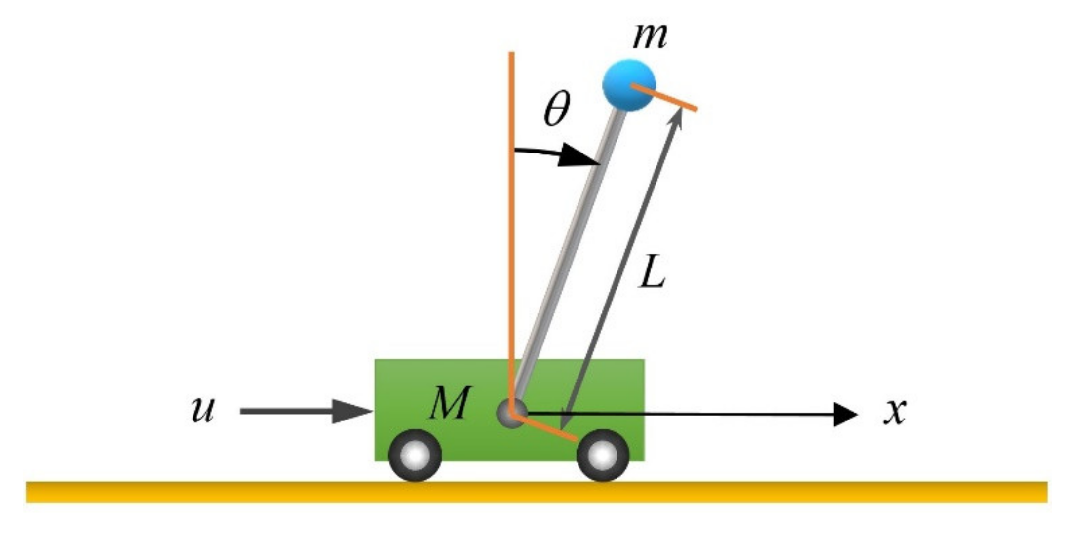
Let us consider an inverted pendulum system (Figure 1).

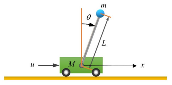
Figure 1. Schematic of an inverted pendulum system.

We assume that the length of the linear cart rail is 2 m and the middle point is $x=0$; the pendulum rod is rigid and massless. All frictional forces in the system can be neglected. Under such an assumption, the entire pendulum mass is concentrated at the center of the pendulum ball. The symbol definitions and simulation conditions for this system are as follows:

• $M=0.5$ kg (cart mass);
• $m=0.1$ kg (ball mass);
• $L=0.3$ m (distance from the pendulum pivot to the center of the ball);
• $g=9.8$ m/s² (gravity constant);
• $\theta$ (rad): rotational displacement of the pendulum;
• $x$ (m): horizontal displacement of the cart; and
• $u$ (N): control force,

where $u$ is subjected to the following saturation condition:

$$u=\left\{\begin{array}{c} 30,\\ u,\\ -30,\end{array} \right.\begin{array}{l}\mathrm{if} u>u_{\max }=30\hfill \\ \mathrm{if} u_{\min }\le u\le u_{\max }\hfill \\ \mathrm{if} u<u_{\min }=-30\hfill \end{array}$$

(10)

The dynamic equation of the inverted pendulum is expressed as follows [34,35]:

$$\ddot{\theta }=\frac{ u\cos \theta -\left(M+m\right)g\sin \theta +mL\left(\cos \theta \sin \theta \right){\dot{\theta }}_2^2}{mL{\cos }^2\theta -\left(M+m\right)L}$$

(11)

$$\ddot{x}=\frac{ u+mL\sin \theta {\dot{\theta }}_2^2-mg\left(\cos \theta \sin \theta \right) }{ M+m-m{\cos }^2\theta }$$

(12)

The state variables of the system are defined as follows:

$$x_1=\theta , x_2=\dot{\theta } , x_3=x, x_4=\dot{x}$$

(13)

The dynamic equation of the inverted pendulum system can be rewritten as follows:

$${\dot{x}}_1=x_2$$

(14)

$${\dot{x}}_2=\frac{ u\cos x_1-\left(M+m\right)g\sin x_1+mL\left(\cos x_1\sin x_1\right)x_2^2}{mL{\cos }^2{x}_1-(M+m)L}$$

(15)

$${\dot{x}}_3=x_4$$

(16)

$${\dot{x}}_4=\frac{ u+mL\left(\sin x_1\right)x_2^2-mg\left(\cos x_1\sin x_1\right) }{ M+m-m{\cos }^2{x}_1}$$

(17)

The state vector is defined as follows:

$$x=\left[\begin{array}{c}{x}_1\\ x_2\\ x_3\\ x_4\end{array}\right]=\left[\begin{array}{c}\theta \\ \dot{\theta }\\ x\\ \dot{x}\end{array}\right]$$

(18)

In this example, we assume that the states $x_1=\theta$ and $x_3=x$ can be measured but are disturbed by $v_{\theta }$ and $v_x$, respectively. Both $v_{\theta }$ and $v_x$ are Gaussian noises with a mean value of zero and a standard deviation of 0.0001. The states $x_2=\dot{\theta }$ and $x_4=\dot{x}$ are estimated using the Euler method, where $\dot{\theta }\cong \left(\theta (k)-\theta (k-1)\right)/\Delta t$ and $\dot{x}\cong \left(x(k)-x(k-1)\right)/\Delta t$. The controller used in the inverted pendulum system is the following state feedback controller:

$$u=-kx\equiv -\left[\begin{array}{cccc}{k}_1& k_2& k_3& k_4\end{array}\right]\left[\begin{array}{c}{x}_1\\ x_2\\ x_3\\ x_4\end{array}\right]=-k_1{x}_1-k_2{x}_2-k_3{x}_3-k_4{x}_4$$

(19)

The purpose of control is to fix the cart at the middle point of the rail and to maintain the angle between the inverted pendulum and the plumb line at 0. In addition, the initial state is $x={\left[\begin{array}{cccc}0.7& 0& 0& 0\end{array}\right]}^T$; the sampling time $\Delta t$ is 0.002 s; the simulation termination time $T_f$ is 2 s; the allowable variation range of the pendulum is $-{\theta }_{\max }={\theta }_{\min }\le \theta \le {\theta }_{\max }$, where ${\theta }_{\max }=0.7$; the allowable range of the cart is $-x_{\max }=x_{\min }\le x\le x_{\max }$, where $x_{\max }=0.8$; and $T_r$ denotes the time at which $\theta$ or $x$ moves out of the allowable range. Additionally, the discrete performance index is defined as follows:

$$J={\displaystyle \sum _{k=1}^{N_f}k\left(\frac{\left|\theta (k)\right|}{{\theta }_{\max }}+\frac{\left|x(k)\right|}{x_{\max }}\right)}+W_r\left(T_f-T_r\right)$$

(20)

where $N_f\equiv T_f/\Delta t=1000$ and $N_r\equiv T_r/\Delta t$. $W_r$ is the weighting of the penalty function. When the output signal remains within the allowable range within the termination time $T_f$, $W_r$ is zero. Conversely, if the output signal leaves the allowable range before the time reaches $T_f$, then $W_r$ is a positive constant that is much higher than the value of the first term on the right-hand side of the equation in function (20). A useful reference value is $W_r\cong N_f^2\left({\theta }_{\max }/{\theta }_{\max }+x_{\max }/x_{\max }\right)=2N_f^2$. The actual value used in this example is ${10}^6$. According to the above description, we define $W_r$ in this example as follows:

$$W_r=\left\{\begin{array}{c}{10}^6,\\ 0,\end{array}\right. \begin{array}{l}\mathrm{if} \theta \mathrm{or} x \mathrm{exceeds} \mathrm{the} \mathrm{allowable} \mathrm{range} \mathrm{at} \mathrm{the} N_r\mathrm{th} \mathrm{sampling}\hfill \\ \mathrm{otherwise}\hfill \end{array}$$

(21)

When the output $\theta$ or $x$ is not within the allowable range, along with adding the penalty function to the performance index, we also immediately terminate (stop) the control.

Because the state feedback controller used in this example has four parameters, we first arbitrarily design five sets of controller parameters as the five vertices of the initial simplex. The five sets of parameters and the corresponding performance indices are listed in Table 2. The time responses of the system are shown in Figure 2. Among these, the parameters $p_0$ and $p_1$ can keep the system state within the allowable safe range before the time reaches $T_f$; therefore, both the penalty function values are 0 and the corresponding index values are small. When using $p_2$, $p_3$, and $p_4$, all corresponding states exceed the allowable range before the time reaches $T_f$. Therefore, the penalty function achieves the expected effect that the corresponding index values are much larger than the index values corresponding to both $p_0$ and $p_1$. From this result, it can also be seen that the earlier the simulation/experiment is interrupted, the larger the corresponding index value (representing a worse corresponding parameter).

Table 2. Initial controller parameters for the inverted pendulum system.

$i$	$p_i=\left[\begin{array}{cccc}{k}_1& k_2& k_3& k_4\end{array}\right]$	$J_i=J\left(p_i\right)$
0	$p_0=\left[\begin{array}{cccc}-200& -10& -80& -10\end{array}\right]$	$J_0=1.941\times {10}^5$
1	$p_1=\left[\begin{array}{cccc}-150& -100& -150& -100\end{array}\right]$	$J_1=4.293\times {10}^5$
2	$p_2=\left[\begin{array}{cccc}-100& -20& -150& -20\end{array}\right]$	$J_2=5.651\times {10}^8$
3	$p_3=\left[\begin{array}{cccc}-80& -150& -100& -30\end{array}\right]$	$J_3=7.300\times {10}^8$
4	$p_4=\left[\begin{array}{cccc}-5& -5& -5& -5\end{array}\right]$	$J_4=7.560\times {10}^8$

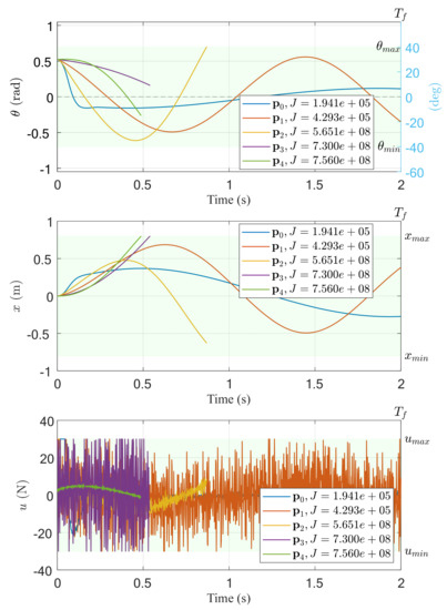
Figure 2. Time responses of the inverted pendulum system controlled by the five sets of controller parameters given in Table 2.

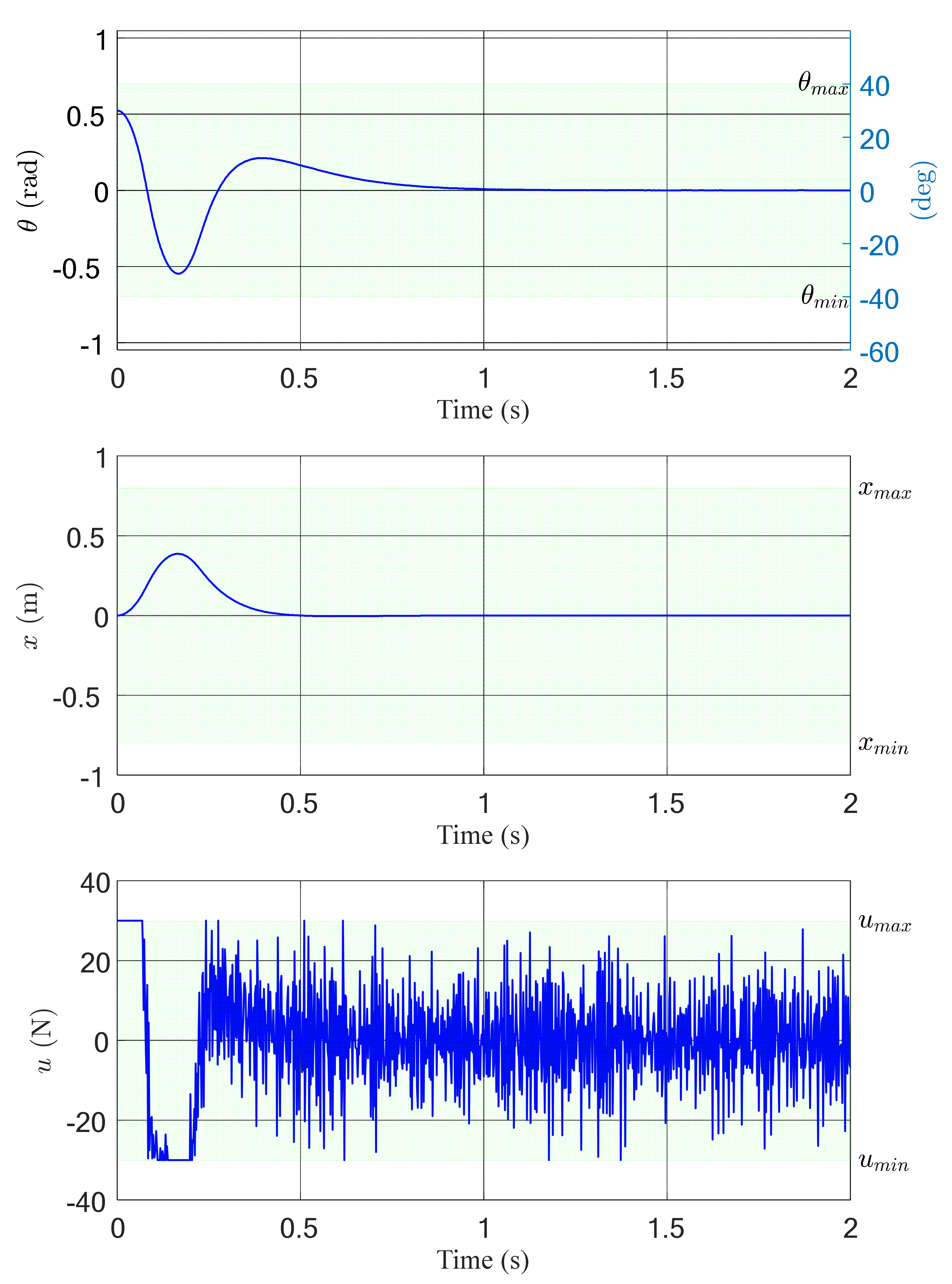
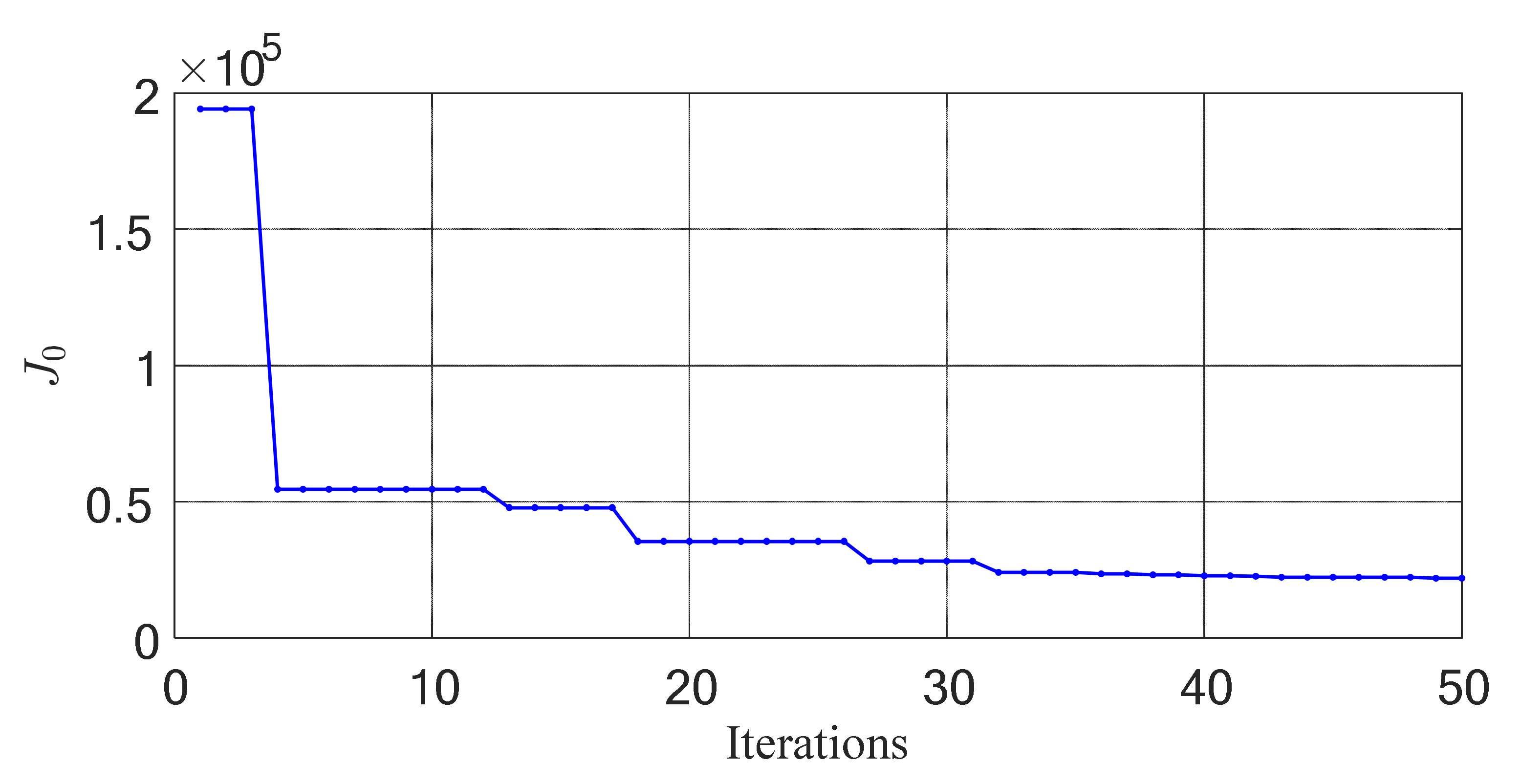
Then, we used the above five sets of parameters as the five vertices of the initial simplex. We set the maximum number of iterations for searching the optimal parameters to 50. The results obtained using the N–M simplex optimal search method are shown in Figure 3 and Figure 4, where the resulting parameters are $k_1=-276.7$, $k_2=-48.12$, $k_3=-289.5$, and $k_4=-122.1$. The corresponding performance index is $J=2.292\times {10}^4$, which is also lower than those for the initial four sets of controllers.

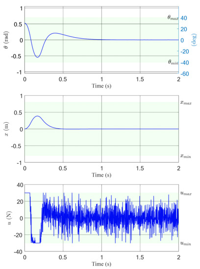
Figure 3. Time response of the inverted pendulum system controlled by the state feedback controller in which the parameters are searched via the N–M simplex method based on the initial vertices given in Table 2.

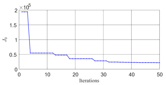
Figure 4. Convergence graph of performance index $J_0$ when the simplex method based on the initial vertices given in Table 2 is used to search for the controller parameters of the inverted pendulum system.

Obtaining a global optimal controller for nonlinear systems is difficult, especially when the dynamic equation of the system is unknown and the state or output signal includes measurement noise. Therefore, the results obtained in the above examples may be local optimal controllers based on specific initial conditions. In practical applications, the most important goal is to design a stable or robust controller effectively, not necessarily to obtain a global optimal controller.

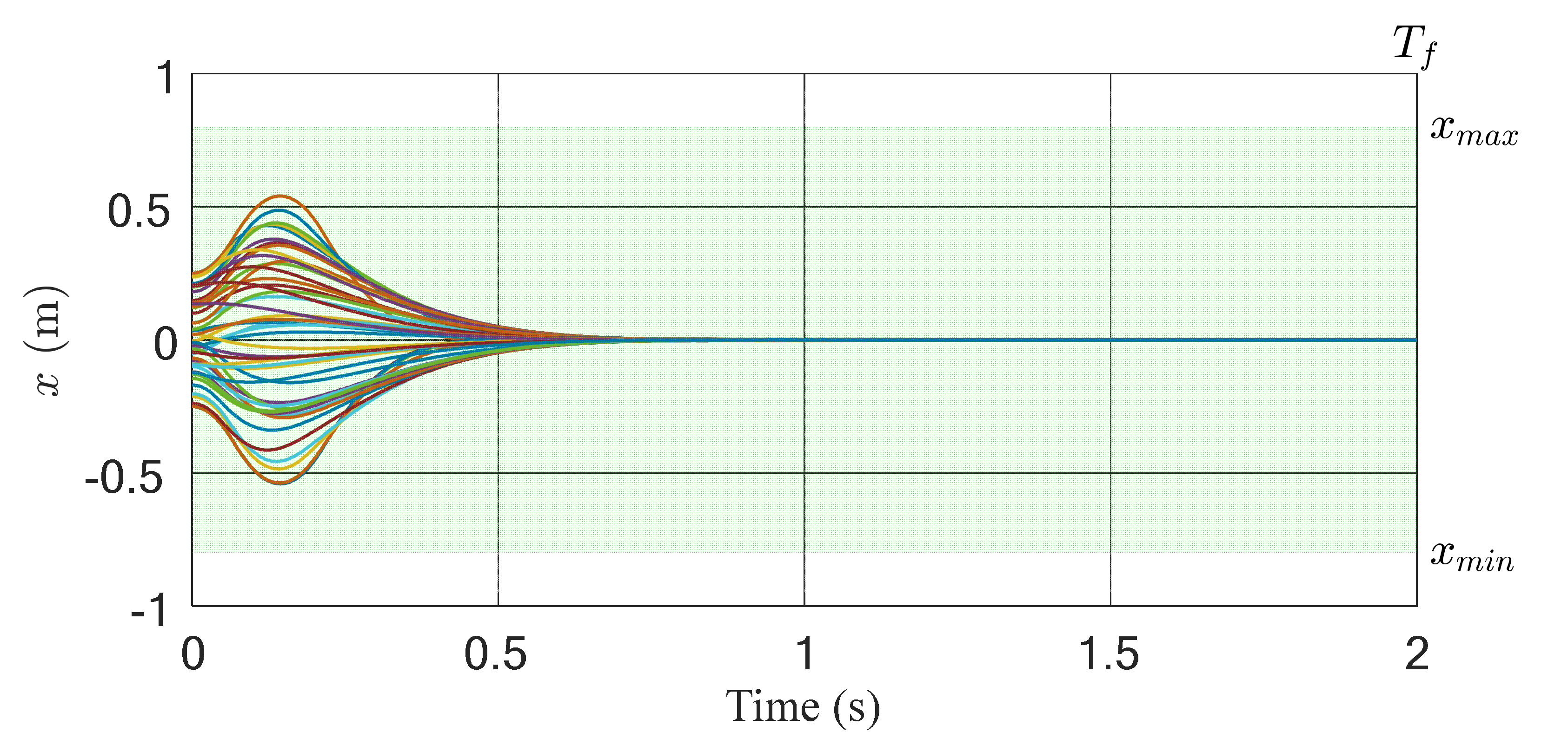
To demonstrate the feasibility of this method, we simulated the above inverted pendulum system with the same state feedback controller, $u=kx$$=\left[\begin{array}{cccc}-276.7& -48.12& -289.5& -122.1\end{array}\right]x$. In this simulation, we used 50 different states as initial conditions. The distribution ranges of the initial states were $x_1(0)=\theta (0)\in [-0.349, 0.349 ]$ (or $[-{20}^{\circ }{, 20}^{\circ } ]$), $x_2(0)=\dot{\theta }(0)=0$, $x_3(0)=x(0)\in [-0.25, 0.25 ]$, and $x_4(0)=\dot{x}(0)=0$. Figure 5 shows the time responses of the above simulation. The results show that the 50 different initial states approached equilibrium within 2 s.

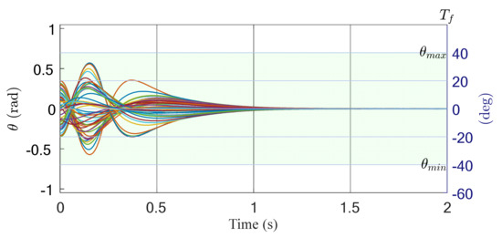
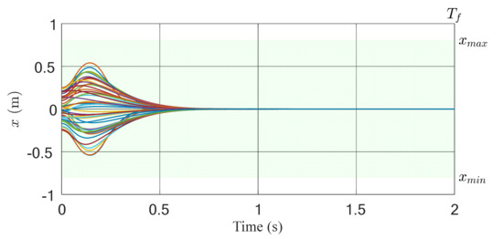
Figure 5. Time response of the inverted pendulum system controlled by the state feedback controller $u=kx$$=\left[\begin{array}{cccc}-276.7& -48.12& -289.5& -122.1\end{array}\right]x$ with 50 different random initial states.

4. Conclusions

In this study, we proposed a systematic method for designing optimal controllers for systems with unknown dynamic equations. First, we proposed an original performance index based on the characteristics and control aim of the controlled system. The performance index can include the state, output, error, or control input of the system. To ensure that this performance index was applicable even when the state or output of the system was not within the allowable safety range, we added a key penalty function. Then, we used the N–M simplex method to search for the optimal controller parameters iteratively. In addition to the ease of implementation of the N–M simplex method, another important advantage of the algorithm is that it only needs all the signals in the performance index to be available, without the need to know the dynamic equation of the system in advance.

To demonstrate the feasibility of the proposed method, we adopted an inverted pendulum system with measurement noise as the example. The simulation results showed that even if the initial controller parameters could not stabilize the system, after the algorithm reached the iterative termination condition, not only was the system stable but it also exhibited good transient response performance.

The optimal controller parameter search method proposed in this study has the following advantages: (1) the dynamic equation of the system need not be known; (2) the method can be used regardless of the stability of the open-loop system; (3) the method can be applied to both linear and nonlinear systems; (4) the method can be used in systems containing measurement noise; and (5) the systematic nature of the method can improve the design efficiency.

References

- Slotine, J.-J.E.; Li, W. Applied Nonlinear Control; Prentice Hall: Englewood Cliffs, NJ, USA, 1991. [Google Scholar]
- Khalil, H. Nonlinear Systems, 3rd ed.; Prentice Hall: Upper Saddle River, NJ, USA, 2002. [Google Scholar]
- Tavasoli, A.; Enjilela, V. Active disturbance rejection and Lyapunov redesign approaches for robust boundary control of plate vibration. Int. J. Syst. Sci. 2017, 48, 1656–1670. [Google Scholar] [CrossRef]
- Xu, J.; Fridman, L.M.; Fridman, E.; Niu, Y. Output-feedback Lyapunov redesign of uncertain systems with delayed measurements. Int. J. Robust Nonlinear Control 2021, 31, 3747–3766. [Google Scholar] [CrossRef]
- Zhou, L.; Zhang, J.; She, H.; Jin, H. Quadrotor UAV flight control via a novel saturation integral backstepping controller. Automatika 2019, 60, 193–206. [Google Scholar] [CrossRef]
- Fang, Y.; Fei, J.; Yang, Y. Adaptive backstepping design of a microgyroscope. Micromachines 2018, 9, 338. [Google Scholar] [CrossRef] [Green Version]
- Mossa, M.A.; Echeikh, H. A novel fault tolerant control approach based on backstepping controller for a five phase induction motor drive: Experimental investigation. ISA Trans. 2021, 112, 373–385. [Google Scholar] [CrossRef]
- Liu, Z.; Han, Z.; Zhao, Z.; He, W. Modeling and adaptive control for a spatial flexible spacecraft with unknown actuator failures. Sci. China Inf. Sci. 2021, 64, 152208. [Google Scholar] [CrossRef]
- Liang, H.; Liu, G.; Zhang, H.; Huang, T. Neural-network-based event-triggered adaptive control of nonaffine nonlinear multiagent systems with dynamic uncertainties. IEEE Trans. Neural Netw. Learn. Syst. 2021, 32, 2239–2250. [Google Scholar] [CrossRef]
- Wang, S.; Na, J. Parameter estimation and adaptive control for servo mechanisms with friction compensation. IEEE Trans. Ind. Inform. 2020, 16, 6816–6825. [Google Scholar] [CrossRef]
- Utkin, V.I. Variable structure systems with sliding modes. IEEE Trans. Autom. Control 1977, 22, 212–222. [Google Scholar] [CrossRef]
- Šabanovic, A. Variable structure systems with sliding modes in motion control—A survey. IEEE Trans. Ind. Inform. 2011, 7, 212–223. [Google Scholar] [CrossRef]
- Wang, J.; Zhu, P.; He, B.; Deng, G.; Zhang, C.; Huang, X. An adaptive neural sliding mode control with eso for uncertain nonlinear systems. Int. J. Control Autom. Syst. 2021, 19, 687–697. [Google Scholar] [CrossRef]
- Shao, K.; Zheng, J.; Wang, H.; Xu, F.; Wang, X.; Liang, B. Recursive sliding mode control with adaptive disturbance observer for a linear motor positioner. Mech. Syst. Signal Process. 2021, 146, 107014. [Google Scholar] [CrossRef]
- Charfeddine, S.; Jerbi, H. A survey on non-linear gain scheduling design control for continuous and discrete time systems. Int. J. Model. Identif. Control 2013, 19, 203–216. [Google Scholar] [CrossRef]
- Liu, C.; Zhao, W.; Li, J. Gain scheduling output feedback control for vehicle path tracking considering input saturation. Energies 2020, 13, 4570. [Google Scholar] [CrossRef]
- Accetta, A.; Alonge, F.; Cirrincione, M.; D’Ippolito, F.; Pucci, M.; Rabbeni, R.; Sferlazza, A. Robust control for high performance induction motor drives based on partial state-feedback linearization. IEEE Trans. Ind. Appl. 2019, 55, 490–503. [Google Scholar] [CrossRef]
- Wu, J.; Lu, Y. Exact feedback linearisation optimal control for single-inductor dual-output boost converter. IET Power Electron. 2020, 13, 2293–2301. [Google Scholar] [CrossRef]
- Owczarkowski, A.; Horla, D.; Zietkiewicz, J. Introduction of feedback linearization to robust LQR and LQI control– analysis of results from an unmanned bicycle robot with reaction wheel. Asian J. Control. 2018, 21, 1028–1040. [Google Scholar] [CrossRef]
- Spendly, W.; Hext, G.R.; Himsworth, F.R. Sequential application of simplex designs in optimisation and evolutionary operation. Technometrics 1962, 4, 441–461. [Google Scholar] [CrossRef]
- Nelder, J.A.; Mead, R. A simplex method for function minimization. Comput. J. 1965, 7, 308–313. [Google Scholar] [CrossRef]
- Lagarias, J.C.; Reeds, J.A.; Wright, M.H.; Wright, P.E. Convergence properties of the Nelder-Mead simplex method in low dimensions. SIAM J. Optim. 1998, 9, 112–147. [Google Scholar] [CrossRef] [Green Version]
- McKinnon, K.I.M. Convergence of the Nelder-Mead simplex method to a nonstationary point. SIAM J. Optim. 1998, 9, 148–158. [Google Scholar] [CrossRef]
- Byatt, D. Convergent Variants of the Nelder-Mead Algorithm. Master’s Thesis, University of Canterbury, Christchurch, New Zealand, 2000. [Google Scholar] [CrossRef]
- Price, C.J.; Coope, I.D.; Byatt, D. A convergent variant of the Nelder-Mead algorithm. J. Optim. Theory Appl. 2002, 113, 5–19. [Google Scholar] [CrossRef] [Green Version]
- Fuh, C.-C.; Tsai, H.-H.; Lin, H.-C. Parameter identification of linear time-invariant systems with large measurement noises. In Proceedings of the 2016 12th World Congress on Intelligent Control and Automation (WCICA), Guilin, China, 12–15 June 2016; pp. 2874–2878. [Google Scholar] [CrossRef]
- Xu, S.; Wang, Y.; Wang, Z. Parameter estimation of proton exchange membrane fuel cells using eagle strategy based on JAYA algorithm and Nelder-Mead simplex method. Energy 2019, 173, 457–467. [Google Scholar] [CrossRef]
- Lee, Y.; Resiga, A.; Yi, S.; Wern, C. The optimization of machining parameters for milling operations by using the Nelder–Mead simplex method. J. Manuf. Mater. Process. 2020, 4, 66. [Google Scholar] [CrossRef]
- Niegodajew, P.; Marek, M.; Elsner, W.; Kowalczyk, Ł. Power plant optimisation—Effective use of the Nelder-Mead approach. Processes 2020, 8, 357. [Google Scholar] [CrossRef] [Green Version]
- Zettel, V.; Hitzmann, B. Optimization of the production parameters for bread rolls with the Nelder–Mead simplex method. Food Bioprod. Process. 2017, 103, 10–17. [Google Scholar] [CrossRef]
- Naidu, D.S. Optimal Control. Systems; CRC Press: Boca Raton, FL, USA, 2003. [Google Scholar]
- Anderson, B.D.O.; Moore, J.B. Optimal Control: Linear Quadratic Methods; Prentice-Hall: Englewood Cliffs, NJ, USA, 1990. [Google Scholar]
- Dorf, R.C.; Bishop, R.H. Modern Control. Systems, 12th ed.; Prentice Hall: Englewood Cliffs, NJ, USA, 2014. [Google Scholar]
- Mahmoodabadi, M.J.; Haghbayan, H.K. An optimal adaptive hybrid controller for a fourth-order under-actuated nonlinear inverted pendulum system. Trans. Inst. Meas. Control 2019, 42, 285–294. [Google Scholar] [CrossRef]
- Waszak, M.; Langowski, R. An automatic self-tuning control system design for an inverted pendulum. IEEE Access 2020, 8, 26726–26738. [Google Scholar] [CrossRef]
Publisher’s Note: MDPI stays neutral with regard to jurisdictional claims in published maps and institutional affiliations. |
© 2021 by the authors. Licensee MDPI, Basel, Switzerland. This article is an open access article distributed under the terms and conditions of the Creative Commons Attribution (CC BY) license (https://creativecommons.org/licenses/by/4.0/).