Abstract
The most popular method for computing the matrix logarithm is a combination of the inverse scaling and squaring method in conjunction with a Padé approximation, sometimes accompanied by the Schur decomposition. In this work, we present a Taylor series algorithm, based on the free-transformation approach of the inverse scaling and squaring technique, that uses recent matrix polynomial formulas for evaluating the Taylor approximation of the matrix logarithm more efficiently than the Paterson–Stockmeyer method. Two MATLAB implementations of this algorithm, related to relative forward or backward error analysis, were developed and compared with different state-of-the art MATLAB functions. Numerical tests showed that the new implementations are generally more accurate than the previously available codes, with an intermediate execution time among all the codes in comparison.
1. Introduction and Notation
The calculus of matrix functions has been, for a long period of time, an area of interest in applied mathematics due to its multiple applications in many branches of science and engineering; see [1] and the references therein. Among these matrix functions, the matrix exponential stands out due to both its applications and the difficulties of its effective calculation. Basically, given a square matrix , its exponential function is defined by the matrix series:
Directly related to the exponential function, we find the matrix logarithm. Specifically, given a nonsingular matrix whose eigenvalues lie in , we define the matrix logarithm of A as any matrix satisfying the matrix equation:
Of course, there are infinite solutions of Equation (1), but we only focus on the principal matrix logarithm or the standard branch of the logarithm, denoted by , which is the unique logarithm of matrix A (see Theorem 1.31 of [1]) whose eigenvalues all lie in the strip . Indeed, this principal matrix logarithm is the most used in applications in many fields of research from pure science to engineering [2], such as quantum chemistry and mechanics [3,4], buckling simulation [5], biomolecular dynamics [6], machine learning [7,8,9,10], graph theory [11,12], the study of Markov chains [13], sociology [14], optics [15], mechanics [16], computer graphics [17], control theory [18], computer-aided design (CAD) [19], optimization [20], the study of viscoelastic fluids [21,22], the analysis of the topological distances between networks [23], the study of brain–machine interfaces [24], and also in statistics and data analysis [25], among other areas. Just considering various branches of engineering, the matrix logarithm can be employed to compute the time-invariant component of the state transition matrix of ordinary differential equations with periodic time-varying coefficients [26] or to recover the coefficient matrix of a differential system governed by the linear differential equation from observations from the state vector y [27].
The applicability of the matrix logarithm in so many distinct areas has motivated different approaches for its evaluation. One of the most-used methods was that proposed by Kenney and Laub in [28], based on the inverse scaling and squaring method and a Padé approximation, exploiting the matrix identity:
This method finds an integer s such that is close to the identity matrix, approximates by a [p/q] Padé approximation , and finally, computes .
These same authors developed in [27] an algorithm that consists of obtaining the Schur decomposition , where Q is a unitary matrix, T is an upper triangular matrix, and is the conjugate transpose of Q. Then, is computed as follows: the main diagonal is calculated by applying the logarithm scalar function on its elements, and the upper diagonals are computed by using the Fréchet derivative of the logarithm function. Finally, is computed as .
Later, most of the developed algorithms basically used the inverse scaling and squaring method with Padé approximants to dense or triangular matrices; see [29,30,31,32,33,34,35]. Nevertheless, some new algorithms are based on other methods, among which the following can be highlighted:
- An algorithm based on the arithmetic–geometric mean iteration; see [36];
- The use of contour integrals; see [37];
- Methods based on different quadrature formulas, proposed in [38,39].
Finally, we should mention the built-in MATLAB function, called logm, that computes the principal matrix logarithm by means of the algorithms described in [32,33].
Throughout this paper, we refer to the identity matrix of order n as , or I. In addition, we denote by the set of eigenvalues of a matrix , whose spectral radius is defined as:
With , we denote the result reached after rounding x to the nearest integer greater than or equal to x, and is the result reached after rounding x to the nearest integer less than or equal to x. The matrix norm stands for any subordinate matrix norm; in particular, is the usual 1-norm. Recall that if is a matrix in , its 2-norm or Euclidean norm represented by satisfies [40]:
All the implemented codes in this paper are intended for IEEE double-precision arithmetic, where the unit round off is . Their implementations for other distinct precisions are straightforward.
This paper is organized as follows: Section 2 describes an inverse scaling and squaring Taylor algorithm based on efficient evaluation formulas [41] to approximate the matrix logarithm, including an error analysis. Section 3 includes the results corresponding to the experiments performed in order to compare the numerical and computational performance of different codes against a test battery composed of distinct types of matrices. Finally, Section 4 presents the conclusions.
2. Taylor Approximation-Based Algorithm
If , then (see [1], p. 273):
Taylor approximation is given by:
where all the coefficients are positive and m denotes the order of the approximation.
For the lower orders , 2, and 4, the corresponding polynomial approximations from (3) use the Paterson–Stockmeyer method for the evaluation. For the Taylor approximation orders , Sastre evaluation formulas from [41,42] are used for evaluating Taylor-based polynomial approximations from (3) more efficiently than the Paterson–Stockmeyer method. For reasons that will be shown below, the Taylor approximation of , denoted by , is used in all the Sastre approximations and evaluation formulas of the matrix logarithm.
Sastre approximations and evaluation formulas based on (4) are denoted as , where the superscript stands for the type of polynomial approximation used, in this case the Taylor polynomial (4), and the subindex m represents the maximum degree of the polynomial for the corresponding polynomial approximation. Using (3) and (4), the implementation for the matrix logarithm computation is based on:
For , we see that . However, for higher orders of approximation, we show that has some more terms than . These terms are similar to, but different from the respective ones of the Taylor series. Following [43] (Section 4), we represent this order of approach by , and its corresponding approximation is denoted by . The next subsections deal with the different evaluation formulas and approximations.
2.1. Evaluation of
For , the following evaluation formulas from [41] (Example 3.1) are used:
where the second subindex in and expresses the maximum power of the matrix A that appears in each expression, i.e., . The sum of both subindices in and gives the cost in terms of matrix products for evaluating each formula, denoted from now on by C. Thus, for and for .
The system of nonlinear equations to be solved in order to determine the coefficients in (6) that arise when equating , where is a general matrix polynomial:
is given by (16)–(24) of [41], i.e.,
From (7), one obtains . Since in (3), we equate from (4), where the corresponding coefficient is positive to prevent from being a complex number.
This system can be solved analytically using (25)–(32) from [41] (Example 3.1), giving four sets of exact solutions for the coefficients in (6). Then, the solutions are rounded to the desired precision arithmetic. As mentioned before, we use IEEE double-precision arithmetic. From now on, for any coefficient , denotes the corresponding one rounded to that precision.
In order to check if the rounded coefficient solutions are sufficiently accurate to evaluate (6), we follow the stability check of [41] (Example 3.1). It consists of substituting the rounded coefficients into the original system of Equations (7)–(15) and testing if the relative error given by them with respect to each coefficient , for , is lower than the unit round off in IEEE double-precision arithmetic. For instance, from (12), it follows that the relative error for is:
Then, we select a set of solutions where the relative errors for all , for , are lower than u. In our experience, solutions giving relative errors of order also provide accurate results. Finally, the approximation is computed as:
where is evaluated using (6) with the coefficients from Table 1.

Table 1.
Coefficients for computing the matrix logarithm Taylor approximation of order , using Sastre evaluation Formula (6), as .
2.2. Evaluation of Higher-Order Taylor-Based Approximations
For higher orders of approximation, we followed a similar procedure as that described in [43] (Sections 3.2 and 3.3), where evaluation formulas for Taylor-based approximations of the matrix exponential of orders and were given. Both of these formulas were generalized to any polynomial approximation in [42] (Section 3), and this type of polynomial approximation evaluation formula was first presented in [41] (Example 5.1). Following the notation given in [43] (Section 4), the suffix “+” in m means that the corresponding Taylor-based approximation is more accurate than the Taylor one of order m. This is because the approximation with the order denoted by has some more polynomial terms than the Taylor one of order m, and these terms are similar to the corresponding Taylor approach terms. We numerically define this similarity in each case.
Proposition 1 and the MATLAB code fragments from [42] (Section 3.1) allow obtaining all the solutions for the coefficients of the evaluation formulas (10)–(12) from [43] (Section 3.2), not only for the exponential Taylor approximation of order , but for whatever polynomial approximation of the same order. Unfortunately, there were no real solutions for the evaluation formulas of the logarithm Taylor approximation of order . We also tested different variations of the formulas providing order ; however, there were no real solutions for any of them. The same also occurred in [44] (Section 2.2) with the hyperbolic tangent Taylor approximation of order . In that case, we could find real solutions using an approximation of order . In this case, there were also real solutions for the following logarithm Taylor approximation evaluation formulas of order :
where it is easy to show that the degree of is 16. Therefore, we denote this approximation by , and similarly to [44] (Section 2.2), one obtains:
where is given by (4) and and depend on the coefficients from (18). From (4), one obtains that and . From all the solutions obtained for the coefficients, a stable one was selected that incurs in relative errors lower than one with respect to the corresponding Taylor coefficients and , concretely:
showing two decimal digits.
For orders from to , we first evaluate and store the matrix powers for , and then, the evaluation formulas (94)–(96) proposed in [42] (p. 21) are used, reproduced here for the sake of clarity:
The degree of is , and the total number of coefficients of is , i.e., coefficients , s coefficients , s coefficients , coefficients , and coefficients , , and ; see [42] (p. 21). Analogous to (6), the cost C for evaluating , , from (21), (23) and (24) in terms of the matrix products is .
Again, the corresponding approximation from (24), denoted as , allows us to evaluate Taylor-based approximations of the matrix logarithm of the type:
where the coefficients depend on the ones from (21)–(24).
In order to obtain all coefficients from these expressions, the nested procedure used in [43] (Sections 3.2 and 3.3) was applied. Analogous to [44] (p. 7), we employed the vpasolve function from the MATLAB Symbolic Computation Toolbox (https://es.mathworks.com/help/symbolic/vpasolve.html, accessed on 20 August 2021) with the random option to obtain different solutions of the nonlinear system arising for each order of approximation. Concretely, we obtained 1000 solutions for the coefficient sets of (21), (22), and (24) for orders and and 300 solutions for . Then, the most stable real solution according to the stability check from [41] (Example 3.1) (see (16)) was selected for each order .
Similar to (20), we checked that the relative error for coefficients , , from (27) with respect to the corresponding Taylor coefficients for the selected solutions was less than one.
For the orders higher than , we combined from (24) with the Paterson–Stockmeyer method, similar to (52) from [41] (Proposition 1), giving:
where p is a multiple of s and the resulting Taylor-based approximation order is . If , note that . Therefore, the corresponding approximation (26) is denoted by , and it allows us to evaluate Taylor-based approximations of the matrix logarithm of the type:
Table 2 shows the orders of approximations available using the Paterson–Stockmeyer method or and their differences for a given cost C in terms of matrix products. It also shows the corresponding values of s and p for (26). Table 2 shows that the difference in the polynomial orders increases as C grows. See the function available at http://personales.upv.es/~jorsasma/Software/logm_pol.m for implementation details (accessed on 20 August 2021).
Table 2.
Maximum available approximation order for a cost C in terms of matrix products using the Paterson–Stockmeyer method, denoted by , the maximum order using from (27), denoted by , and the difference . Parameters s and p are used in in each case.
2.3. Error Analysis
On the one hand, the relative forward error of approximating by means of can be defined as:
where is any of the Sastre approximations that appear in Section 2.1 and Section 2.2. This error can be expressed as:
Using Theorem 1.1 from [45], one obtains:
where:
Let be:
On the other hand, the absolute backward error can be defined as the matrix that verifies:
Then:
whereby the backward error can be expressed as:
It can be proven that this error can be expressed as ; hence, the relative backward error of approximating by means of can be bounded as follows:
where
Let be:
The values of and , listed in Table 3, were obtained by using symbolic computations. They satisfy that and , for . Hence, the numerical performance of two different algorithms, each based on one of these error formulations, will be very similar. Taking into account (28) and (30)–(32), if , then:
and:
i.e., the relative forward and backward errors are lower than the unit round off in IEEE double-precision arithmetic.
Table 3.
Values and , , corresponding to the forward and backward error analyses, respectively.
However, if only , then:
i.e., only the relative backward error is lower than the unit round off.
2.4. Algorithm for Computing
Taking into account that can be expressed as , Algorithm 1 computes by the inverse scaling and squaring Taylor algorithm based on the expressions that appear in Section 2.1 and Section 2.2, where , , is a Taylor approximation order. In this algorithm, we can use either the (forward error analysis) or the (backward error analysis) of Table 3.
The preprocessing step is based on applying a similarity transformation of matrix A to obtain a permutation of a diagonal matrix T whose elements are integer powers of two and a new balanced matrix B such that . The aim of balancing is to achieve the norms of each row of B and its corresponding column nearly equal, trying to concentrate any ill-conditioning of the eigenvalues of matrix A into the diagonal scaling matrix T. To carry out this balancing, the balance MATLAB function can be employed.
Steps 2 to 11 bring A close to I by taking successive square roots of A until , where is the maximum order and is computed as described in Step 5. To compute the matrix square roots required, we implemented a MATLAB function that uses the scaled Denman–Beavers iteration described in [1] (Equation (6.28)). This iteration is defined by:
with , , and , n being the dimension of matrix A. Although convergence is not guaranteed, if it does, then converges to . In Step 5, we use the following approximation for calculating from (29) (see [46,47]):
To compute approximately the 1-norm of and , the 1-norm estimation algorithm of [48] can be employed. In order to implement Algorithm 1 in the most efficient way, it is worth noting that should be only worked out if .
| Algorithm 1 Given a matrix , a maximum approximation order , , and a maximum number of iterations , this algorithm computes by a Taylor approximation of order lower that or equal to . |
|
Then, Step 12 finds the most appropriate order of the approximation polynomial to be used, always with the aim of reducing the computational cost, but without any loss of accuracy. For efficiency reasons, an algorithm based on the well-known bisection method of function root search was adopted. In Step 13, the matrix logarithm approximation of is computed by means of the efficient polynomial evaluations presented in Section 2.1 and Section 2.2. Finally, the squaring phase takes place in Step 14, and in Step 15, the postprocessing operation is required to provide the logarithm of matrix A if the preprocessing stage was previously applied to it.
3. Numerical Experiments
In this section, we compare the following five MATLAB codes in terms of accuracy and efficiency:
- logm_iss_full: It calculates the matrix logarithm using the transformation-free form of the inverse scaling and squaring method with Padé approximation. Matrix square roots are computed by the product form of the Denman–Beavers iteration ([1], Equation (6.29)). It corresponds to Algorithm 5.2 described in [32], denoted as the iss_new code;
- logm_new: It starts with the transformation of the input matrix A to the Schur triangular form . Thereafter, it computes the logarithm of the triangular matrix T using the inverse scaling and squaring method with Padé approximation. The square roots of the upper triangular matrix T are computed by the Björck and Hammarling algorithm ([1,49], Equation (6.3)), solving one column at a time. It is an implementation of Algorithm 4.1 explained in [32], designated as the iss_schur_new function;
- logm: It is a MATLAB built-in function in charge of working out the matrix logarithm from the algorithms included in [32,33]. MATLAB R2015b incorporated an improved version that applies inverse scaling and squaring and Padé approximants to the whole triangular Schur factor, whereas the previous logm applied this technique to the individual diagonal blocks in conjunction with the Parlett recurrence. Although it follows a similar main scheme to the logm_new code, the square roots of the upper triangular matrix T are computed using a recursive blocking technique from the Björck and Hammarling recurrence, which works outs the square roots of increasingly smaller triangular matrices [50]. The technique is rich on matrix multiplications and has the requirement of solving the Sylvester equation. In addition, it allows parallel architectures to be exploited simply by using threaded BLAS;
- logm_polf: This is an implementation of Algorithm 1, where Taylor matrix polynomials are evaluated thanks to the Sastre formulas previously detailed. Values from the set were used as the approximation polynomial order for all the tests carried out in this section, and forward relative errors were considered;
- logm_polb: It is an identical implementation to the previous code, but it is based on relative backward errors.
A testbed consisting of the following three sets of different matrices was employed in all the numerical experiments performed. In addition, MATLAB Symbolic Math Toolbox with 256 digits of precision was the tool chosen to obtain the “exact”matrix logarithm, using the vpa (variable-precision floating-point arithmetic) function:
- Set 1: The 100 diagonalizable complex matrices. They have the form , where D is a diagonal matrix with complex eigenvalues and V is an orthogonal matrix such as , H being a Hadamard matrix and n the matrix order. The 2-norm of these matrices varies from to 300. The “exact”matrix logarithm was calculated as ;
- Set 2: The 100 nondiagonalizable complex matrices computed as , where J is a Jordan matrix with complex eigenvalues whose algebraic multiplicity is randomly generated between 1 and 3. V is an orthogonal random matrix with elements in progressively wider intervals from , for the first matrix, to , for the last one. As the 2-norm, these matrices range from to . The “exact”matrix logarithm was computed as ;
- Set 3: The 52 matrices A from the Matrix Computation Toolbox (MCT) [51] and the 20 from the Eigtool MATLAB Package (EMP) [52], all of them with a order. The “exact”matrix logarithm was calculated by means of the following three-step procedure:
- Calling the MATLAB function eig and providing, as a result, a matrix V and a diagonal matrix D such that , using the vpa function. If any of the elements of matrix D, i.e., the eigenvalues of matrix A, have a real value less than or equal to zero, this will be replaced by the result of the sum of its absolute value and a random number in the interval . Thus, a new matrix will be generated. Next, matrices and will be calculated in the form and ;
- Computing the matrix logarithm thanks to the logm and vpa functions, that is ;
- Considering the “exact”matrix logarithm of only if:
A total of forty-six matrices, forty from the MCT and six from the EMP, were considered for the numerical experiments. The others were excluded for the following reasons:- -
- Matrices 17, 18, and 40 from the MCT and Matrices 7, 9, and 14 from the EMP did not pass the previous procedure for the “exact”matrix logarithm computation;
- -
- The relative error incurred by some of the codes in comparison was greater than or equal to unity for Matrices 4, 6, 12, 26, 35, and 38 belonging to the MCT and Matrices 1, 4, 10, 19, and 20 pertaining to the EMP. The reason was the ill-conditioning of these matrices for the matrix logarithm function;
- -
- Matrices 2, 9, and 16, which are part of the MCT, and Matrices 15 and 18, incorporated in the EMP, resulted in a failure to execute the logm_iss_full code. More specifically, the error was due to the fact that the function sqrtm_dbp, responsible for computing the principal square root of a matrix using the product form of the Denman–Beavers iteration, did not converge after a maximum allowed number of 25 iterations;
- -
- Matrices 8, 11, 13, and 16 from the EMP were already incorporated in the MCT.
If we had not taken the previously described precaution of modifying all those matrices with eigenvalues less than or equal to zero, they would have been directly discarded, and evidently, the number of matrices that would be part of this set would be much more reduced.
The accuracy of the distinct codes for each matrix A was tested by computing the normwise relative error as:
where means the “exact”solution and denotes the approximate one. All the tests were carried out on a Microsoft Windows 10 ×64 PC system with an Intel Core i7-6700HQ CPU @2.60Ghz processor and 16 GB of RAM, using MATLAB R2020b.
First of all, three experiments were performed, one for each of the three above sets of matrices, respectively, in order to evaluate the influence of the type of error employed by comparing the numerical and computational performance of logm_polf and logm_polb. Table 4 shows the percentage of cases in which the normwise relative error of logm_polf was lower, greater than, or equal to that of logm_polb. As expected, according to the and values exposed in Table 3, both codes gave almost identical results, with a practically inappreciable improvement for logm_polf in the case of Sets 1 and 3.
Table 4.
Relative error comparison, for the three sets of matrices, between logm_polf and logm_polb.
The computational cost of logm_polf and logm_polb was basically identical, although slightly lower in the case of the latter code, since the logm_polb function required, on some cases, approximation polynomials of lower orders than those of logm_polf. Both of them performed an identical number of matrix square roots.
After analyzing these results, we can conclude that there are no significant differences between the two codes, and either of them could be used in the remainder of this section to establish a comparison with the other ones. Be that as it may, the code chosen to be used for this purpose was logm_polf, and from here on, we designate it as logm_pol, a decision justified by its numerical and computational equivalence to logm_polb.
Having decided which code based on the Taylor approximation to use, we now assess its numerical peculiarities and those of the other methods for our test battery. Table 5 sets out a comparison, in percentage terms, of the relative errors incurred by logm_pol with respect to logm_iss_full, logm_new, and logm.
Table 5.
Relative error comparison, for the three sets of matrices, of logm_pol versus logm_iss_full, logm_new, and logm.
As we can see, logm_pol outperformed logm_iss_full in accuracy in 100% of the matrices in Sets 1 and 2 and 97.83% of them in Set 3. logm_pol achieved better accuracy than logm_new and logm in 97%, 89%, and 89.13% of the matrices for Sets 1, 2, and 3, respectively.
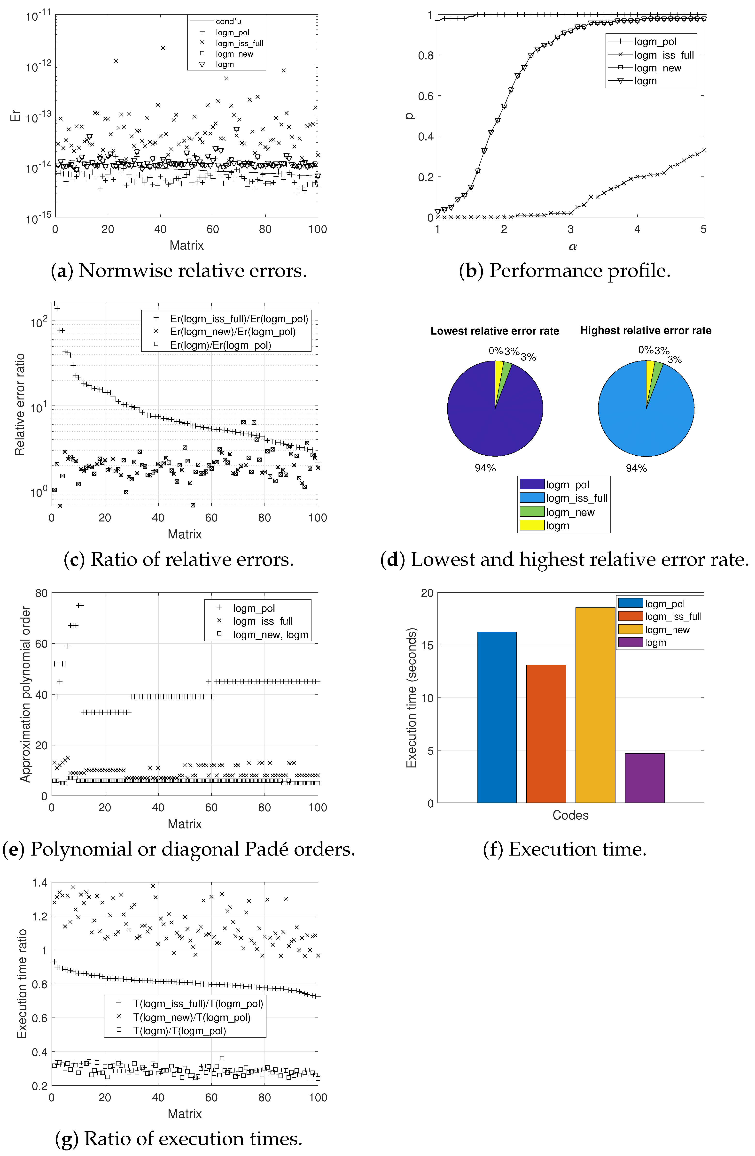
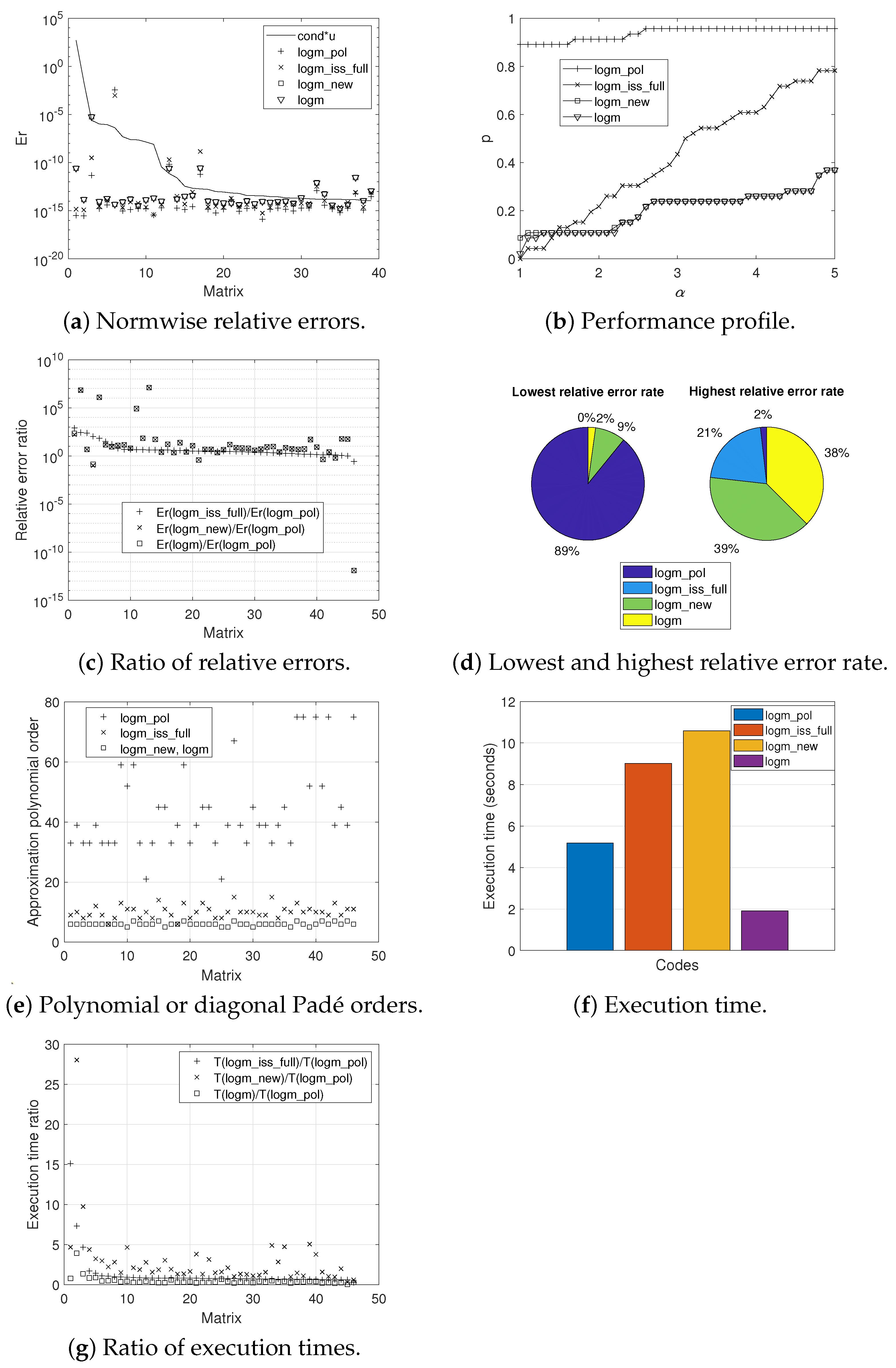
Graphically, Figure 1, Figure 2 and Figure 3 provide the results obtained according to the experiments carried out for each of the sets of matrices. More in detail, the normwise relative errors (a), the performance profiles (b), the ratio of the relative errors (c), the lowest and highest relative error rates (d), the polynomial or diagonal Padé orders (e), the execution times (f), and the ratio of the execution times (g) for the four codes analyzed can be appreciated.

Figure 1.
Experimental results for Set 1.
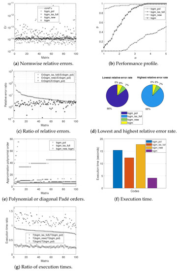
Figure 2.
Experimental results for Set 2.

Figure 3.
Experimental results for Set 3.
Figure 1a, Figure 2a and Figure 3a illustrate the normwise relative errors assumed by each of the codes when calculating the logarithm of the different matrices that comprise each of the sets. The solid line that appears in them depicts the function , where (or ) represents the condition number of the matrix logarithm function ([1], Chapter 3) and u is the unit round off. The numerical stability of each method is evidenced if its errors are not much higher than this solid line. The matrices were ordered by decreasing value of .
Roughly speaking, logm_pol obtained the lowest error values for most of the test matrices, whereas the top values corresponded to logm_iss_full, for Sets 1 and 2, or to logm_new and logm, for Set 3. Indeed, in the case of the first two sets, the vast majority of errors incurred by logm_pol are below the continuous line, while those of logm_new and logm are around this line and, in the case of logm_iss_full, clearly above it. The results provided by logm_new and logm were identical in the different experiments performed, with the exception of Set 3, where they were very similar. With regard to Set 3, the high condition number of the logarithm function for some test matrices meant that the maximum relative error committed by logm_pol punctually reached in one case the order of , closely followed by the error recorded by logm_iss_full. Nevertheless, for this third set of matrices and except for a few concrete exceptions, all methods provided results whose errors are usually located below the line.
Accordingly, these results showed that the numerical methods, on which the different codes were based, are stable, especially in the case of Taylor and its implementation in the logm_pol function, whose relative errors, as mentioned before, are always positioned in lowest positions on the graphs, thus delivering excellent results. It should be clarified that Matrices 19, 21, 23, 27, 51, and 52 from the MCT and Matrix 17 from the EMP are not plotted in Figure 3a because of the excessive condition number of the logarithm function, although it was taken into account in all other results.
Figure 1b, Figure 2b and Figure 3b trace the performance profile of the four codes where, on the x-axis, takes values from 1–5 with increments of 0.1. Given a specific value for the coordinate, the corresponding amount p on the y-axis denotes the probability that the relative error committed by a particular algorithm is less than or equal to -times the smallest relative error incurred by all of them.
In consonance with the results given in Table 5, the performance profiles showed that logm_pol was the most accurate function for the three matrix sets. In the case of the matrices belonging to the first two sets, the probability reached practically 100% in most of the figures, while it tended to be around 95% for the matrices that comprised the third set. Regarding the other codes, logm_new and logm offered practically identical results in accuracy, with a few more noticeable differences in the initial part of Figure 3b in favor of logm_new. On the other hand, logm_iss_full was significantly surpassed by logm_new and logm in Sets 1 and 2, with the opposite being true for Set 3, although in a more discrete manner.
The ratios in the normwise relative errors between logm_pol and the other tested codes are presented, in decreasing order according to Er(logm_iss_full)/Er(logm_pol), in Figure 1c, Figure 2c and Figure 3c. For the vast majority of the matrices in Sets 1 and 2, the values plotted are always greater than one, which again confirmed the superiority in terms of accuracy of logm_pol over the other codes, especially for logm_iss_full. Similar conclusions can be extracted from the analysis of the results for Set 3, although, in this case, the improvement of logm_pol was more remarkable over logm_new and logm for a small group of matrices.
In the form of a pie chart, the percentage of matrices in our test battery in which each method yielded the smallest or the largest normwise relative error over the other three ones is displayed in Figure 1d, Figure 2d and Figure 3d. Thus, on the positive side, logm_pol resulted in the lowest error in 94%, 86%, and 89% of the cases for, respectively, each of the matrix sets. Additionally, logm_pol never gave the most inaccurate result in the first two matrix sets and only gave the worst result in 2% of the matrices in Set 3. As can be seen, logm_iss_full gave the highest relative errors in 94% and 88% of the matrices correspondingly belonging to Set 1 and Set 2. On the contrary, the highest error rates were shared between logm_new and logm in Set 3.
The value of parameter m, or, in other words, the Taylor approximation polynomial order, in the case of logm_pol, or the Padé approximant degree, in the case of logm_iss_full, logm_new, and logm, is shown in Figure 1e, Figure 2e and Figure 3e, respectively, for the three sets. It should be clarified that the value and meaning of m is not comparable between logm_pol and the rest of the codes. Additionally, and for the three matrix sets, Table 6 collects those values of m, together with those ones of s, i.e., the number of matrix square roots computed, in the form of maxima, minima, means, and medians. Whereas the logm_pol function always required values of m much higher than the others, the values of s were more similar among the different codes, always reaching the smallest values on average in the case of logm_pol. Consequently, logm_pol needed to calculate a lower number of square roots compared to those required by the other codes. Moreover, it should be pointed out that logm_iss_full, logm_new, and logm were forced to use an atypically high value of s for a few matrices in Set 3. In all the experiments performed, logm_new and logm always employed an identical value of m and s.
Table 6.
Minimum, maximum, mean, and median values for the parameters m and s reached by logm_pol, logm_iss_full, logm_new, and logm for Sets 1–3, respectively.
On the other hand, Figure 1f, Figure 2f and Figure 3f and Table 7 inform us about the execution times spent by the different codes analyzed on computing the logarithm of all the matrices that constituted our testbed. To obtain these overall times, the runs were launched six times, discarding the first one and calculating the average time among the others. As we can appreciate, logm was always the fastest function, followed by logm_iss_full, for Sets 1 and 2, or by logm_pol, for Set 3. In contrast, logm_new always invested the longest time for our three experiments. Numerically speaking, and according to the times recorded for Set 3, logm_pol was 1.74- and 2.04-times faster than logm_iss_full and logm_new, respectively. This notwithstanding, logm_pol and the other codes were clearly outperformed by logm, whose speed of execution in computing the logarithm of this third set of matrices was 2.71-times higher than that of logm_pol.
Table 7.
Execution time (T), in seconds, corresponding to logm_pol, logm_iss_full, logm_new, and logm for computing matrices in the three sets.
In more detail, Figure 1g, Figure 2g and Figure 3g provide the ratio between the computation time of the other codes and logm_pol, individually for each of the matrices, in a decreasing order consistent with the factor T(logm_iss_full)/T(logm_pol). As an example, for Set 3, this ratio took values from 0.28 to 15.11 for logm_iss_full, from 0.32 to 28.03 for logm_new, and from 0.05 a 3.93 for logm.
Lastly, it is worth mentioning that, after performing the pertinent execution time profiles, it could be appreciated that much of the time spent by all the codes was involved in the square root computation. Indeed, observe that logm resulted in better execution times than logm_new, despite being two codes that share a similar theoretical scheme. This was mainly due to two reasons: first, because the recursive approach that logm follows to compute the square root of a triangular matrix is much more efficient than that of logm_new; second, this is due to implementation issues since, among others, logm is composed of distinct built-in functions in charge of, for example, calculating the Schur form, solving the Sylvester equation, or solving systems of linear equations, resulting in a very cost-effective code that is not possible to beat in speed as long as all its improvements are not also implemented in its competitors.
4. Conclusions
In this paper, an algorithm to approximate the matrix logarithm was designed. It uses recent matrix polynomial evaluation formulas corresponding to the Taylor series expansion of the logarithm function, which offers a lower computational cost than the Paterson–Stockmeyer method, but similar accuracy. From this algorithm, two MATLAB codes, according to relative forward or backward error analyses, were implemented. They were initially compared with each other and subsequently with MATLAB Codes 4.1 and 5.2 from [32], as well as with the logm built-in MATLAB function. For that, a testbed composed of three distinct types of matrices was used. The numerical results showed that the new Taylor-based codes are usually more accurate than the other state-of-the-art ones, with an intermediate execution time among all of them.
Author Contributions
Conceptualization, J.S., J.I. and E.D.; methodology, J.S., J.I., J.M.A. and E.D.; software, J.S., J.I., J.M.A. and P.R.; validation, J.M.A. and P.R.; formal analysis, J.S. and J.I.; investigation, J.S., E.D., J.M.A. and J.I.; writing—original J.S., J.I., E.D., P.R. and J.M.A.; writing—review and editing, J.S., J.I., E.D., P.R. and J.M.A. All authors read and agreed to the published version of the manuscript.
Funding
This research was funded by the European Regional Development Fund (ERDF) and the Spanish Ministerio de Economía y Competitividad Grant TIN2017-89314-P.
Institutional Review Board Statement
Not applicable.
Informed Consent Statement
Not applicable.
Data Availability Statement
Not applicable.
Conflicts of Interest
The authors declare no conflict of interest.
References
- Higham, N.J. Functions of Matrices: Theory and Computation; Society for Industrial and Applied Mathematics: Philadelphia, PA, USA, 2008. [Google Scholar]
- Miyajima, S. Verified computation for the matrix principal logarithm. Linear Algebra Its Appl. 2019, 569, 38–61. [Google Scholar] [CrossRef]
- Heßelmann, A.; Görling, A. Random phase approximation correlation energies with exact Kohn-Sham exchange. Mol. Phys. 2010, 108, 359–372. [Google Scholar] [CrossRef]
- Zachos, C.K. A classical bound on quantum entropy. J. Phys. A Math. Theor. 2007, 40, F407. [Google Scholar] [CrossRef]
- Schenk, T.; Richardson, I.; Kraska, M.; Ohnimus, S. Modeling buckling distortion of DP600 overlap joints due to gas metal arc welding and the influence of the mesh density. Comput. Mater. Sci. 2009, 46, 977–986. [Google Scholar] [CrossRef]
- Horenko, I.; Schütte, C. Likelihood-based estimation of multidimensional Langevin models and its application to biomolecular dynamics. Multiscale Model. Simul. 2008, 7, 731–773. [Google Scholar] [CrossRef] [Green Version]
- Han, I.; Malioutov, D.; Shin, J. Large-scale log-determinant computation through stochastic Chebyshev expansions. In Proceedings of the International Conference on Machine Learning, PMLR, Lille, France, 6–11 July 2015; pp. 908–917. [Google Scholar]
- Huang, Z.; Van Gool, L. A Riemannian network for SPD matrix learning. In Proceedings of the AAAI Conference on Artificial Intelligence, San Francisco, CA, USA, 4–9 February 2017; Volume 31, pp. 2036–2042. [Google Scholar]
- Dong, K.; Eriksson, D.; Nickisch, H.; Bindel, D.; Wilson, A.G. Scalable log determinants for Gaussian process kernel learning. In Proceedings of the 31st International Conference on Neural Information Processing Systems, Long Beach, CA, USA, 4–9 December 2017; pp. 6330–6340. [Google Scholar]
- Fitzsimons, J.; Granziol, D.; Cutajar, K.; Osborne, M.; Filippone, M.; Roberts, S. Entropic trace estimates for log determinants. In Machine Learning and Knowledge Discovery in Databases; Springer: Cham, Switzerland, 2017; pp. 323–338. [Google Scholar]
- Williams, P.M. Matrix logarithm parametrizations for neural network covariance models. Neural Netw. 1999, 12, 299–308. [Google Scholar] [CrossRef]
- Grindrod, P.; Higham, D.J. A dynamical systems view of network centrality. Proc. R. Soc. A Math. Phys. Eng. Sci. 2014, 470, 20130835. [Google Scholar] [CrossRef] [Green Version]
- Israel, R.B.; Rosenthal, J.S.; Wei, J.Z. Finding generators for Markov chains via empirical transition matrices, with applications to credit ratings. Math. Financ. 2001, 11, 245–265. [Google Scholar] [CrossRef]
- Singer, B.; Spilerman, S. The representation of social processes by Markov models. Am. J. Sociol. 1976, 82, 1–54. [Google Scholar] [CrossRef] [Green Version]
- Ossikovski, R.; De Martino, A. Differential Mueller matrix of a depolarizing homogeneous medium and its relation to the Mueller matrix logarithm. JOSA A 2015, 32, 343–348. [Google Scholar] [CrossRef] [PubMed]
- Ramézani, H.; Jeong, J. Non-linear elastic micro-dilatation theory: Matrix exponential function paradigm. Int. J. Solids Struct. 2015, 67, 1–26. [Google Scholar] [CrossRef]
- Rossignac, J.; Vinacua, Á. Steady affine motions and morphs. ACM Trans. Graph. (TOG) 2011, 30, 1–16. [Google Scholar] [CrossRef]
- Lastman, G.; Sinha, N. Infinite series for logarithm of matrix, applied to identification of linear continuous-time multivariable systems from discrete-time models. Electron. Lett. 1991, 27, 1468–1470. [Google Scholar] [CrossRef]
- Crouch, P.; Kun, G.; Leite, F.S. The De Casteljau algorithm on Lie groups and spheres. J. Dyn. Control. Syst. 1999, 5, 397–429. [Google Scholar] [CrossRef] [Green Version]
- Jiang, Y.L.; Xu, K. Frequency-limited reduced models for linear and bilinear systems on the Riemannian manifold. IEEE Trans. Autom. Control 2020. [Google Scholar] [CrossRef]
- Jafari, A.; Fiétier, N.; Deville, M.O. A new extended matrix logarithm formulation for the simulation of viscoelastic fluids by spectral elements. Comput. Fluids 2010, 39, 1425–1438. [Google Scholar] [CrossRef]
- Hulsen, M.A.; Fattal, R.; Kupferman, R. Flow of viscoelastic fluids past a cylinder at high Weissenberg number: Stabilized simulations using matrix logarithms. J.-Non-Newton. Fluid Mech. 2005, 127, 27–39. [Google Scholar] [CrossRef] [Green Version]
- Lee, H.; Ma, Z.; Wang, Y.; Chung, M.K. Topological Distances between Networks and Its Application to Brain Imaging. arXiv 2017, arXiv:1701.04171. [Google Scholar]
- Wang, X.; Schneider, T.; Hersche, M.; Cavigelli, L.; Benini, L. Mixed-Precision Quantization and Parallel Implementation of Multispectral Riemannian Classification for Brain-Machine Interfaces. In Proceedings of the 2021 IEEE International Symposium on Circuits and Systems (ISCAS), Daegu, Korea, 22–28 May 2021; pp. 1–5. [Google Scholar]
- Yu, P.L.; Wang, X.; Zhu, Y. High dimensional covariance matrix estimation by penalizing the matrix-logarithm transformed likelihood. Comput. Stat. Data Anal. 2017, 114, 12–25. [Google Scholar] [CrossRef]
- Grant Kirkland, W.; Sinha, S.C. Symbolic Computation of Quantities Associated With Time-Periodic Dynamical Systems. J. Comput. Nonlinear Dyn. 2016, 11, 041022. [Google Scholar] [CrossRef]
- Kenney, C.S.; Laub, A.J. A Schur–Fréchet Algorithm for Computing the Logarithm and Exponential of a Matrix. SIAM J. Matrix Anal. Appl. 1998, 19, 640–663. [Google Scholar] [CrossRef]
- Kenney, C.; Laub, A.J. Condition Estimates for Matrix Functions. SIAM J. Matrix Anal. Appl. 1989, 10, 191–209. [Google Scholar] [CrossRef] [Green Version]
- Higham, N.J. Evaluating Padé Approximants of the Matrix Logarithm. SIAM J. Matrix Anal. Appl. 2001, 22, 1126–1135. [Google Scholar] [CrossRef] [Green Version]
- Dieci, L.; Papini, A. Conditioning and Padé approximation of the logarithm of a matrix. SIAM J. Matrix Anal. Appl. 2000, 21, 913–930. [Google Scholar] [CrossRef]
- Cheng, S.H.; Higham, N.J.; Kenney, C.S.; Laub, A.J. Approximating the Logarithm of a Matrix to Specified Accuracy. SIAM J. Matrix Anal. Appl. 2001, 22, 1112–1125. [Google Scholar] [CrossRef] [Green Version]
- Al-Mohy, A.H.; Higham, N.J. Improved Inverse Scaling and Squaring Algorithms for the Matrix Logarithm. SIAM J. Sci. Comput. 2012, 34, C153–C169. [Google Scholar] [CrossRef] [Green Version]
- Al-Mohy, A.H.; Higham, N.J.; Relson, S.D. Computing the Fréchet Derivative of the Matrix Logarithm and Estimating the Condition Number. SIAM J. Sci. Comput. 2013, 35, C394–C410. [Google Scholar] [CrossRef] [Green Version]
- Fasi, M.; Higham, N.J. Multiprecision algorithms for computing the matrix logarithm. SIAM J. Matrix Anal. Appl. 2018, 39, 472–491. [Google Scholar] [CrossRef] [Green Version]
- Fasi, M.; Iannazzo, B. The Dual Inverse Scaling and Squaring Algorithm for the Matrix Logarithm; MIMS EPrint 2020.14; Manchester Institute for Mathematical Sciences, The University of Manchester: Manchester, UK, 2020. [Google Scholar]
- Cardoso, J.R.; Ralha, R. Matrix arithmetic-geometric mean and the computation of the logarithm. SIAM J. Matrix Anal. Appl. 2016, 37, 719–743. [Google Scholar] [CrossRef]
- Hale, N.; Higham, N.J.; Trefethen, L.N. Computing Aα, log(A), and related matrix functions by contour integrals. SIAM J. Numer. Anal. 2008, 46, 2505–2523. [Google Scholar] [CrossRef] [Green Version]
- Dieci, L.; Morini, B.; Papini, A. Computational techniques for real logarithms of matrices. SIAM J. Matrix Anal. Appl. 1996, 17, 570–593. [Google Scholar] [CrossRef] [Green Version]
- Tatsuoka, F.; Sogabe, T.; Miyatake, Y.; Zhang, S.L. Algorithms for the computation of the matrix logarithm based on the double exponential formula. J. Comput. Appl. Math. 2020, 373, 112396. [Google Scholar] [CrossRef] [Green Version]
- Golub, G.H.; Van Loan, C.F. Matrix Computations, 4th ed.; Johns Hopkins University Press: Baltimore, MD, USA, 2013. [Google Scholar]
- Sastre, J. Efficient evaluation of matrix polynomials. Linear Algebra Its Appl. 2018, 539, 229–250. [Google Scholar] [CrossRef]
- Sastre, J.; Ibáñez, J. Evaluation of Matrix Polynomials beyond the Paterson–Stockmeyer Method. Mathematics 2021, 9, 1600. [Google Scholar] [CrossRef]
- Sastre, J.; Ibáñez, J.; Defez, E. Boosting the computation of the matrix exponential. Appl. Math. Comput. 2019, 340, 206–220. [Google Scholar] [CrossRef]
- Ibáñez, J.; Alonso, J.M.; Sastre, J.; Defez, E.; Alonso-Jordá, P. Advances in the Approximation of the Matrix Hyperbolic Tangent. Mathematics 2021, 9, 1219. [Google Scholar] [CrossRef]
- Al-Mohy, A.H.; Higham, N.J. A New Scaling and Squaring Algorithm for the Matrix Exponential. SIAM J. Matrix Anal. Appl. 2009, 31, 970–989. [Google Scholar] [CrossRef] [Green Version]
- Ruiz, P.; Sastre, J.; Ibáñez, J.; Defez, E. High performance computing of the matrix exponential. J. Comput. Appl. Math. 2016, 291, 370–379. [Google Scholar] [CrossRef]
- Sastre, J.; Ibáñez, J.; Alonso-Jordá, P.; Peinado, J.; Defez, E. Fast Taylor polynomial evaluation for the computation of the matrix cosine. J. Comput. Appl. Math. 2019, 354, 641–650. [Google Scholar] [CrossRef]
- Higham, J.; Tisseur, F. A block algorithm for matrix 1-norm estimation, with an application to 1-norm pseudospectra. SIAM J. Matrix Anal. Appl. 2000, 21, 1185–1201. [Google Scholar] [CrossRef]
- Björck, A.; Hammarling, S. A Schur method for the square root of a matrix. Linear Algebra Its Appl. 1983, 52/53, 127–140. [Google Scholar] [CrossRef]
- Deadman, E.; Higham, N.J.; Ralha, R. Blocked Schur Algorithms for Computing the Matrix Square Root. In Applied Parallel and Scientific Computing; Manninen, P., Öster, P., Eds.; PARA 2012; Lecture Notes in Computer Science; Springer: Berlin/Heidelberg, Germany, 2013; Volume 7782, pp. 171–182. [Google Scholar]
- Higham, N.J. The Matrix Computation Toolbox. 2002. Available online: http://www.ma.man.ac.uk/higham/mctoolbox (accessed on 20 August 2021).
- Wright, T.G. Eigtool, Version 2.1. 2009. Available online: http://www.comlab.ox.ac.uk/pseudospectra/eigtool (accessed on 20 August 2021).

Publisher’s Note: MDPI stays neutral with regard to jurisdictional claims in published maps and institutional affiliations. |
© 2021 by the authors. Licensee MDPI, Basel, Switzerland. This article is an open access article distributed under the terms and conditions of the Creative Commons Attribution (CC BY) license (https://creativecommons.org/licenses/by/4.0/).