Mathematical Modelling of Turbulent Combustion of Two-Phase Mixtures of Gas and Solid Particles with a Eulerian–Eulerian Approach: The Case of Hydrogen Combustion in the Presence of Graphite Particles

Abstract

The numerical modelling of turbulent combustion of H₂–air mixtures with solid graphite particles is a challenging and key issue in many industrial problems including nuclear safety. This study presents a Eulerian–Eulerian model based on the resolution of the Navier–Stokes equations via large eddy simulation (LES) coupled with a system of ordinary differential equations (ODEs) of the detailed chemical kinetics to simulate the combustion of mixtures of gases and particles. The model was applied to predict the transient evolution of turbulent combustion sequences of mixtures of hydrogen, air and graphite particles under low concentration conditions. When applied to simulate lab-scale combustion experiments, the results showed a good agreement between experimental and numerical data using a detailed chemical kinetic model. Moreover, the model was able to predict some key experimental tendencies and revealed that the presence of a low concentration of graphite particles (~96 g/m³) in the scenario influenced the hydrogen combustion dynamics for mixtures of 20% (in volume) of hydrogen in air. Under these conditions, pressure levels reached at the walls of the sphere were increased and the combustion time was shortened. The results also showed the viability of using this kind of a model for obtaining global combustion parameters such as wall pressure evolution with time.

1. Introduction

Combustion of gas and particles mixtures is an issue of major interest in many different fields, including industrial combustors [1,2,3], pollutant emissions [4,5,6], solid propellants [7,8,9] or accident prediction and mitigation [10,11]. In this last field, prediction of particle behaviour with and without combustion is a key topic in nuclear power plants [12,13] as well as in fusion reactors such as the International Thermonuclear Experimental Reactor (ITER) [14,15]. In this case, the presence of particles might influence the combustion dynamics during a potential accident [16,17]. Therefore, it is of outmost importance to properly predict the effects of this type of turbulent combustion sequences in presence of solid particles.

Mathematical modelling of turbulent combustion requires a proper description of two key aspects: chemistry and turbulence. Large eddy simulation (LES) is a mathematical approach that provides a compromise between efficiency in terms of computational costs and detailed physical description of turbulence dynamics [18]. Several models are available for modelling turbulence at the subgrid scale (SGS) with LES. The Smagorinsky–Lilly [19] was the first one. It was developed for flows with homogeneous turbulence conditions. The wall-adapting local eddy model [20] is a common choice in the case of incompressible wall flows whereas the dynamic k_sgs equation model has been shown to behave relatively well in compressible flow conditions [21,22,23]. Regarding chemistry, it is important to use detailed kinetic models in order to predict several mechanisms such as ignition or quenching [24]. This is critical not only in the case of hydrogen combustion [25], but also in the case of other mixtures such as hydrogen and carbon. However, in this case, the number of detailed chemistry models available is still limited. Saxena and Williams [26] proposed a chemical kinetic mechanism for the combustion of hydrogen and carbon monoxide with 13 species and 30 reactions. They showed good results in their testing. Gibeling and Buggein [27] also developed a simplified model for the oxidation mechanism of carbon monoxide in the presence of hydrogen and oxygen. It considered nine species and 12 reactions and was used in propellant applications with satisfactory results. Zhuo et al. [28] also used a chemical kinetic model with eight species and 12 reactions for modelling carbon monoxide oxidation in the presence of hydrogen for propellant applications. In the case of mixtures of gases and particles, Bournot et al. [29] simulated a reactive two-phase flow with aluminium particles for base bleed applications. In this case, the chemistry model was very simple and only considered three species for the gas phase and two species for the particle phase. The turbulent nature of the flow was modelled in a statistical way. The results permitted to identify the global flow regimes of the problem. As for carbon particles, Chelliah et al. [30,31] studied the influence of particle porosity on the combustion of graphite particles in the presence of hydrogen under quasi-steady burning conditions. They relied on the chemical kinetic models proposed by Bradley [32] for nonporous graphite particles and by Yetter et al. [33] for CO–H₂O–O₂. A total of five reactions were considered for the solid carbon phase and 28 for the gas phase. A total of 13 species were considered in the problem. They confirmed the suitability of this kind of kinetic models with a comparison against experimental data. As for the modelling of particle behaviour in a turbulent gas flow, results of direct numerical simulations (DNS) for canonical problems permitted to give credit to less demanding numerical models such as LES. The Eulerian treatment when solving the governing continuum equations for averaged quantities of both phases is still limited with LES and DNS. There are just a few articles that have been devoted to the implementation of the Eulerian two-fluid approach in the framework of DNS or LES [34,35]. Yeh and Lei [36] used LES to investigate the motion of particles in isotropic and homogeneous shear flows. The generated particle-statistics by neglecting the subgrid scale (SGS) effects on particles showed that LES can successfully predict second-order statistics of particle motion. Similar results were obtained by other researchers [37,38,39,40].

As previously said, in the case of a combustion sequence within a dust-laden atmosphere in an industrial environment, a mining environment [10] or an accident scenario at a fission nuclear power plant [11] or the ITER fusion reactor [17], the presence of graphite particles might influence a potential hydrogen deflagration [41]. The sequence might degenerate into a dust explosion which might increase the accident impact [17]. Therefore, it is of major importance to properly predict the effects of this type of combustion sequences [41]. Previous works have assessed the effectiveness of LES models to predict the dynamics of premixed turbulent combustion of H₂–air mixtures [23]. In this work, we present a two-phase reacting model based on a Eulerian–Eulerian approach for both the gas and the solid phases. The model includes LES turbulence modelling and detailed kinetic schemes for the combustion chemistry of both the gas and the solid phases. These two approaches are not usually used in two-phase flow models that consider a Eulerian approach of both the gas and the solid phases. We explore the application of this model to a combustion two-phase flow problem with graphite particles in the presence of a premixed H₂–O₂–N₂ atmosphere. As commented above, this scenario is prototypical of several key industrial and safety problems. Specifically, we focus on the case of sequences in closed three-dimensional (3D) H₂ scenarios and investigate the effect of the presence of a low concentration of graphite dust particles in the combustion sequence. The comparison of combustion experiments from the literature with the numerical simulations permits to face the validation of the mathematical model proposed and evaluate its prediction capabilities. The article is structured as follows: firstly, the physical model and the numerical method used are presented. Later, the model is validated against ad-hoc experimental results obtained in a spherical bomb and the results obtained are discussed. Finally, some conclusions are drawn.

2. Mathematical Equations of the Model

2.1. A Two-Phase Flow Model for Mixtures of Gases and Solid Particles

The two-phase model used in this work relies on the hypothesis of highly diluted mixtures of gas and solid particles and considers a Eulerian–Eulerian approximation of the mass, momentum and energy conservation equations for both the gas phase and the solid phase. The system of equations also includes those corresponding to the concentration of the species of each phase. The gas phase is considered to be an ideal gas initially composed of a mixture of hydrogen and air (i.e., oxygen, nitrogen and argon). The solid phase was initially considered to be a monodisperse distribution of graphite (i.e., carbon, C) particles of 35 micrometres in diameter (Sauter median diameter) and particle density of 2160 kg/m³. During the combustion process, these species may react and generate additional species that will be detailed in the Combustion Model section.

In this case, the system of conservation equations averaged with the FAVRE approach (filtered local volume average of the equations) [42] was as follows:

$$\begin{array}{l}\frac{\partial {\rho }_g}{\partial t}+\overrightarrow{\nabla }·\left({\rho }_g{\overrightarrow{u}}_g\right)=\Gamma \\ \frac{\partial }{\partial t}\left({\rho }_g{\overrightarrow{u}}_g\right)+\overrightarrow{\nabla }·\left({\rho }_g{\overrightarrow{u}}_g\otimes {\overrightarrow{u}}_g+p\overline{I}\right)=\overrightarrow{\nabla }·\overline{\mathsf{\tau }}-{\overrightarrow{F}}_d+\Gamma {\overrightarrow{u}}_{\mathrm{p}}\\ \frac{\partial }{\partial t}\left({\rho }_g{E}_g\right)+\overrightarrow{\nabla }·\left({\rho }_g{\overrightarrow{u}}_g{H}_g-\overrightarrow{\nabla }·\left[\stackrel{=}{\mathsf{\tau }}·\overrightarrow{u}\right]+\overrightarrow{\nabla }·\overrightarrow{q}\right)=-{\overrightarrow{F}}_d·{\overrightarrow{u}}_g-\dot{Q_g}+\Gamma E_p+\dot{\frac{E_{\Delta }}{F}{Q}_{g,c}}\\ \frac{\partial \left({\rho }_g{Y}_{g,k}\right)}{\partial t}+\mathit{\nabla }·\left({\rho }_g{Y}_{g,k}{\overrightarrow{u}}_g\right)=S\mathit{\nabla }·\left(F{E}_{\Delta }{\rho }_{g}D\mathit{\nabla }{Y}_{g,k}\right)+\left(1-S\right)\mathit{\nabla }·\left({\rho }_g\left(D+D_{sgs}\right)\mathit{\nabla }{Y}_{g,k}\right)+\frac{E_{\Delta }}{F}{\dot{\omega }}_{g,k}\\ \mathrm{with}k=1, \dots , \mathrm{NGSP}-1\\ \frac{\partial \sigma }{\partial t}+\overrightarrow{\nabla }·\left(\sigma {\overrightarrow{u}}_p\right)=-\Gamma \\ \frac{\partial }{\partial t}\left(\sigma {\overrightarrow{u}}_p\right)+\overrightarrow{\nabla }·\left(\sigma {\overrightarrow{u}}_p\otimes {\overrightarrow{u}}_p\right)={\overrightarrow{F}}_d-\Gamma {\overrightarrow{u}}_{\mathrm{p}}\\ \frac{\partial }{\partial t}\left(\sigma E_p\right)+\overrightarrow{\nabla }·\left(\sigma {\overrightarrow{u}}_p{E}_p\right)={\overrightarrow{F}}_d{\overrightarrow{u}}_p+\dot{Q_g}-\Gamma E_{\mathrm{p}}+\dot{\frac{E_{\Delta }}{F}{Q}_{p,c}}\\ \frac{\partial }{\partial t}\left(\sigma Y_{p,k}\right)+\overrightarrow{\mathit{\nabla }}·\left(\sigma Y_{p,k}{\overrightarrow{u}}_p\right)={\dot{\omega }}_{p,k} k=1, \dots , NSSP-1\end{array}$$

(1)

with

$$\Gamma =\frac{E_{\Delta }}{F}{\displaystyle \sum }_{k=1}^{NPSP}{\dot{\omega }}_{p,\mathrm{k}}=-\frac{E_{\Delta }}{F}{\displaystyle \sum }_{k=1}^{NGSP}{\dot{\omega }}_{g,\mathrm{k}}$$

(2)

where the gas mixture is formed by NGSP gases and the solid mixture is formed by NPSP solids. The subscript $g$ indicates variables relating to the gas phase, while the subscript $p$ refers to the solid phase; ρ_g is the average gas density, ${\overrightarrow{u}}_m$ is the velocity of phase $m$ (i.e., gas phase “g” or solid particle phase “p”), $Y_{m,k}$ represents the mass fraction of species $k$ from phase $m$.

The hypothesis of a highly diluted mixture implies that void fraction ($\mathsf{\alpha }$) could be assumed to be near unity (α ≈ 1). Therefore, the concentration of particles is defined by $\sigma ={\rho }_g\left(1-\mathsf{\alpha }\right)$. $E_m$ and $H_m$ indicate, respectively, the total internal energy and the total enthalpy of phase $m$ (where “m” can be solid phase “p” or gas phase “g”). Mass fractions are defined so that if $NGSP$ is the number of components of the gas mixture and $NSSP$ is the number of solid species, the following relations are fulfilled:

$${\displaystyle \sum }_{k=1}^{NGSP}{Y}_{g,\mathrm{k}}=1; {\displaystyle \sum }_{k=1}^{NSSP}{Y}_{p,k}=1$$

(3)

Note that $\stackrel{=}{\mathsf{\tau }}$ represents the stress tensor and includes the turbulent (subgrid) stress terms, $\overrightarrow{\mathrm{q}}$ is the heat flux vector, Y_k is the mass fraction of species k, $\dot{{\mathsf{\omega }}_k}$ is the reaction rate of the k species and $D_k$ is the diffusion term of species k. Note that the expression of the species conservation equations includes the terms of the thickened flame model (TFM) used for modelling the turbulent combustion mechanism. These terms are explained in detail in the Combustion Model section of this work. Similarly, the energy conservation equation of the gas phase also includes the corresponding terms of the TFM in the transport terms (i.e., $\overrightarrow{\nabla }·[\stackrel{=}{\mathsf{\tau }}·\overrightarrow{\mathrm{u}}]+\overrightarrow{\nabla }·\overrightarrow{\mathrm{q}})$ in order to properly account for the heat and diffusion process in the turbulent combustion model.

$\dot{Q_c}$ is the heat released per unit of volume and time due to the chemical reactions, which is defined as follows:

$$\dot{Q_{g,c}}={\displaystyle \sum }_{k=1}^{NGSP}{\dot{\omega }}_{g,\mathrm{k}}·\Delta H_{fg,\mathrm{k}}; \dot{Q_{p,c}}={\displaystyle \sum }_{k=1}^{NSSP}\Delta H_{p,\mathrm{k}}.$$

(4)

where $\Delta H_{fm,\mathrm{k}}$ is the formation heat of species k.

In the model, the pressure effect on the solid phase is negligible and, therefore, solid particles can be considered to be incompressible. The gas–particle interaction was taken into account through source terms in the mass, momentum and energy equations. ${\overrightarrow{F}}_d$ is the gas–particle drag force, $\dot{Q_g}$ is the interfacial heat transfer rate, $\Gamma$ stands for the total mass exchange between phases, ${\dot{\omega }}_{m,k}$—for the species reaction rates. In the present approach, particle size was considered to be constant. This means that the model does not consider the change of particle diameter during the combustion process.

The equation of the state considered for the gas phase was as follows:

$$\mathrm{p}=\mathsf{\rho }\left({\displaystyle \sum }_{\mathrm{k}=1}^{NGSP}{\mathrm{Y}}_{\mathrm{k}}\frac{{\mathrm{R}}_{\mathrm{u}}}{{\mathrm{M}}_{\mathrm{k}}}\right)\mathrm{T}$$

(5)

where p denotes gas pressure, T—the gas temperature, R_u—the universal constant, M_k—the specific molar mass of the species k. Specific heats are temperature-dependent following the database by McBride et al. [43] and dynamic viscosity was considered to be temperature-dependent through Sutherland’s formula [44]:

$$\mathsf{\mu }=A_S\frac{T^{1/2}}{\left(1+T_S/T\right)}$$

(6)

Closure Equations for the Interphase Transport

The momentum exchange between the gas phase and the solid phase was taken into account by considering the drag force acting on a particle:

$${\overrightarrow{F}}_d=\frac{1}{2}{\rho }_g{C}_{d}A\left|{\overrightarrow{u}}_g-{\overrightarrow{u}}_p\right|\left({\overrightarrow{u}}_g-{\overrightarrow{u}}_p\right)$$

(7)

where C_d is the drag coefficient which is a function of the particle Reynolds number Re_p and A are the representative area of the particle [45]. Considering that the number of particles is σ/m_p, where m_p is the mass of a particle, and assuming spherical particles [46], the previous equation can be expressed as follows:

$${\overrightarrow{F}}_d=\frac{3\sigma }{4d_p{\rho }_p}{\rho }_g{C}_d\left|{\overrightarrow{u}}_g-{\overrightarrow{u}}_p\right|\left({\overrightarrow{u}}_g-{\overrightarrow{u}}_p\right)$$

(8)

The expression adopted in this work for the drag coefficient C_d is the one proposed by Otterman and Levine [47] and used by Miura and Glass [48] in their work:

C_d = 0.48 + 28Re_p^−0.85

(9)

where the Reynolds number for particles $R{e}_p=\frac{{\rho }_g{d}_p\left|{\overrightarrow{u}}_g-{\overrightarrow{u}}_p\right|}{{\mu }_g}$. The rate of the heat transferred from the gas to a particle at its surface, $\dot{Q_g}$, is as follows:

$$\dot{Q_g}=-\frac{\sigma }{m_p}\pi d_p{\mu }_g{c}_{pg}{\mathrm{Pr}}^{-1}\left(T_g-T_p\right)\mathrm{Nu}$$

(10)

where the Nusselt number (Nu) can be calculated as follows:

$$\mathrm{Nu}=2+0.6{\mathrm{Pr}}^{\frac{1}{3}}{\mathrm{Re}}^{\frac{1}{2}}$$

(11)

where Re is the gas Reynolds number, Pr—Prandtl number. This equation is valid for Re ≤ 50,000 according to Crowe et al. [45]. It was originally proposed by Knudsen and Katz [49] and has been used by different authors [47,48].

2.2. Model of the Chemical Kinetics

In order to evaluate precisely the rates of the chemical reactions present in the problem, a system of 33 ordinary differential equations (ODE) is considered and numerically solved to calculate the concentration of the different species at each timestep. In this work, the detailed chemical kinetics model used by Chelliah [30,31] was considered to describe the combustion of H₂ and solid carbon (C) in the presence of air. It was based on the chemical kinetic models proposed by Bradley [32] for nonporous graphite particles and Yetter et al. [33] for CO–H₂O–O₂. The model considered the following reactive species: C, CO, CO₂, HCO, H₂, H_, O₂, O, OH_, H₂O, H₂O₂ and HO₂. In accordance with the chemical kinetic models of Chelliah [30,31] and Yetter et al. [33] that were adopted in this work, it has been considered that atmospheric N₂ and Ar are nonreacting species that do not intervene in any of the reactions and do not undergo any oxidation process. This was done to maintain the integrity of the chemical models, without making any modifications that could alter their validity.

A total of five reactions were considered for the solid carbon phase (

Table 1. (a) Heterogenous rate constants for nonporous graphite oxidation (from Chelliah [30]). (b) Heterogenous rate constants for porous graphite oxidation (from Chelliah [30]). Here, ${\dot{s}}_i=W_i{c}_i{B}_i{T}^{{\alpha }_i}\exp \left(-E_i/RT\right)$ in kg/m²/s.

(a)
Reaction	i	Ai (1)	${\mathit{\alpha }}_{\mathit{i}}$	Ei (J/kmol)	$\dot{{\mathit{s}}_{\mathit{i}}}$ (kg/m2/s)
C+OH$\to$CO+H	1	3.56 × 10−3	−0.5	0.0	$\dot{s_1}=k_1{P}_{OH}$
C+O$\to$CO	2	6.56 × 10−3	−0.5	0.0	$\dot{s_2}=k_2{P}_O$
C+H2O$\to$CO+H2	3	4.74	0.0	2.878592 × 108	$\dot{s_3}=k_3{P}_{H_{2}O}^{0.5}$
C+CO2$\to$2CO	4	8.88 × 10−2	0.0	2.849304 × 108	$\dot{s_4}=k_4{P}_{C{O}_2}^{0.5}$
C+(1/2)O2$\to$CO	5	2.37 × 10−2	0.0	1.255200 × 108	$\dot{s_5}=\left\{\frac{k_{5}Y·P_{O_2}^{}}{1+k_6{P}_{O_2}^{}}+k_7{P}_{O_2}^{}\left(1-Y\right)\right\}$ where $Y={\left[1+\frac{k_8}{k_7{P}_{O_2}^{}}\right]}^{-1}$
	6	2.10 × 10−4	0.0	−1.715440 × 107
	7	5.28 × 10−4	0.0	6.359680 × 107
	8	1.79 × 102	0.0	4.058480 × 108
(b)
Reaction	i	Bi (1)	$\mathit{\alpha }$i	Ei (J/kmol)
C+OH$\to$CO+H	9	1.65	0.5	0.0
C+O$\to$CO	10	3.41	0.5	0.0
C+H2O$\to$CO+H2	11	6.00 × 107	0.0	2.690312 × 108
C+CO2$\to$2CO	12	6.0 × 107	0.0	2.690312 × 108
2C+O2$\to$2CO	13	2.2 × 106	0.0	1.799120 × 108

(a) ⁽¹⁾ The values of ${\mathrm{A}}_{\mathrm{i}}$ are in SI units: partial pressures are in Pa, ${\dot{s}}_i$ is in $\mathrm{kg}/\left({\mathrm{m}}^2·\mathrm{s}\right)$; ${\mathsf{\alpha }}_{\mathrm{i}}$ is dimensionless. (b) ⁽¹⁾ Units of ${\mathrm{B}}_{\mathrm{i}}\cdot {\mathrm{T}}^{{\mathsf{\alpha }}_{\mathrm{i}}}$ are s/m, and ${\mathsf{\alpha }}_{\mathrm{i}}$ is dimensionless.

). Two different mechanisms were tested in this study. One considered semiglobal heterogeneous surface reactions for nonporous graphite particles (Table 1a). The other considered semiglobal heterogeneous surface reactions for porous graphite particles (Table 1b). The mechanisms assumed that the primary product was CO and that each rate w < s independent of the others. The first assumption is known to be reasonable for high-temperature oxidation of graphite (i.e., temperature at the particle surface over 800 K) [50]. Note that in Table 1a, the rate $\dot{s_i}$ is expressed in terms of k_i = A_iT^αiexp(–E_i/RT), the partial pressure P_j is in Pa, T—in degrees Kelvin, whereas in Table 1b, the rate $\dot{s_i}$ is expressed in terms of $\dot{s_i}$ = W_i c_i B_iT^αiexp(–E_i/RT) in kg/m²/s. In this formula, B_iT^αi is in m/s, T—in degrees Kelvin. The gas phase homogeneous reaction mechanism of CO oxidation in the presence of H₂O considered here is the one proposed by Yetter et al. [33]. It consists of 12 species in 28 elementary reactions (

Table 2. Homogeneous rate constants of the CO/H₂O/O₂ reaction mechanism (from Chelliah, Chelliah et al. and Yetter et al. [30,31,33]) in the form $k_i=B_i{T}^{{\alpha }_i}\exp \left(-E_i/RT\right)$. Units are J, kmol, cm and K.

Step	Reaction	Bi (b)	αi (b)	Ei (J/kmol)
1	H + O2 = OH + O	1.91 × 1014	0.0	68,784,960
2	H2 + O = OH + H	5.13 × 104	2.67	26,317,360
3	H2 + OH = H2O + H	2.14 × 108	1.51	14,351,120
4	OH + OH = O+H2O	k = 5.46 × 1011	x	exp (0.00149·T)
5	H2 + M = H + H+M(a)	4.57 × 1019	−1.4	436,725,920
6	O + O+M = O2 + M(a)	6.17 × 1015	−0.5	0
7	H + O+M = OH + M(a)	4.68 × 1018	−1.0	0
8	H + OH + M = H2O + M(a)	2.24 × 1022	−2.0	0
9	H + O2 + M = HO2 + M(a)	4.76 × 1019	−1.42	0
10	HO2 + H = H2 + O2	6.61 × 1013	0.0	8,911,920
11	HO2 + H = OH + OH	17.0 × 1014	0.0	3,640,080
12	HO2 + O = OH + O2	1.74 × 1013	0.0	−1,673,600
13	HO2 + OH = H2O + O2	1.45 × 1016	−1.0	0
14	HO2 + HO2 = H2O2 + O2	3.02 × 1012	0.0	5,815,760
15	H2O2 + M = OH + OH + M(a)	1.20 × 1017	0.0	190,372,000
16	H2O2 + H = H2O + OH	1.00 × 1013	0.0	15,020,560
17	H2O2 + H = HO2 + H2	4.79 × 1013	0.0	33,262,800
18	H2O2 + O = HO2 + OH	9.55 × 106	2.0	16,610,480
19	H2O2 + OH = H2O + HO2	7.08 × 1012	0.0	5,983,120
20	CO + O+M = CO2 + M(a)	2.51 × 1013	0.0	−18,995,360
21	CO + O2 = CO2 + H	2.51 × 1012	0.0	199,534,960
22	CO + OH = CO2 + O	K = 6.75 × 1010	x	exp(0.000907·T)
23	CO + HO2 = CO2 + OH	6.03 × 1013	0.0	96,022,800
24	HCO + M = CO + H+M(a)	1.86 × 1017	−1.0	71,128,000
25	HCO + H = CO + H2	7.24 × 1013	0.0	0
26	HCO + O = CO + OH	3.02 × 1013	0.0	0
27	HCO + OH = CO + H2O	3.02 × 1013	0.0	0
28	HCO + O2 = CO + HO2	4.17 × 1012	0.0	0

^a The third-body efficiencies are H₂: 2.5, H₂O: 12.0, CO₂: 3.8, CO: 1.9. ^b Units of ${\mathrm{B}}_{\mathrm{i}}\cdot {\mathrm{T}}^{{\mathsf{\alpha }}_{\mathrm{i}}}$ are s/cm, and ${\mathsf{\alpha }}_{\mathrm{i}}$ is dimensionless.

). The rate constants for this mechanism were validated for a wide range of temperatures, pressures and reactant concentrations using shock tubes and flow reactor measurements. Following Yetter et al. [33], for high-temperature oxidation of CO, the non-Arrhenius rates recommended for reaction steps 4 and 22 were implemented.

For the species k, the total mass reaction rate ${\dot{\omega }}_k$ was defined as the contribution of all reactions:

$$\dot{{\mathsf{\omega }}_{\mathrm{k}}}={\displaystyle \sum }_{\mathrm{i}=1}^{\mathrm{NR}}\dot{{\mathsf{\omega }}_{\mathrm{k},\mathrm{i}}}{\mathsf{\delta }}_{\mathrm{k},\mathrm{i}}$$

(12)

where NR is the number of reactions. The Kronecker delta δ_k,i permits to take into account the reaction rate if species k was involved in reaction i. Finally, the heat released by the chemical reactions was modelled by the term $\dot{\mathrm{Q}}$, which included the contributions of all the reactions. It was defined as follows:

$$\dot{\mathrm{Q}}=-{\displaystyle \sum }_{\mathrm{i}=1}^{\mathrm{NGSP}}\dot{{\mathsf{\omega }}_{\mathrm{i}}}{\mathrm{H}}_{\mathrm{fm},\mathrm{i}}$$

(13)

where ΔH_fm,i is the heat of formation of species i.

2.3. A Detailed Turbulence Model

In order to describe the turbulence phenomena during the combustion in a realistic way in the model, LES approach was considered in this work. LES models make use of the filtered local volume-averaged conservation equations (FAVRE approach) [42] to solve the flow field, being the small-scale stresses solved with a subgrid-scale model [20] due to the low dependence of these scales on the geometry. In particular, the LES dynamic subgrid-scale kinetic energy model (LES k_sgs Eqn.) was used [21] in this work. This model was specially designed for compressible flows. In this model, the subgrid turbulent kinetic energy (k_sgs) is defined as followed:

$$k_{sgs}=\frac{1}{2}\left(\overline{u_k{u}_k}-{\overline{u}}_k{\overline{u}}_k\right)$$

(14)

It is calculated making use of the transport equation:

$$\rho \frac{\partial {\overline{k}}_{sgs}}{\partial t}+\rho \frac{\partial {\overline{u}}_j{\overline{k}}_{sgs}}{\partial x_j}=-{\tau }_{ij}\frac{\partial {\overline{u}}_i}{\partial x_j}-C_{\epsilon }\rho \frac{k_{sgs}{}^{3/2}}{{\Delta }_f}+\frac{\partial }{\partial x_j}\left(\frac{{\mathsf{\mu }}_t}{{\sigma }_k}\frac{\partial k_{sgs}}{\partial x_j}\right)$$

(15)

The subgrid-scale eddy viscosity is modelled as follows:

$${\mathsf{\mu }}_t=C_k\rho k_{sgs}{}^{1/2}{V}^{1/3}$$

(16)

where C_k is a constant and V^1/3 is the local grid scale calculated from the cell volume V in each cell as $V={\left(\Delta x\Delta y\Delta z\right)}^{}$ for inhomogeneous grids. The subgrid-scale turbulent stress tensor is calculated as follows:

$${\tau }_{ij}-\frac{2}{3}{k}_{sgs}{\delta }_{ij}=-2C_k{k}_{sgs}{}^{1/2} V^{1/3} dev\left(\overline{S_{ij}}\right)$$

(17)

where $dev\left(\overline{S_{ij}}\right)$ is the deviatoric component of the rate-of-strain tensor for the resolved scales. This way, the model relates the subgrid-scale stresses ${\tau }_{ij}$ to the large-scale strain-rate tensor $\overline{S_{ij}}$. This LES model showed good results when dealing with compressible flows [22] and gas reacting flows [18].

2.4. The Turbulent Combustion Model

The modelling of the combustion mechanism under the turbulent regime is a challenging physical problem that usually requires high computational costs as it must solve different time and spatial scales of a turbulent flame. In this work, the model chosen for modelling the turbulent combustion was the artificially thickened flame model (TFM). This model introduces an $\mathrm{F}$ factor in the energy and species equations of the gas phase that affects the thermal and molecular diffusivities (see Equation (1)). On the one hand, the $\mathrm{F}$ factor multiplies the pre-exponential factor of the kinetic equations; this permits to decrease the reaction rates by that factor. On the other hand, it increases the molecular diffusivity by the same factor. As the laminar flame speed is proportional to both magnitudes $(S_u\propto \sqrt{D\dot{\omega }})$, the model provides a flame which propagates at the same speed. Besides, the modelled flame is $\mathrm{F}$ times thicker as the laminar flame thickness is a function of $\left({\delta }_L^0\propto \sqrt{D/\dot{\omega }}\right)$. This way, the computational requirements of the mathematical model are relaxed, and less demanding grid sizes are required [51]. However, this approach modifies the physics of flame propagation since the Damköhler number is reduce [52]. This drawback is solved by taking into account the efficiency function $E_{\Delta }$ that takes into account the actual wrinkling of a turbulent flame by introducing subgrid wrinkling of the modelled flame. In this study, we used the efficiency function proposed by Charlette [53,54]. This function was calculated as follows:

$$E_{\Delta }={\left(1+min\left[\frac{\Delta }{{\delta }_L^0}-1, 0\right]·{\Gamma }_{\Delta }\left(\frac{\Delta }{{\delta }_L^0},\frac{u_{\Delta }^{\prime }}{S_L^0},R{e}_{\Delta }\right)\frac{u_{\Delta }^{\prime }}{S_L^0}\right)}^{\beta }$$

(18)

where ${\Gamma }_{\Delta }\left(\frac{\Delta }{{\delta }_L^0},\frac{u_{\Delta }^{\prime }}{S_L^0},R{e}_{\Delta }\right)$ is a function of the turbulent intensity $u_{\Delta }^{\prime }$ at the scale of the test filter scale $\Delta$, the subgrid-scale turbulent Reynolds $R{e}_{\Delta }$ and the laminar flame thickness ${\delta }_L^0$. The subgrid-scale turbulence intensity $u_{\Delta }^{\prime }$ was obtained from the obtained velocity resolved at the ${\Delta }_{mesh}$ scale as $u_{\Delta }^{\prime }=C_2{\Delta }_{mesh}{}^3\left|{\nabla }^2\left(\nabla \times \tilde{\mathit{u}}\right)\right|{\left(\frac{\Delta }{10\ast {\Delta }_{mesh}}\right)}^{1/3}$, with $C_2=2$. The Reynolds number at the subgrid scale was estimated as follows: $R{e}_{\Delta }=\frac{u_{\Delta }^{\prime }\Delta }{\nu }$. The flame laminar flame thickness at each cell was estimated following Charlette [53] procedure with the relationship ${\delta }_L^0\approx \frac{4·\nu }{S_L^0}$. Regarding the exponential factor, in this work, we used the fixed value of $\beta$ = 0.5 proposed by Charlette [53].

3. Numerical Methods

The finite volume approach was used to numerically solve the system of equations. After testing different numerical integration strategies, the numerical procedure that provided the best results was selected for the validation of the model. The numerical schemes chosen were AUSMup-HLLC Low Mach [55,56,57], Godunov Scheme for the gas phase and a flux-difference splitting scheme (Rusanov) [58] for the particle phase, both with a Van-Leer [59] TVD scheme. Time integration was performed with the classical four-stage Runge–Kutta scheme for the fluxes, inter-phase, turbulent and chemistry source terms. Thus, the fluxes and source terms involved in each transport equation were evaluated in multiple substeps per each fluid-convection timestep. Primitive variables were then reevaluated from the intermediate conservative variables evaluated for each Runge–Kutta slope evaluation substep. Fluxes, diffusive terms and source terms were then recalculated from the corresponding intermediate primitive values. Although a higher number of operations per timestep is needed, this scheme permitted to set a higher CFL number with a more stable fluid flow behavior during the simulation, avoiding the presence of numerical instabilities that might be encountered in the simulation results [7].

A second-order linear Gauss scheme was considered for spatial discretization, including gradient, divergence and Laplacian calculations. This numerical strategy was previously tested for hydrogen premixed turbulent combustion problems with good results [23]. Regarding the solid phase, a Rusanov scheme [58] was used to evaluate the convective fluxes in the conservation equations of the solid phase. This approach was previously validated for gas–particle combustion problems [7,8,14,16,17].

The integration of the ODE equation corresponding to chemistry source terms was a stiff problem difficult to solve in a cost-efficient way. After testing different strategies, an in situ adaptive tabulation method (ISAT) with ODE(SEULEX) integration [60,61] was used to solve the system of equations of the chemical kinetics of the gas phase and to estimate the reaction rate of the k^th species in the i^th reaction (${\dot{\omega }}_{k,i}$). ISAT is a method originally proposed for turbulent reacting flow simulations [60]. This method aims to approximate non-linear system solutions by means of a set of linear regressions of independent variables from a lookup tabulated database constructed dynamically with previous solutions (storage and retrieval method). Thus, it permits to reduce the number of ODE integrations for the chemistry set of ODE equations, being in the problem analyzed in this work one of the most computation-demanding tasks per integrated timestep. It has been reported that using this technique allows, under certain conditions, decreasing by three orders of magnitude the computer time required to compute the detailed chemistry in reacting flow computations [60]. This algorithm has been successfully applied in combustion chemistry problems involving up to 50 species [62] and was also used for premixed H₂–air combustion with detailed kinetics and LES–TFM modelling, similar approaches to the presented in this work [23,63]. A relative tolerance of 10⁻⁴ was set as the threshold for retraining the tabulated dataset. It is worth mentioning that this method is being extended to the applications other than the initially intended, especially for real-time predictive control [64] as an alternative to neural networks since it presents some advantages, e.g., it does not need training data before use.

The SEULEX ODE integration consists of a semi-explicit multistep method based on numerical extrapolation. An absolute tolerance 10⁻⁹ has been set, limiting to 1000 the maximum number of iterations per chemical gas integration.

Regarding the particle phase, a first-order implicit Euler scheme was used to integrate the chemistry equations with good results. Reaction rates for each timestep were evaluated using a sub-timestep (chemical timestep) in which each reaction rate for a given species and reaction is updated by the previous sub-timestep species concentrations. The temperatures used for evaluating the reaction rates were also updated from the last sub-timestep. An initial timestep of 10⁻¹² s was set, thus avoiding numerical fluctuations and divergences that may lead to nonphysical results.

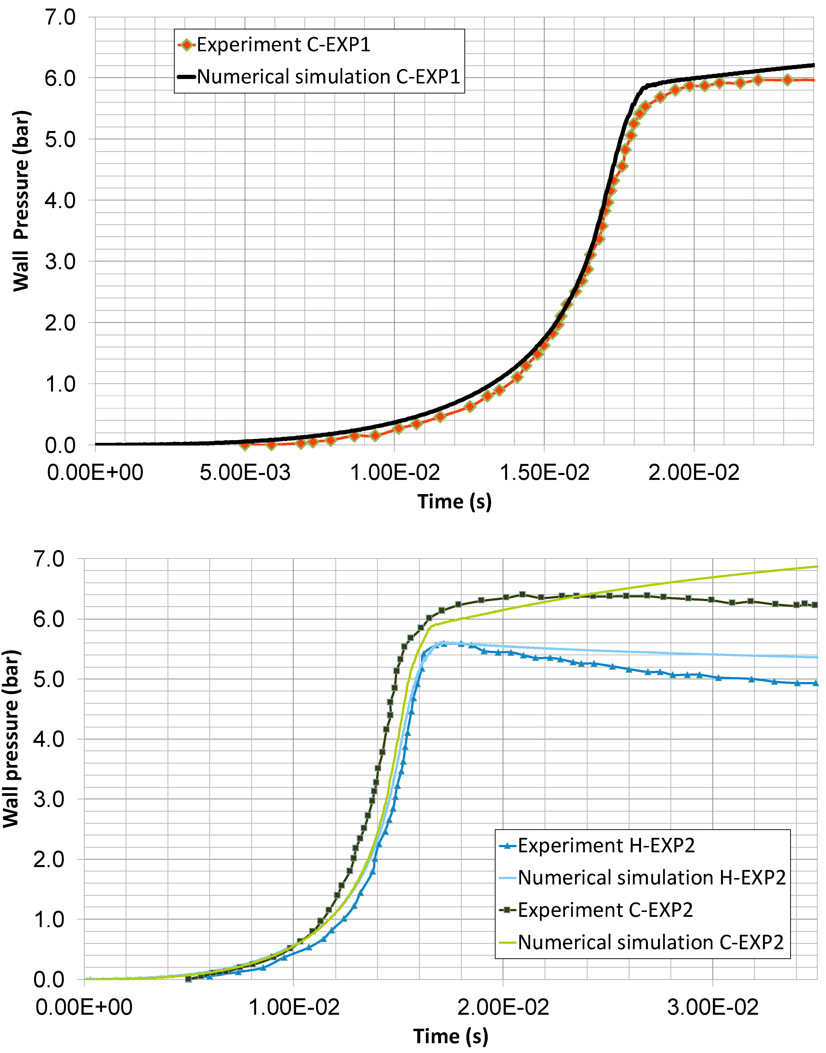
4. Results and Discussion

In the previous section, a two-phase flow model for turbulent combustion of gas and particles mixtures was presented. The use of LES, TFM and detailed kinetic schemes was explored as a way to take into account a realistic description of turbulence, flame wrinkling and reaction mechanisms in the turbulent combustion process. In order to validate the present model and evaluate its prediction capabilities, the experimental results from combustion tests presented by Sabard and Sabard et al. [65,66] were used as a reference benchmark. These experiments were performed at CNRS Orleans (France) and assessed the combustion of gas mixtures of H₂–O₂–N₂ and graphite (carbon) particles in a spherical bomb. The experimental facility consists of a spherical bomb with the internal radius of 125 mm equipped with different instrumentation including piezo-resistive wall pressure sensors, a Schlieren system, an electrical (spark) ignition system as well as a laser-induced ignition system (Figure 1). A detailed description of the experimental setup and methodology can be found in the works by Sabard and Sabard et al. [65,66,67]. During the experiments, different concentrations of C, H₂ and O₂ were introduced in the spherical bomb. The uncertainty in the volumetric composition of the gas mixture was below 0.3%, whereas the wall pressure measurements obtained had an experimental uncertainty smaller than 2%. The ignition of the mixture was generated with an electric spark between two electrodes. The initial pressure and temperature within the sphere were 1 bar and 298 K, respectively. The experimental conditions of the tests were as follows:

• Experiment 1 (C-EXP1): N₂/O₂ 3.76 and 20% H₂. Graphite powder concentration C(solid) = 94.1 g/m³;
• Experiment 2 (C-EXP2): N₂/O₂ 2.33 and 20% H₂. Graphite powder concentration C(solid) = 96.6 g/m³.

These experiments were simulated with the model presented in the previous section. The numerical domain defined for the simulations consists of an eighth part of a sphere with the radius of 125 mm. Thus, three different symmetry planes were considered. A grid sensitivity study was performed in order to check the potential influence of the spatial discretization simulated on the results. The results showed that there was a small influence of discretization in the radial direction when the mesh size was under 125 µm (i.e., 1000 radial elements). Independency of the opening angle was also assessed, reporting less than 0.3% in the variation of the maximum pressure and less than 0.115 ms differences in the rising time between the meshes with different angles. The final mesh size of 125 microns was used. Finer meshes had no influence on the chemistry mechanism and fluid fields. Regarding the initiation, it was assumed that an autoignition of the mixture which affected a small sphere with the radius of 2.5 mm initiated the sequence. This initiation was modelled as an addition of energy of 850 kJ/m³ applied to the ignition volume in 0.1 ms. This quantity of energy was enough to initiate a laminar flame in the domain.

The results of the experimental benchmark of the two-phase model are presented in Figure 2. The figure shows a comparison of the model prediction of pressure evolution at the wall of the spherical bomb with time with the experimental data obtained in Experiment 1 and Experiment 2. For the sake of comparison, an experiment performed without particles (called in the figure H-EXP2) was also included [66,67]. Its conditions were similar to Experiment 2 except for the presence of particles.

As shown, the two-phase approach proposed with LES and a detailed chemistry kinetic model was able to predict with good results the pressure evolution with time including the fast pressure rise found at the wall between 10 and 20 ms. As indicated in

Table 3. Comparison of the two-phase model prediction with experimental data. Prediction of the peak pressure and time of pressure rise.

Experiment 1	Experimental	Two-phase Model	Experiment 2	Experimental	Two-phase Model
Pmax (bar)	6.0	6.2	Pmax (bar)	6.4	6.9
Error, Pmax (%)	-	3.3	Error, Pmax (%)	-	7.8
trise (ms)	24.0	19.0	trise (ms)	20.9	17.1
Error, trise (%)	-	20.8	Error, trise (%)	-	18.2

, the model permitted to predict the maximum wall pressure (P_max) and the time lapsed to reach the maximum pressure (t_rise) with the relative error of 3.3% and 20.8%, respectively, for Experiment 1 and 7.8% (in P_max) and 18.2% (in t_rise) for Experiment 2. Taking into account the uncertainties linked with the ignition process (which are of the milliseconds order), the prediction of the time locus of the maximum pressure by the model could be considered satisfactory.

The model’s capacity to predict particle concentration effect on the combustion sequence can also be assessed by taking into account C-EXP2 and H-EXP2. As shown in Figure 2 (down), the model was able to predict the reduction of the maximum wall pressure when the particle concentration was reduced to zero. The model also showed a slight time displacement of the curve when the particle concentration was reduced. This displacement resulted in the increase of the combustion time but with approximately the same dP/dt. This experimental tendency was also well-captured by the model qualitatively. However, the experimental increase of the combustion time was larger than the one predicted by the model.

In general terms, Figure 2 shows a good agreement of the model with the experimental data. The main deviations between the simulations and the experiments are related to the final stage of the combustion process (i.e., for t > 20 ms) when the pressure level reached is maintained. These deviations can be related to the uncertainty found in the chemical model at high temperatures and to the influence of the graphite particle size. Therefore, the range of applicability of this model can be set on the basis of the conditions used in the validation, that is, H₂ concentration in the air of 20% for mixtures of N₂/O₂ between 2.33 and 3.76 at the initial ambient pressure and temperature, graphite particle size of the order of 35 microns and particle concentration between 0 and 97 g/m³.

As for the prediction of the combustion products,

Table 4. Comparison of the prediction of species concentration (%mol) in combustion gas products. Numerical prediction, experiments and the present model.

Experiment and Combustion Product Considered	COSILAB Numerical Prediction of the Combustion Products Considered (%mol) [66]	Experimental Measurements of the Combustion Products (%mol) [66]	Present Study: Two-Phase Model with the Porous Approach; (%mol) Prediction in Combustion Products	Present Study: Two-Phase Model with the Nonporous Approach; (%mol) Prediction in Combustion Products
Experiment 1, CO	15.44%	0%	0.22%	<0.0001%
Experiment 2, CO	11.57%	0%	1.46%	-
Experiment 1, H2O	10.76%	22.26%	20.77%	21.98%
Experiment 2, H2O	16.49%	22.29%	19.26%	-
Experiment 1, CO2	3.16%	4.34%	3.48%	0.012%
Experiment 2, CO2	8.23%	6.08%	5.26%	-

shows a comparison of the concentration of CO percentage in the combustion products estimated by this model and the one experimentally measured in the test C-EXP1 and C-EXP2 [66,67]. The table also includes the numerical prediction estimated with the Cosilab software for the same tests [66]. The results also permitted to compare the effect of different modelling approaches in the oxidation mechanism considered in the solid phase (porous vs. nonporous approximation). As shown, the mathematical model presented in this study provided better predictions of the CO composition in the combustion products than the Cosilab software in the case of both porous and nonporous modelling approaches. The table shows a good estimation of the porous model proposed, with deviations of less than 1.5% in the prediction of the volumetric percentage of CO in the combustion products and less than 0.1% in the case of the nonporous approach, whereas Cosilab provided a minimum deviation of 11%. The porous model provided results slightly closer to the experiments than the nonporous model in the prediction of gas combustion products. The comparison of the simulation results with both kinetic models (porous and nonporous) and its comparison with the experimental data of C-EXP1 and C-EXP2 also highlighted that the actual particle porosity was an important factor to predict transient subproducts of the combustion sequence. In fact, the consideration of the porous or the nonporous chemical kinetics model resulted in differences in the reaction rates of two order of magnitude. For example, in the case of the reactions C + 0.5 O₂ → CO and C + CO₂ → 2 CO, there were found differences of the order of 100 between both models. This was somehow expected as the particle porosity is directly linked to the actual effective particle surface which is directly linked to the reaction rates of the solid phase (Table 1). However, the actual particle porosity in industrial and safety problems commented upon above is usually unknown and must be considered from the practical point of view as an uncertainty factor of the model. All in all, it has to be remarked that regarding the prediction of P_max and t_rise both, the porous and nonporous chemical kinetics models presented the similar behaviour without remarkable quantitative differences in the dynamic evolution of wall pressure with time.

As for the applications of this model, it can be used to evaluate the efficiency of different strategies for tuning the products of the H₂–graphite combustion process to the desired conditions depending on the context.

In the nuclear safety context, a reduction of the combustion velocity and/or a quenching of the combustion process would be desirable. In this case, the strategy was to reduce the concentration of H₂ and/or O₂ in the scenario by promoting catalytic recombination that would reduce the probabilities of the deflagration-to-detonation transition. Under these circumstances, passive autocatalytic recombiners (PARs) are used to promote the reaction H₂ + O₂ → H₂O. In this case, there are undesirable subproducts in the H₂–graphite combustion whose concentration should be reduced to the minimum possible in order to avoid the poisoning of the catalyser. Specifically, because of the large sticking coefficient of CO compared to the other adsorbed species within a PAR and its high activation energy for desorption, the presence of CO in the mixture would poison the catalytic surface; this would prevent the desired recombination reaction in the PAR from occurring [68]. Besides, the lean limit concentration of hydrogen combustion decreases as the CO concentration increases and the flammable region widens for H₂–CO mixtures. Thus, CO is an undesirable by-product in the overall reaction [69]. Thus, in the safety context, the present model could be a useful tool to evaluate by means of numerical simulation the efficiency of different strategies used to mitigate the potential hazard during an accident sequence. For example, it can be applied in the prediction of accident sequences in ITER or in containment buildings of nuclear power plants, to adjust the parameters of mitigation systems such as N₂ injectors or passive autocatalytic recombiners.

In the industrial context, this numerical model can be applied in syngas combustors to evaluate potential strategies to reduce the concentration of H₂, CO and solid C at the exit of the combustor. For example, the development of IGCC technologies, involving gas-turbine combustion of syngas, derived, for instance, from air or O₂ gasification of pulverized coal, has recently promoted interest in studies of CO/H₂ combustion. In this case, this numerical model can be used to improve the efficiency of these combustors by predicting quenching, flame acceleration and/or spatial regions where the combustion process is inefficient and might lead to an increase in undesirable by-products.

5. Conclusions

In this work, we presented a numerical model for describing the turbulent combustion of two-phase flow mixtures of gas and particles. Specifically, we analysed the influence of the presence of solid carbon particles in the turbulent combustion of an H₂–air atmosphere. A two-phase model was proposed to describe this reacting flow with LES and detailed chemistry. The model proposed was benchmarked against experimental combustion data obtained in a spherical bomb. The results highlighted some significant specifics:

• In case of highly diluted mixtures of H₂–air and graphite particles, the benchmarked results showed that LES with a detailed chemistry model were found to be an appropriate engineering approach for analysing premixed turbulent combustion of graphite–H₂ mixtures.
• The validation against the experimental data show that the two-phase approach used in the present model based on the Eulerian–Eulerian approach seems to be accurate enough to afford this type of combustion sequences with highly diluted mixtures.
• Under the conditions studied, the model captured well the key tendencies linked to the presence of carbon particles of the microns order. In this sense, the model was able to predict that the presence of a low concentration of carbon particles (of the order of 96 g/m³) accelerated the combustion sequence, obtaining smaller combustion times than in the absence of particles and larger maximum wall pressure levels (of the order of 15%).
• Classical graphite and hydrogen detailed oxidation mechanisms [30,31,33] coupled with a Eulerian–Eulerian model provided good results in the prediction of combustion products under turbulent combustion conditions. Regarding graphite combustion, the porous oxidation model provided results closer to the experiments than the nonporous model.

Future work will face the extension of this model to other metal particles such as tungsten and to engineering applications of hydrogen turbulent combustion sequences.

References

1. Farid, M.M.; Jeong, H.J.; Kim, K.H.; Lee, J.; Kim, D.; Hwang, J. Numerical investigation of particle transport hydrodynamics and coal combustion in an industrialscale circulating fluidized bed combustor: Effects of coal feeder positions and coal feeding rates. Fuel 2017, 192, 187–200. [Google Scholar] [CrossRef]
2. Adamczyk, W.P.; Weçel, G.; Klajny, M.; Kozołub, P.; Klimanek, A.; Białecki, R.A. Modeling of particle transport and combustion phenomena in a large-scale circulating fluidized bed boiler using a hybrid Euler-Lagrange approach. Particuology 2014, 16, 29–40. [Google Scholar] [CrossRef]
3. Alattab, K.A.; Zainal, Z.A. Syngas production and combustion characteristics in a biomass fixed bed gasifier with cyclone combustor. Appl. Therm. Eng. 2017, 113, 714–721. [Google Scholar] [CrossRef]
4. Yang, B.; Wang, L.; Ning, L.; Zeng, K. Effects of pilot injection timing on the combustion noise and particle emissions of a diesel/natural gas dualfuel engine at low load. Appl. Therm. Eng. 2016, 102, 822–828. [Google Scholar] [CrossRef]
5. Goix, S.; Lévêque, T.; Xiong, T.; Schreck, E.; Baeza-Squiban, A.; Geret, F.; Uzug, G.; Austruy, A.; Dumat, C. Environmental and health impacts of fine and ultrafine metallic particles: Assessment of threat scores. Environ. Res. 2014, 133, 185–194. [Google Scholar] [CrossRef] [PubMed]
6. Benajes, J.; García, A.; Monsalve-Serrano, J.; Boronat, V. Gaseous emissions and particle size distribution of dualmode dualfuel dieselgasoline concept from low to full load. Appl. Therm. Eng. 2017, 120, 138–149. [Google Scholar] [CrossRef]
7. Otón-Martínez, R.A.; Monreal-González, G.; García-Cascales, J.R.; Vera-García, F.; Velasco, F.J.S.; Ramírez-Fernández, F.J. An approach formulated in terms of conserved variables for the characterisation of propellant combus-tion in internal ballistics. Int. J. Numer. Meth. Fluids 2015, 79, 394–415. [Google Scholar] [CrossRef]
8. Monreal-González, G.; Otón-Martínez, R.A.; Velasco, F.J.S.; García-Cascáles, J.R.; Ramírez-Fernández, F.J. One-Dimensional Modelling of Internal Ballistics. J. Energetic Mater. 2017, 35, 397–420. [Google Scholar] [CrossRef]
9. Kuo, K.K.; Summerfield, M. Fundamentals of Solid-Propellant Combustion, 90th ed.; American Institute of Aeronautics and Astronautics: New York, NY, USA, 1984. [Google Scholar]
10. Hamdan, M.; Qubbaj, A. Inhibition effect of inert compounds on oil shale dust explosion. Appl. Therm. Eng. 1998, 18, 221–229. [Google Scholar] [CrossRef]
11. Peng, W.; Chen, T.; Sun, Q.; Wang, J.; Yu, S. Preliminary experiment design of graphite dust emission measurement under accident conditions for HTGR. Nucl. Eng. Des. 2017, 316, 218–227. [Google Scholar] [CrossRef]
12. Herranz, L.; Del Prá, C.L.; Velasco, F.S. Preliminary steps toward assessing aerosol retention in the break stage of a dry steam generator during severe accident SGTR sequences. Nucl. Eng. Des. 2008, 238, 1392–1399. [Google Scholar] [CrossRef]
13. Raimond, E.; Clément, B.; Denis, J.; Guigueno, Y.; Vola, D. Use of Phébus FP and other FP programs for atmospheric radioactive release assessment in case of a severe accident in a PWR (deterministic and probabilistic approaches developed at IRSN). Ann. Nucl. Energy 2013, 61, 190–198. [Google Scholar] [CrossRef]
14. García-Cascales, J.R.; Otón-Martínez, R.A.; Sánchez-Velasco, F.J.; Vera-García, F.; Bentaiby, A.; Meynet, N. Advances in the characterisation of reactive gas and solid mixtures under low pressure conditions. Comput. Fluids 2014, 101, 64–87. [Google Scholar] [CrossRef]
15. Topilski, L.; Reyes, S. Accident Analysis Report—Vol. iii: Hypothetical Event Analysis; Technical Report ITER-D-2E2XAMv4.1, ITER Project; France, 2009. [Google Scholar]
16. García-Cascales, J.R.; Velasco, F.J.S.; Otón-Martínez, R.A.; Espín-Tolosa, S.; Bentaib, A.; Meynet, N.; Bleyer, A. Characterisation of metal combustion with DUST code. Fusion Eng. Des. 2015, 98–99, 2142–2146. [Google Scholar] [CrossRef]
17. Velasco, F.J.S.; Otón-Martínez, R.A.; García-Cascales, J.R.; Espín, S.; Meynet, N.; Bentaib, A. Modelling detonation of H2-O2-N2 mixtures in presence of solid particles in 3D scenarios. Int. J. Hydrog. Energy 2016, 41, 17154–17168. [Google Scholar] [CrossRef]
18. Pitsch, H. Large-eddy simulation of turbulent combustion. Annu. Rev. Fluid Mech. 2006, 38, 453–482. [Google Scholar] [CrossRef] [Green Version]
19. Lilly, D.K. A proposed modification of the Germano subgrid-scale closure method. Phys. Fluids A Fluid Dyn. 1992, 4, 633–635. [Google Scholar] [CrossRef]
20. Nicoud, F.; Ducros, F. Subgrid-Scale Stress Modelling Based on the Square of the Velocity Gradient Tensor. Flow Turbul. Combust. 1999, 62, 183–200. [Google Scholar] [CrossRef]
21. Chai, X.; Mahesh, K. Dynamic k-equation model for large eddy simulations of compressible flows. J. Fluid Mech. 2012, 699, 385–413. [Google Scholar] [CrossRef]
22. Nicolás-Pérez, F.; Velasco, F.J.S.; García-Cascales, J.R.; Otón-Martínez, R.A.; López-Belchí, A.; Moratilla, D.; Rey, F.; Laso, A. On the accuracy of RANS, DES and LES turbulence models for predicting drag reduction with Base Bleed technology. Aerospace Sci. Technol. 2017, 67, 126–140. [Google Scholar] [CrossRef]
23. Emami, S.; Mazaheri, K.; Shamooni, A.; Mahmoudi, Y. LES of flame acceleration and DDT in hydrogen–air mixture using artificially thickened flame approach and detailed chemical kinetics. Int. J. Hydrog. Energy 2015, 40, 7395–7408. [Google Scholar] [CrossRef]
24. Sánchez, A.L.; Williams, F.A. Recent advances in understanding of flammability characteristics of hydrogen. Prog. Energy Combust. Sci. 2014, 41, 1–55. [Google Scholar] [CrossRef]
25. Williams, F.A. Detailed and reduced chemistry for hydrogen autoignition. J. Loss Prev. Process. Ind. 2008, 21, 131–135. [Google Scholar] [CrossRef]
26. Saxena, P.; Williams, F.A. Testing a small detailed chemical-kinetic mechanism for the combustion of hydrogen and carbon monoxide. Combust. Flame 2006, 145, 316–323. [Google Scholar] [CrossRef]
27. Gibeling, H.; Buggeln, R. Reacting Flow Models for Navier-Stokes Analysis of Projectile Base Combustión; AIAA Paper No. 91-2077; AIAA: Reston, VA, USA, 1991. [Google Scholar]
28. Zhuo, C.; Feng, F.; Wu, X.; Liu, Q.; Ma, H. Numerical simulation of the muzzle flows with base bleed projectile based on dynamic overlapped grids. Comput. Fluids 2014, 105, 307–320. [Google Scholar] [CrossRef]
29. Bournot, H.; Daniel, E.; Cayzac, R. Improvements of the base bleed effect using reactive particles. Int. J. Therm. Sci. 2006, 45, 1052–1065. [Google Scholar] [CrossRef]
30. Chelliah, H. The influence of heterogeneous kinetics and thermal radiation on the oxidation of graphite particles. Combust. Flame 1996, 104, 81–94. [Google Scholar] [CrossRef]
31. Chelliah, H.K.; Makino, A.; Kato, I.; Araki, N.; Law, C.K. Modeling of graphite oxidation in a stagnation-point flow field using detailed homogeneous and semiglobal heterogeneous mechanisms with comparisons to experiments. Combust. Flame 1996, 104, 469–480. [Google Scholar] [CrossRef]
32. Bradley, D.; Dixon-Lewis, G.; Habik, S.E.; Mushi, E.M.J. Twentieth Symposium (International) on Combustion; The Combustion Institute: Pittsburgh, PA, USA, 1984; pp. 931–940. [Google Scholar]
33. Yetter, R.A.; Dryer, F.L.; Rabitz, H. A Comprehensive Reaction Mechanism For Carbon Monoxide/Hydrogen/Oxygen Kinetics. Combust. Sci. Technol. 1991, 79, 97–128. [Google Scholar] [CrossRef]
34. Druzhinin, O.A.; Elghobashi, S. On the decay rate of isotropic turbulence laden with micropaticles. Phys. Fluids 1999, 11, 602–610. [Google Scholar] [CrossRef]
35. Shotorban, B.; Balachandar, S. A Eulerian model for large-eddy simulation of concentration of particles with small Stokes numbers. Phys. Fluids 2007, 19, 118107. [Google Scholar] [CrossRef]
36. Yeh, F.; Lei, U. On the motion of small particles in a homogeneous isotropic turbulent flow. Phys. Fluids A Fluid Dyn. 1991, 3, 2571–2586. [Google Scholar] [CrossRef]
37. Simonin, O.; Deutsch, E.; Minier, J.P. Eulerian prediction of the fluid/particle correlated motion in turbulent two-phase flows. Flow Turbul. Combust. 1993, 51, 275–283. [Google Scholar] [CrossRef]
38. Wang, Q.; Squires, K. Large eddy simulation of particle-laden turbulent channel flow. Phys. Fluids 1996, 8, 1207–1223. [Google Scholar] [CrossRef]
39. Boivin, M.; Simonin, O.; Squires, K. On the prediction of gas–solid flows with two-way coupling using large eddy simulation. Phys. Fluids 2000, 12, 2080. [Google Scholar] [CrossRef]
40. Apte, S.; Mahesh, K.; Moin, P.; Oefelein, J. Largeeddy simulation of swirling particle-laden flows in a coaxialjet combustor. Int. J. Multiphase Flow 2003, 29, 1311–1331. [Google Scholar] [CrossRef]
41. Denkevits, A.; Dorofeev, S. Dust explosion hazard in ITER: Explosion indices of fine graphite and tungsten dusts and their mixtures. Fusion Eng. Des. 2005, 75–79, 1135–1139. [Google Scholar] [CrossRef]
42. Favre, A. Statistical equations of turbulent gases. In Problems of Hydrodynamic and Continuum Mechanics; SIAM: Philadelphia, PA, USA, 1969; pp. 231–266. [Google Scholar]
43. McBride, B.J.; Gordon, S.; Reno, M.A. Coefficients for Calculating Thermodynamic and Transport Properties of Individual Species; NASA: Washington, DC, USA, 1983. [Google Scholar]
44. Lii, W.S. The viscosity of gases and molecular force. Lond. Edinb. Dublin Philos. Mag. J. Sci. 1893, 36, 507–531. [Google Scholar] [CrossRef] [Green Version]
45. Crowe, C.T.; Schwarzkopf, J.D.; Sommerfeld, M.; Tsuji, Y. Multiphase Flows with Droplets and Particles; CRC Press: Boca Raton, FL, USA, 2011. [Google Scholar]
46. García-Cascales, J.R.; Vera-García, F.; Zueco-Jordán, J.; Bentaïb, A.; Meynet, N.; Vendel, J.; Perrault, D. Development of a IRSN code for dust mobilisation problems in ITER. Fusion Eng. Des. 2010, 85, 2274–2281. [Google Scholar] [CrossRef]
47. Otterman, B.; Levine, A.S. Analysis of Gas-Solid Particle Flows in Shock Tubes. AIAA J. 1974, 12, 579–580. [Google Scholar] [CrossRef]
48. Miura, H.; Glass, I.I. On dusty-gas shock tube. Proc. R. Soc. Lond. 1982, 382, 373–388. [Google Scholar]
49. Knudsen, J.G.; Katz, D.L.; Street, R.E. Fluid Dynamics and Heat Transfer. Phys. Today 1959, 12, 40–44. [Google Scholar] [CrossRef]
50. Laurendeau, N.M. Heterogeneous kinetics of coal char gasification and combustión. Prog. Energy Combust. Sci. 1978, 4, 221–270. [Google Scholar] [CrossRef]
51. Tabor, G.; Weller, H.G. Large Eddy Simulation of Premixed Turbulent Combustion Using Ξ Flame Surface Wrinkling Model. Flow Turbul. Combust. 2004, 72, 1–28. [Google Scholar] [CrossRef]
52. Poinsot, D.V.T. Theoretical and Numerical Combustion, 3rd ed.; RT Edwards, Inc.: West Bundaberg, Australia, 2012. [Google Scholar]
53. Charlette, F.; Meneveau, C.; Veynante, D. A power-law flame wrinkling model for LES of premixed turbulent combustion Part I: Non-dynamic formulation and initial tests. Combust. Flame 2002, 131, 159–180. [Google Scholar] [CrossRef]
54. Wang, G.; Boileau, M.; Veynante, D. Implementation of a dynamic thickened flame model for large eddy simulations of turbulent premixed combustion. Combust. Flame 2011, 158, 2199–2213. [Google Scholar] [CrossRef]
55. Liou, M.-S. A sequel to AUSM, Part II: AUSM+-up for all speeds. J. Comput. Phys. 2006, 214, 137–170. [Google Scholar] [CrossRef]
56. Liou, M.-S. A Sequel to AUSM: AUSM+. J. Comput. Phys. 1996, 129, 364–382. [Google Scholar] [CrossRef]
57. Koop, A.H. Numerical Simulation of Unsteady Three Dimensional Sheet Cavitation. Ph.D. Thesis, University of Twente, Enschede, The Netherlands, 2009. [Google Scholar] [CrossRef] [Green Version]
58. Rusanov, V. Calculation of interaction of non-steady shock waves with obstacles. J. Comput. Math. Phys. 1962, 1, 267–279. [Google Scholar]
59. Toro, E.F. Riemann Solvers and Numerical Methods for Fluid Dynamics; Springer: Berlin, Germany, 1997. [Google Scholar]
60. Pope, S. Computationally efficient implementation of combustion chemistry using in situ adaptive tabulation. Combust. Theory Model. 1997, 1, 41–63. [Google Scholar] [CrossRef]
61. Lu, L.; Pope, S.B. An improved algorithm for in situ adaptive tabulation. J. Comput. Phys. 2009, 228, 361–386. [Google Scholar] [CrossRef]
62. Hiremath, V.; Ren, Z.; Pope, S.B. Combined dimension reduction and tabulation strategy using ISAT–RCCE–GALI for the efficient implementation of combustion chemistry. Combust. Flame 2011, 158, 2113–2127. [Google Scholar] [CrossRef]
63. Nicolás-Pérez, F.; Velasco, F.J.S.; García-Cascales, J.R.; Otón-Martínez, R.A.; Bentaib, A.; Chaumeix, N. Evaluation of dif-ferent models for turbulent combustion of hydrogen-air mixtures. Large Eddy Simulation of a LOVA sequence with hy-drogen deflagration in ITER Vacuum Vessel. Fusion Eng. Des. 2020, 161, 111901. [Google Scholar] [CrossRef]
64. Hedengren, J.D.; Edgar, T.F. In Situ Adaptive Tabulation for Real-Time Control. Ind. Eng. Chem. Res. 2005, 44, 2716–2724. [Google Scholar] [CrossRef] [Green Version]
65. Sabard, J.; Chaumeix, N.; Bentaib, A. Hydrogen explosion in ITER: Effect of oxygen content on flame propagation of H2/O2/N2 mixtures. Fusion Eng. Des. 2013, 88, 2669–2673. [Google Scholar] [CrossRef]
66. Sabard, J. Etude de L’explosion de Mélanges Diphasiques: Hydrogène et Poussières. Ph.D. Thesis, Université d’Orléans, Orléans, France, 2013; pp. 185–221. [Google Scholar]
67. Sabard, J.; Goulier, J.; Chaumeix, N.; Mevel, R.; Studer, E.; Bentaib, A. Determination of explosion combustion parameters of H2/O2/N2 mixtures. In Proceedings of the International Symposium on Hazard, Prevention and Mitigation of Industrial Explosions (ISHPMIE), Cracov, Poland, 22–27 July 2012. [Google Scholar]
68. Jiménez, M.A.; Martín-Valdepeñas, J.M.; Martín-Fuertes, F.; Fernández, J.A. A detailed chemistry model for transient hy-drogen and carbon monoxide catalytic recombination on parallel flat Pt surfaces implemented in an integral code. Nucl. Eng. Des. 2007, 237, 460–472. [Google Scholar] [CrossRef] [Green Version]
69. Nuclear Energy Agency, Committee on the Safety of Nuclear Installations. Carbon Monoxide—Hydrogen Combustion Characteritics in Containment Conditions; Final Report, NEA/CSNI/R(2000)10; Nuclear Energy Agency: Paris, France, 2000. [Google Scholar]
Figure 1. Sketch of the spherical bomb ignition system and a wall pressure sensor.
Mathematics 09 02017 g001
Figure 2. Wall pressure evolution as a function of time. Comparison of numerical and experimental results for Experiment 1 (C-EXP1) (up) and Experiment 2 (C-EXP2) (down). “Wall pressure” represents relative pressure with respect to the atmospheric pressure.
Mathematics 09 02017 g002