A New Extended Model with Bathtub-Shaped Failure Rate: Properties, Inference, Simulation, and Applications

Abstract

Theoretical and applied researchers have been frequently interested in proposing alternative skewed and symmetric lifetime parametric models that provide greater flexibility in modeling real-life data in several applied sciences. To fill this gap, we introduce a three-parameter bounded lifetime model called the exponentiated new power function (E-NPF) distribution. Some of its mathematical and reliability features are discussed. Furthermore, many possible shapes over certain choices of the model parameters are presented to understand the behavior of the density and hazard rate functions. For the estimation of the model parameters, we utilize eight classical approaches of estimation and provide a simulation study to assess and explore the asymptotic behaviors of these estimators. The maximum likelihood approach is used to estimate the E-NPF parameters under the type II censored samples. The efficiency of the E-NPF distribution is evaluated by modeling three lifetime datasets, showing that the E-NPF distribution gives a better fit over its competing models such as the Kumaraswamy-PF, Weibull-PF, generalized-PF, Kumaraswamy, and beta distributions.

1. Introduction

Over the past three decades, the promising attention of researchers towards the development of new generalized models has increased to explore the hidden characters of baseline models. New generalized models open new horizons to address real-world problems and to provide an adequate fit to the complex and asymmetric random phenomena. Hence, various models have been constructed and studied in the literature. One of the simplest and most handy lifetime models induced in the statistical literature is the Lehmann Type I (L-I) and Type II models [1]. In the literature, the L-I model is most often discussed in favor of the power function (PF) distribution. The L-I model is simply the exponentiation of any baseline model, and it can be specified by the following cumulative distribution function (CDF):

$$F\left(x;\alpha ,\mathit{\xi }\right)=G^{\alpha }\left(x;\mathit{\xi }\right), \alpha >0, x\in ℝ.$$

Gupta et al. [2] utilized the L-I approach to define a generalized form of the exponential distribution. On the other hand, Cordeiro et al. [3] proposed a dual transformation to the L-I approach and defined the Lehmann Type II (L-II) G class of distributions, which is specified by the CDF:

$$F\left(x;\alpha ,\mathit{\xi }\right)=1-{\left(1-G\left(x;\mathit{\xi }\right)\right)}^{\alpha }, \alpha >0, x\in ℝ,$$

where $G\left(x;\mathit{\xi }\right)$ is the CDF of the arbitrary baseline model with a parametric vector $\xi$ and shape parameter $\alpha >0$.

The L-I and L-II approaches have been extensively utilized to propose more flexible and modified forms of classical models, due to their simple closed-form CDFs. The PF distribution is a simple form of the L-I distribution. The simplicity and usefulness of the PF distribution have attracted many researchers to study and explore its further extensions and applications in different applied areas. For example, Dallas [4] developed a relationship between the PF and Pareto distributions, Meniconi and Barry [5] adopted the PF distribution to model electronic components data, Chang [6] discussed the independence of record values based on the characterization of the PF distribution, Tavangar [7] characterized the PF distribution by dual generalized order statistics, Ahsanullah et al. [8] adopted the lower record values to characterize the PF distribution, Zaka et al. [9] discussed the estimation of the PF parameters via various estimation methods, and Shahzad et al. [10] discussed the estimation of the PF parameters via the trimmed L moments. Furthermore, some notable extensions of the PF distribution include, for example, the beta-PF [11], Weibull-PF [12,13], transmuted-PF [14], weighted-PF [15], Marshall–Olkin PF [16], transmuted generalized-PF [17], exponentiated transmuted-PF [18], and odd generalized exponential PF [19], and recently, Arshad et al. [20,21] developed a bounded bathtub-shaped failure rate PF model via L-II class, called the exponentiated-PF distribution.

The basic aim to carry out the present study is to develop a flexible bathtub-shaped failure rate model called the exponentiated new power function (E-NPF) distribution, which has some useful properties such as (i) its CDF, probability density function (PDF), and likelihood function are simple and easy to interpret; (ii) from the application perspective, this model is quite uncomplicated; (iii) its density and failure rate shapes follow the skewed and bathtub shapes; and (iv) this model provides a consistently better fit over its competitors.

Moreover, the E-NPF parameters are estimated using several classical methods of estimation. The comparisons and performance of these estimators have been explored via simulation results. Moreover, the maximum likelihood is adopted under type II censored samples to estimate the E-NPF parameters. Several articles have addressed the estimation of the model parameters using different estimators and compared them to determine the best estimation approach. For example, see [22,23,24,25] and the references therein.

This paper is arranged in the following sections. The proposed E-NPF model is developed in Section 2. Comprehensive studies on its mathematical and reliability characteristics are presented in Section 3. Estimations of the E-NPF parameters by eight estimation methods are presented in Section 4. Section 5 illustrates the simulation results by using eight estimation methods. Applications of the E-NPF model to three real datasets are discussed in Section 6 to illustrate its importance and flexibility. Some final conclusions are discussed in Section 7.

2. Materials and Methods

Iqbal et al. [26] studied a two-parameter model called the new power function (NPF) distribution which is specified by the following CDF:

$$F\left(x;\alpha ,\beta \right)=1-{\left(\frac{1-x}{1+\alpha x}\right)}^{\beta } ,$$

and its associated PDF reduces to

$$f\left(x;\alpha ,\beta \right)=\frac{\beta \left(1+\alpha \right){\left(1-x\right)}^{\beta -1}}{{\left(1+\alpha x\right)}^{\beta +1}} ,$$

where$x\in \left(0,1\right),$ $-1<\alpha <\infty ,\beta >0$ are the scale and shape parameters, respectively.

To this end, we define the E-NPF distribution that can model asymmetric and bathtub-shaped failure rate phenomena. For this, following Gupta et al. [2], we add up a shape parameter to the baseline NPF model. The newly added parameter advances the tail weight of the E-NPF density and starts providing a consistently better fit over its competitors.

A random variable $X$ is said to follow the E-NPF distribution, say $X~$E-NPF($\eta ,\zeta ,\theta$), if its CDF takes the form

$$F_{\mathrm{E}-\mathrm{NPF}}\left(x;\eta ,\zeta ,\theta \right)={\left(1-{\left(\frac{1-x}{1+\eta x}\right)}^{\zeta }\right)}^{\theta } ,$$

(1)

and its corresponding PDF reduces to

$$f_{\mathrm{E}-\mathrm{NPF}}\left(x;\eta ,\zeta ,\theta \right)=\frac{\theta \zeta \left(1+\eta \right)}{{\left(1+\eta x\right)}^2}{\left(\frac{1-x}{1+\eta x}\right)}^{\zeta -1}{\left(1-{\left(\frac{1-x}{1+\eta x}\right)}^{\zeta }\right)}^{\theta -1},$$

(2)

where$x\in \left(0,1\right),$ $-1<\eta <\infty ,$ is a scale and $\zeta ,\theta >0$ are the two shape parameters, respectively. The two special models of the E-NPF distribution are listed in

Table 1. Sub-models for different parameters.

Parameter	Model	Author(s)
$\theta =1$	NPF distribution	Iqbal et al. [22]
$\theta =1$, and $\eta =0$	L-II distribution	Lehmann-II [1]

.

3. Mathematical Properties

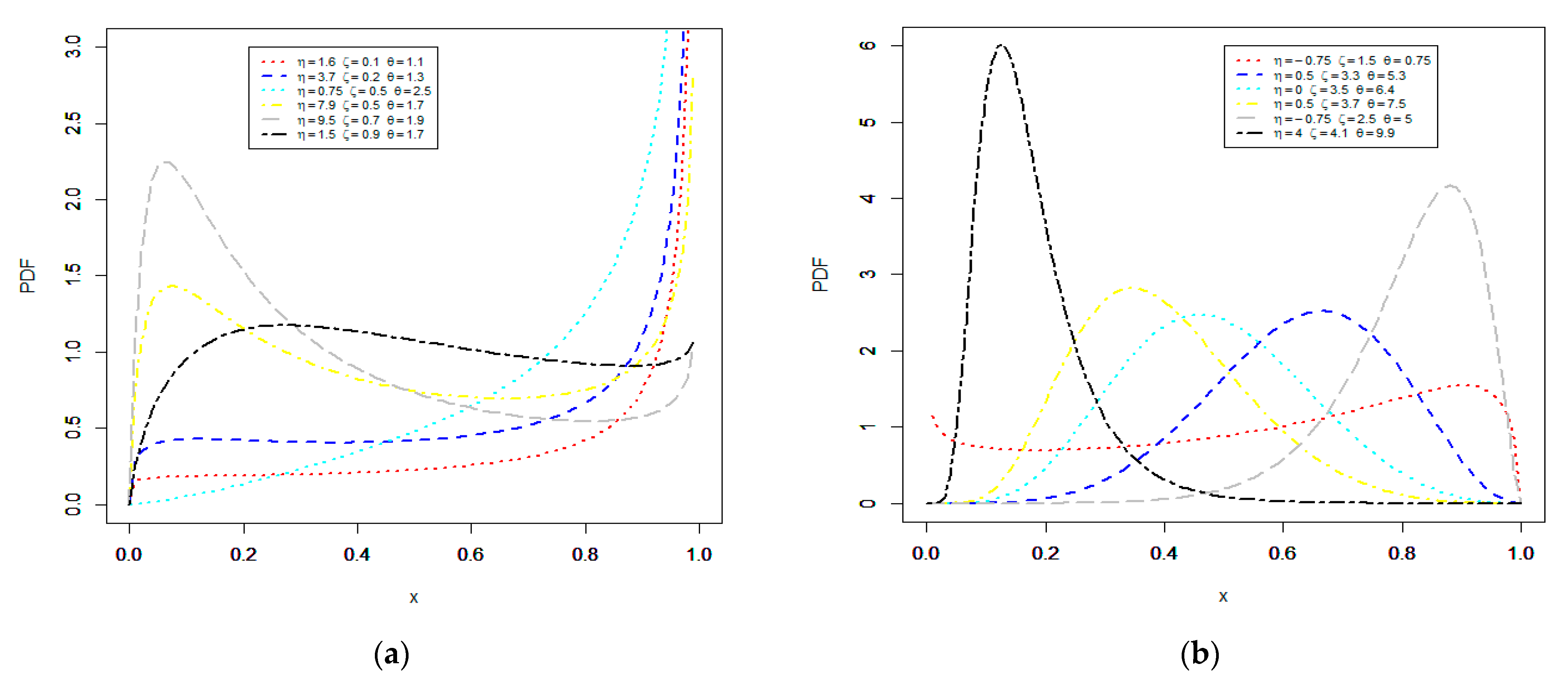
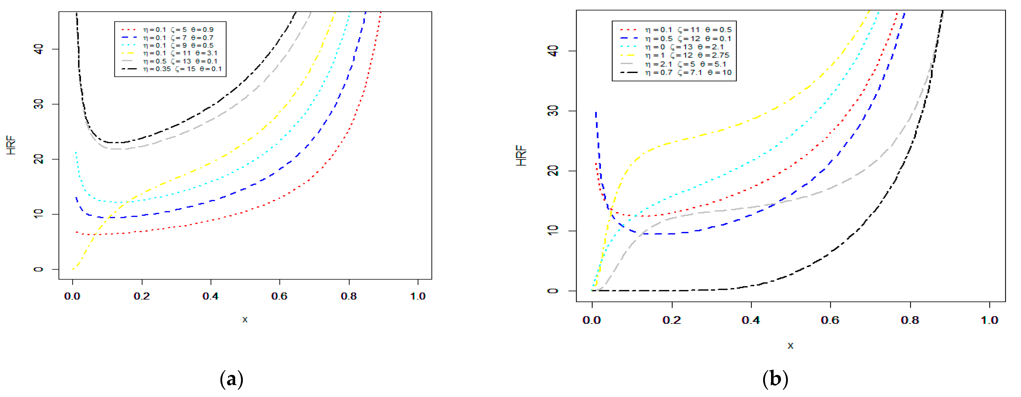
3.1. Shape

Several shapes for the E-NPF density and failure rate functions are displayed in Figure 1 and Figure 2 for various choices of the parameters. Note that the possible shapes of the PDF corresponding to the parameter $\eta$, which controls the scale of the distribution, along with the two shape parameters $\zeta$ and $\theta$, which control the shapes of the distribution, including increasing, symmetric, upside-down bathtub, decreasing, and J shapes. These shapes are presented in Figure 1a,b. Furthermore, Figure 2a,b presents the hazard rate function (HRF) shapes, including increasing, U, and bathtub shapes. These flexible HRF shapes are suitable for both the monotonic and non-monotonic hazard rate behaviors, which are most likely to appear in real-time situations (see Pu et al. [27] and Oluyede et al. [28]). Such kinds of shapes are often observed in non-stationary lifetime phenomena.

3.2. Linear Representation

Linear combination provides a simple way to explore the mathematical properties of the model. For this reason, binomial expansion is utilized. It is given as

$${\left(1-z\right)}^{\varphi -1}={\displaystyle \sum }_{j=0}^{\infty }{(-1)}^j\left(\begin{array}{c}\varphi -1\\ j\end{array}\right)z^j ,-1<z<1.$$

Infinite linear combinations of CDF and PDF in Equations (1) and (2) are given, respectively, by

$$F_{\mathrm{E}-\mathrm{NPF}}\left(x;\eta ,\zeta ,\theta \right)={\displaystyle \sum }_{i=0}^{\infty }{\displaystyle \sum }_{j=0}^{\infty }{\displaystyle \sum }_{k=0}^{\infty }{w}_{ijk}{x}^{j+k}$$

(3)

and

$$f_{\mathrm{E}-\mathrm{NPF}}\left(x;\eta ,\zeta ,\theta \right)=\zeta \theta \left(1+\eta \right){\displaystyle \sum }_{i=0}^{\infty }{\displaystyle \sum }_{j=0}^{\infty }{(-1)}^i\left(\begin{array}{c}\theta -1\\ i\end{array}\right)\left(\begin{array}{c}\alpha \\ j\end{array}\right){\left(\eta x\right)}^j{\left(1-x\right)}^{\zeta },$$

(4)

$$f_{\mathrm{E}-\mathrm{NPF}}\left(x;\eta ,\zeta ,\theta \right)=\zeta \theta \left(1+\eta \right){\displaystyle \sum }_{i=0}^{\infty }{\displaystyle \sum }_{j=0}^{\infty }{\displaystyle \sum }_{k=0}^{\infty }{v}_{ijk} x^{j+k},$$

(5)

where

$$\begin{array}{c}{w}_{ijk}={(-1)}^{i+k}{\eta }^j\left(\begin{array}{c}\theta \\ i\end{array}\right)\left(\begin{array}{c}-\zeta i\\ j\end{array}\right)\left(\begin{array}{c}\zeta i\\ k\end{array}\right), \\ v_{ijk}={(-1)}^{i+k}{\eta }^j\left(\begin{array}{c}\theta -1\\ i\end{array}\right)\left(\begin{array}{c}\alpha \\ j\end{array}\right)\left(\begin{array}{c}\beta \\ k\end{array}\right),\\ \mathrm{and} \alpha =-\zeta \left(1+i\right)-1, \beta =\zeta \left(1+i\right)-1.\end{array}$$

The expression in Equation (4) will be adopted in the forthcoming calculations of several mathematical properties of the E-NPF distribution.

3.3. Reliability Characteristics of the E-NPF Model

Analyzing and predicting the lifetime of a component are important roles in reliability engineering. Hence, some useful and well-established reliability measures are accessible in the literature.

The survival function of $X$, which represents the probability that a component will survive till time x, takes the form

$$S_{\mathrm{E}-\mathrm{NPF}}\left(x;\eta , \zeta ,\theta \right)=1-{\left(1-{\left(\frac{1-x}{1+\eta x}\right)}^{\zeta }\right)}^{\theta }.$$

(6)

In reliability theory, the function that measures the failure rate of a component in a particular period t is also referred to as the force of mortality or HRF. The HRF of the E-NPF distribution has the form

$$h_{\mathrm{E}-\mathrm{NPF}}\left(x;\eta ,\zeta ,\theta \right)=\frac{\theta \zeta \left(1+\eta \right){\left(1-x\right)}^{\zeta -1}{\left(1-{\left(\frac{1-x}{1+\eta x}\right)}^{\zeta }\right)}^{\theta -1}}{{\left(1+\eta x\right)}^2{\left(1+\eta x\right)}^{\zeta -1}\left(1-{\left(1-{\left(\frac{1-x}{1+\eta x}\right)}^{\zeta }\right)}^{\theta }\right)} .$$

(7)

It is well known that most mechanical parts/components of some systems follow a bathtub-shaped hazard rate phenomenon. The cumulative hazard rate (CHR) function is expressed by $H\left(x\right)=-\log \left(S\left(x\right)\right).$ The CHR function of X is given by

$$H_{\mathrm{E}-\mathrm{NPF}}\left(x;\eta ,\zeta ,\theta \right)=-lo\mathrm{g}\left(1-{\left(1-{\left(\frac{1-x}{1+\eta x}\right)}^{\zeta }\right)}^{\theta }\right).$$

(8)

The reverse HRF (RHRF) is expressed by $W\left(x\right)=f\left(x\right)/F\left(x\right).$ The RHRF of the E-NPF model takes the form

$$W_{\mathrm{E}-\mathrm{NPF}}\left(x;\eta ,\zeta ,\theta \right)=\frac{\theta \zeta \left(1+\eta \right){\left(1-x\right)}^{\zeta -1}}{{\left(1+\eta x\right)}^2{\left(1+\eta x\right)}^{\zeta -1}\left(1-{\left(\frac{1-x}{1+\eta x}\right)}^{\zeta }\right)}.$$

(9)

The Mills ratio (MR) is expressed by $M\left(x\right)=S\left(x\right)/f\left(x\right).$ The MR of $X$ reduces to

$$M_{\mathrm{E}-\mathrm{NPF}}\left(x;\eta ,\zeta ,\theta \right)=\frac{\left({\left(1+\eta x\right)}^{1+\zeta }\right)\left(1-{\left(1-{\left(\frac{1-x}{1+\eta x}\right)}^{\zeta }\right)}^{\theta }\right)}{\theta \zeta \left(1+\eta \right){\left(1-x\right)}^{\zeta -1}{\left(1-{\left(\frac{1-x}{1+\eta x}\right)}^{\zeta }\right)}^{\theta -1}}.$$

(10)

The odd function is expressed by $O\left(x\right)=F\left(x\right)/S\left(x\right)$ and it is defined, for the E-NPF model, by

$$O_{\mathrm{E}-\mathrm{NPF}}\left(x;\eta ,\zeta ,\theta \right)={\left({\left(1-{\left(\frac{1-x}{1+\eta x}\right)}^{\zeta }\right)}^{-\theta }-1\right)}^{-1}.$$

(11)

3.4. Limiting Behavior

The limiting behaviors of cumulative distribution, density, reliability, and hazard rate functions of the E-NPF distribution, which are defined, respectively, in Equations (1), (2), (6), and (7) at x$\to 0$ and x$\to 1$, are discussed in Propositions 1 and 2.

Proposition 1.

The limiting behaviors of functions (1), (2), (6), and (7) at x$\to 0$are, respectively, presented by

F_(E-NPF) (x)~0,
f_(E-NPF) (x)~θζ(1+η),
S_(E-NPF) (x)~1,
h_(E-NPF) (x)~0.

(12)

Proposition 2.

The limiting behaviors of functions (1), (2), (6), and (7) at x$\to 1$are, respectively, determined by

F_(E-NPF) (x)~1,
f_(E-NPF) (x)~0,
S_(E-NPF) (x)~0,
h_(E-NPF) (x)~Indeterminate.

(13)

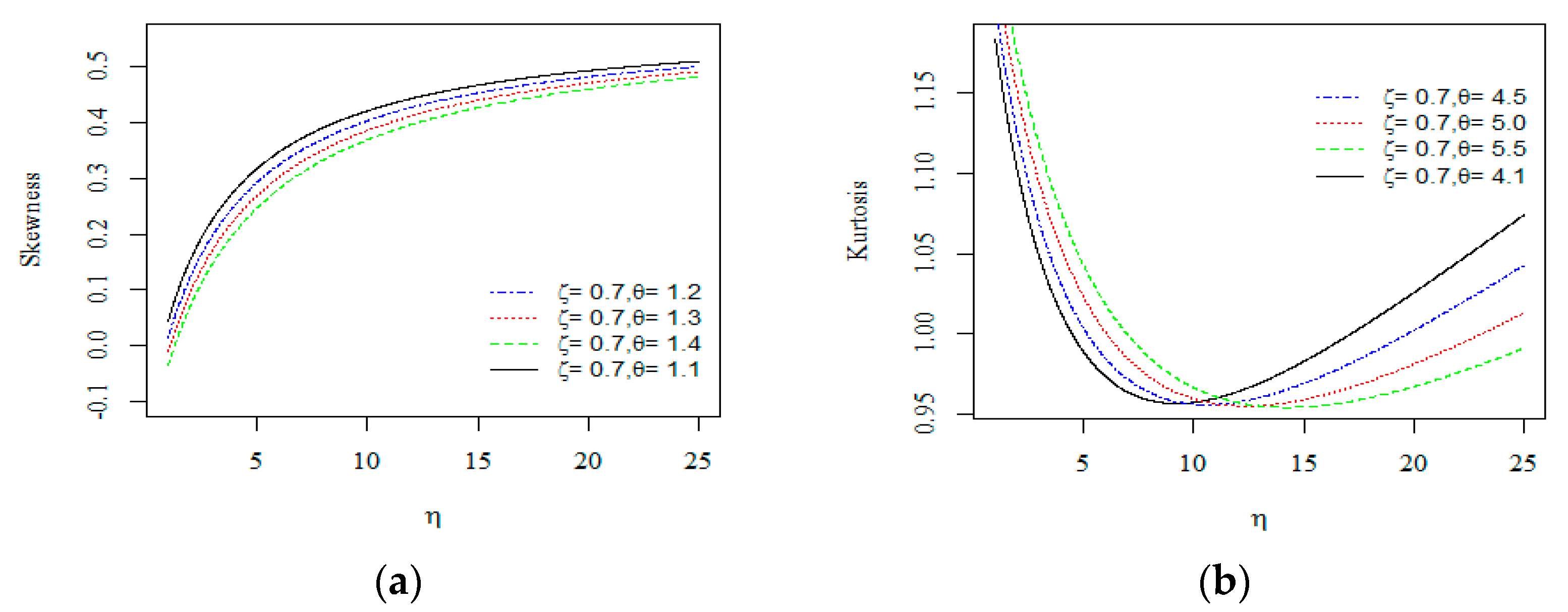
3.5. Quantile Function, Skewness, and Kurtosis

Hyndman and Fan [29] introduced the concept of quantile function (QF). The q-th QF of the E-NPF distribution can be adapted to generate random numbers and is obtained by inverting its CDF (1). The QF is defined by $q=F\left(x_q\right)=P\left(X\le x_q\right), q\in \left(0,1\right).$ Then, the QF of X follows as

$$x_q=\frac{1-{\left(1-q^{\frac{1}{\theta }}\right)}^{\frac{1}{\zeta }}}{1+\eta {\left(1-q^{\frac{1}{\theta }}\right)}^{\frac{1}{\zeta }}} .$$

(14)

To derive the 1st quartile, median, and 3rd quartile of $X$, one may place q = 0.25, 0.5, and 0.75, respectively, in Equation (14).

The Bowley [30] skewness, say $B$, and Moors [31] kurtosis, say $M$, of the E-NPF distribution can be calculated using Equation (14) with the following two formulas:

$$B=\frac{Q_{0.75}+Q_{0.25}-2Q_{0.50}}{Q_{0.75}-Q_{0.25}}$$

and

$$M=\frac{Q_{0.375}-Q_{0.125}-Q_{0.625}+Q_{0.875}}{Q_{0.75}-Q_{0.25}}.$$

These descriptive measures depend on quartiles and octiles and can provide more robust estimates than the traditional measures of skewness and kurtosis. Additionally, $B$ and $M$ are less sensitive to the outliers and work more effectively for the deficient moment distributions. Some possible shapes of the skewness and kurtosis for various choices of $\eta ,\zeta$ and $\theta$ are presented in Figure 3.

3.6. Moments and Associated Measures

Moments have a useful role in distribution theory, to address the significant characteristics of a probability distribution such as mean, variance, skewness, and kurtosis.

Theorem 1.

If$X~$E-NPF($\eta ,\zeta ,\theta$), with$\eta ,\zeta ,\theta >0$, then the r-th ordinary moment (${\mu }_{ r}^{\prime }$) of$X$is given by

$${\mu }_{ r}^{\prime }=\zeta \theta \left(1+\eta \right){\displaystyle \sum }_{i=0}^{\infty }{\displaystyle \sum }_{j=0}^{\infty }{(-1)}^i{\eta }^j\left(\begin{array}{c}\theta -1\\ i\end{array}\right)\left(\begin{array}{c}\alpha \\ j\end{array}\right)B\left(r+j+1,\zeta \left(1+i\right)\right),$$

where B($a,b$) = ${{\displaystyle \int }}_0^1{t}^a{\left(1-t\right)}^{b-1}dt$ is the beta function (BF).

Proof. 

Using Equation (2), ${\mu }_{ r}^{\prime }$ can be written as

$${\mu }_{ r}^{\prime }=\theta \zeta \left(1+\eta \right){{\displaystyle \int }}_0^1\frac{x^r}{{\left(1+\eta x\right)}^2}{\left(\frac{1-x}{1+\eta x}\right)}^{\zeta -1}{\left(1-{\left(\frac{1-x}{1+\eta x}\right)}^{\zeta }\right)}^{\theta -1}dx.$$

After some algebra, we get

$${\mu }_{ r}^{\prime }=\zeta \theta \left(1+\eta \right){\displaystyle \sum }_{i=0}^{\infty }{\displaystyle \sum }_{j=0}^{\infty }{(-1)}^i{\eta }^j\left(\begin{array}{c}\theta -1\\ i\end{array}\right)\left(\begin{array}{c}\alpha \\ j\end{array}\right){{\displaystyle \int }}_0^1{x}^{r+j}{\left(1-x\right)}^{\zeta \left(1+i\right)-1}dx.$$

Simple computations on the last expression lead to the final form of ${\mu }_{ r}^{\prime }$ as follows:

$${\mu }_{ r}^{\prime }=\zeta \theta \left(1+\eta \right){\displaystyle \sum }_{i=0}^{\infty }{\displaystyle \sum }_{j=0}^{\infty }{(-1)}^i{\eta }^j\left(\begin{array}{c}\theta -1\\ i\end{array}\right)\left(\begin{array}{c}\alpha \\ j\end{array}\right)B\left(r+j+1,\zeta \left(1+i\right)\right),$$

(15)

where B($x;a,b$) = ${{\displaystyle \int }}_0^x{t}^{a-1}{\left(1-t\right)}^{b-1}dt$ is the BF and $\alpha =-\zeta \left(1+i\right)-1.$ □

The moment formula (15) is supportive in the development of some useful statistical measures. For instance, the mean of $X$ follows with $r=1$ in Equation (15). The 2nd, 3rd, 4th, and higher-order moments of $X$ are formulated by replacing r = 2, 3, and 4 in Equation (15), respectively. Additionally, the Fisher index (F.I. = ($Var\left(X\right)/E\left(X\right)$)) plays a significant role in discussing the variability in $X$. The negative moment of $X$ is simply derived through substituting r by –w in (15). Moreover, one can calculate the skewness (${\tau }_1={\mu }_3^2/{\mu }_2^3$) and kurtosis (${\tau }_2={\mu }_4/{\mu }_2^2$) of $X$ by integrating Equation (15). Well-established relationships between the central moments $\left({\mu }_s\right)$ and cumulants ($K_s$) of $X$ may easily be defined through ${\mu }_{ r}^{\prime }$. The moment generating (MG) function of $X$, $M_X\left(t\right)$, is defined by

$$M_X\left(t\right)={\displaystyle \sum }_{r=0}^{\infty } \frac{t^r}{r!} {\mu }_r^{\prime }.$$

The MG function of $X$ follows as

$$M_X\left(t\right)=2\beta \gamma \zeta \theta \left(1+\eta \right){\displaystyle \sum }_{r=0}^{\infty }\frac{t^r}{r!}{\displaystyle \sum }_{i=0}^{\infty }{\displaystyle \sum }_{j=0}^{\infty }{(-1)}^i{\eta }^j\left(\begin{array}{c}\theta -1\\ i\end{array}\right)\left(\begin{array}{c}\alpha \\ j\end{array}\right)B\left(r+j+1,\zeta \left(1+i\right)\right).$$

Table 2. Some numerical results of moments, variance (${\epsilon }^2$), skewness (${\tau }_1$), and kurtosis (${\tau }_2$).

${{\mu }^{\prime }}_s$	S-I	S-II	S-III	S-IV	S-V
${{\mu }^{\prime }}_1$	0.2874	0.3528	0.0599	0.4500	0.3581
${{\mu }^{\prime }}_2$	0.1582	0.1794	0.0107	0.2543	0.1714
${{\mu }^{\prime }}_3$	0.1064	0.1101	0.0031	0.1645	0.0990
${{\mu }^{\prime }}_4$	0.0790	0.0753	0.0011	0.1162	0.0647
${\epsilon }^2$	0.0701	0.0342	0.0013	0.0010	0.0094
${\tau }_1$	0.0203	0.0621	8.3037	0.0694	0.3347
${\tau }_2$	0.5630	0.2697	2.7600	−0.1506	−0.1713

displays some numerical results of the first four moments ${{\mu }^{\prime }}_1,{{\mu }^{\prime }}_2,{{\mu }^{\prime }}_3,{{\mu }^{\prime }}_4$, variance ${\epsilon }^2$, ${\tau }_1$, and ${\tau }_2$ for some choices of $\eta ,\zeta$ and $\theta$. The results are presented for S-I($\eta =0.1, \zeta =1.2,\theta =0.5$), S-II($\eta =1.1, \zeta =1.5,\theta =1.5$), S-III($\eta =2.1, \zeta =3.5,\theta =0.5$), S-IV($\eta =1.1, \zeta =1.5,\theta =2.5$), and S-V($\eta =4.1, \zeta =1.5,\theta =3.9$). The results indicate that the moments and variance decrease gradually, though skewness falls between 0 and 1, and kurtosis might be negative as per the different combinations of the parameters.

3.7. Incomplete Moments

Incomplete moments (IM) are categorized into the lower IM (LIM) and the upper IM (UIM).

The r-th LIM is defined as ${\Phi }_r\left(t\right)={{\displaystyle \int }}_0^t{x}^{r}f\left(x\right)dx.$

The LIM of $X$ has the form

$${\Phi }_r\left(t\right)=\zeta \theta \left(1+\eta \right){\displaystyle \sum }_{i=0}^{\infty }{\displaystyle \sum }_{j=0}^{\infty }{(-1)}^i{\eta }^j\left(\begin{array}{c}\theta -1\\ i\end{array}\right)\left(\begin{array}{c}\alpha \\ j\end{array}\right)B_t\left(r+j+1,\zeta \left(1+i\right)\right),$$

(16)

where B($x;a,b$) = ${{\displaystyle \int }}_0^x{t}^{a-1}{\left(1-t\right)}^{b-1}dt$ is the BF and $\alpha =-\zeta \left(1+i\right)-1 .$

The conditional survivor/residual life function is the probability that the life of a component, say x, will survive in an additional interval at t.

It is given by

$$R\left(t|x\right)=P\left(X>x+t|X>t\right)=\frac{R\left(X>x+t\right)}{P\left(X>t\right)}=\frac{R\left(x+t\right)}{S\left(t\right)}.$$

The residual life function of X has the form

$$S_{R\left(t\right)}\left(t|x\right)=\frac{1-{\left(1-{\left(\frac{1-\left(x+t\right)}{1+\eta \left(x+t\right)}\right)}^{\zeta }\right)}^{\theta }}{1-{\left(1-{\left(\frac{1-t}{1+\eta t}\right)}^{\zeta }\right)}^{\theta }}.$$

(17)

Furthermore, the reverse residual life is obtained by $S_{\overline{R}\left(t\right)}\left(t|x\right)=\frac{S\left(x-t\right)}{S\left(t\right)}.$ It is derived for $X$ by the formula

$$S_{\overline{R}\left(t\right)}\left(t|x\right)=\frac{1-{\left(1-{\left(\frac{1-\left(x-t\right)}{1+\eta \left(x-t\right)}\right)}^{\zeta }\right)}^{\theta }}{1-{\left(1-{\left(\frac{1-t}{1+\eta t}\right)}^{\zeta }\right)}^{\theta }}.$$

(18)

3.8. Entropy

In general, entropy is defined as the system’s disorderedness, uncertainty, or a measure of entanglement.

The Rényi [32] entropy is given as follows:

$$H_{\varphi }\left(X\right)=\frac{1}{1-\varphi }\log \underset{0}{\overset{1}{{\displaystyle \int }}}{f}^{\varphi }\left(x\right)dx , \varphi >0 \mathrm{and} \varphi \ne 1.$$

(19)

First, using Equation (2), we get

$$f^{\varphi }\left(x;\eta ,\zeta ,\theta \right)={\left(\frac{\theta \zeta \left(1+\eta \right)}{{\left(1+\eta x\right)}^2}\right)}^{\varphi }{\left(\frac{1-x}{1+\eta x}\right)}^{\varphi \left(\zeta -1\right)}{\left(1-{\left(\frac{1-x}{1+\eta x}\right)}^{\zeta }\right)}^{\varphi \left(\theta -1\right)}{}^{ }.$$

By applying the binomial expansion to the last expression, Equation (19) takes the form

$$\begin{gathered} H_{\varphi }\left(X\right)=\frac{1}{1-\varphi }\log {\left({\left(\theta \zeta \left(1+\eta \right)\right)}^{\varphi }{\displaystyle \sum }_{i=0}^{\infty }{\displaystyle \sum }_{j=0}^{\infty }{(-1)}^i{\eta }^j\left(\begin{array}{c}\left(\theta -1\right)\varphi \\ i\end{array}\right)\left(\begin{array}{c}-\varphi \left(\zeta +1\right)-\zeta i\\ j\end{array}\right)\right)}^{ } \\ \times \underset{0}{\overset{1}{{\displaystyle \int }}}{x}^j{\left(1-x\right)}^{\varphi \left(\zeta -1\right)+\zeta i}dx, \end{gathered}$$

Hence, the simplified form of $H_{\varphi }\left(X\right)$ follows as

$$H_{\varphi }\left(X\right)=\frac{1}{1-\varphi }\log \left({\displaystyle \sum }_{i=0}^{\infty }{\displaystyle \sum }_{j=0}^{\infty }\frac{S_{i,j}\left(\eta ,\varphi ,\zeta ,\theta \right)}{{\left[\theta \zeta \left(1+\eta \right)\right]}^{-\varphi }}B\left(j+1, \varphi \left(\zeta -1\right)+\zeta i+1\right)\right),$$

(20)

where $S_{i,j}\left(\eta ,\varphi ,\zeta ,\theta \right)={(-1)}^i{\eta }^j\left(\begin{array}{c}\left(\theta -1\right)\varphi \\ i\end{array}\right)\left(\begin{array}{c}-\varphi \left(\zeta +1\right)-\zeta i\\ j\end{array}\right).$

3.9. Stress–Strength Reliability

Let X₁ and X₂ be defined to discuss the strength and stress of a component, respectively. The reliability, say R, of $X$ is defined (for $X_2<X_1$) by $R=P\left(X_2<X_1\right).$

Theorem 2.

Let$X_1~$E-NPF($\eta ,\zeta ,{\theta }_1$) and$X_2~$E-NPF($\eta ,\zeta ,{\theta }_2$) be independent random variables, then the reliability R reduces to

$$R=\frac{{\theta }_1}{{\theta }_1+{\theta }_2} .$$

Proof. 

The reliability R is given by

$$R=P\left(X_2<X_1\right)={\displaystyle \int f_1}\left(x\right)F_2\left(x\right)dx.$$

Hence, R reduces to

$$R={\displaystyle \int }\left(\frac{d}{dx}{\left(1-{\left(\frac{1-x}{1+\eta x}\right)}^{\zeta }\right)}^{{\theta }_1}\right){\left(1-{\left(\frac{1-x}{1+\eta x}\right)}^{\zeta }\right)}^{{\theta }_2}dx.$$

(21)

$$\mathrm{Let}{\left(1-{\left(\frac{1-x}{1+\eta x}\right)}^{\zeta }\right)}^{{\theta }_1}=z \Rightarrow {\left(1-{\left(\frac{1-x}{1+\eta x}\right)}^{\zeta }\right)}^{{\theta }_2}=z^{\frac{{\theta }_2}{{\theta }_1}}.$$

On simplification, Equation (21) takes the form

$$R={\displaystyle \int }{z}^{\frac{{\theta }_2}{{\theta }_1}} dz.$$

After simple computations, R can be expressed in terms of ${\theta }_1$ and ${\theta }_2$ as

$$R=\frac{{\theta }_1}{{\theta }_1+{\theta }_2} \mathrm{for} {\theta }_1,{\theta }_2>0.$$

The last expression illustrates that the reliability R of the E-NPF distribution is an increasing function of ${\theta }_1$ and a decreasing function of ${\theta }_2$. □

3.10. Stochastic Ordering

Over the past 40 years, the concept of stochastic ordering has engaged scientists and practitioners and is quite useful in economics, reliability theory, queuing theory, insurance, and ecology, among other fields of science.

Let X₁ and X₂ be the two continuous, nonnegative, and univariate random variables, with Q₁(X) and Q₂(X) being the CDFs with corresponding PDFs q₁(x) and q₂(x), respectively. The random variable X₁ is smaller than X₂ under the following constraints:

(i)

stochastic order (st) (denoted by X₁ ${\le }_{st}$ X₂) if Q₁(X) $\le$ Q₂(X) $\forall$ x;

(ii)

reversed hazard rate (rhr) order (denoted by X₁ ${\le }_{rhr}$ X₂) if Q₁(X)/Q₂(X) is decreasing for x $\ge$ 0;

(iii)

likelihood ratio (lkr) order (denoted by X₁ ${\le }_{lkr}$ X₂) if Q₁(x)/Q₂(x) is decreasing for x $\ge$ 0;

(iv)

hazard rate (hr) order (denoted by X₁ ${\le }_{hr}$ X₂) if Q₁(X)/Q₂(X) is decreasing for x $\ge$ 0.

The four stochastic orders are connected to each other based on the following implications [33].

$$X_1{\le }_{rhr}{X}_2\Leftarrow X_1{\le }_{lkr}{X}_2\Rightarrow X_1{\le }_{hr}{X}_2\Rightarrow X_1{\le }_{st}{X}_2.$$

Theorem 3.

Let X₁$~$E-NPF($\eta ,\zeta ,{\theta }_1$) and X₂$~$E-NPF($\eta ,\zeta ,{\theta }_2$), if ${\theta }_1<$ ${\theta }_2$, then X₁ ${\le }_{lkr}$X₂ and hence X₁ ${\le }_{rhr}$ X₂ $\Rightarrow$ X₁ ${\le }_{hr}$ X₂ $\Rightarrow$ and X₁ ${\le }_{st}$ X₂.

Proof. 

Using Equation (2), we have

$$f_1\left(x;\eta ,\zeta ,{\theta }_1\right)=\frac{{\theta }_1\zeta \left(1+\eta \right)}{{\left(1+\eta x\right)}^2}{\left(\frac{1-x}{1+\eta x}\right)}^{\zeta -1}{\left(1-{\left(\frac{1-x}{1+\eta x}\right)}^{\zeta }\right)}^{{\theta }_1-1}$$

(22)

and

$$f_2\left(x;\eta ,\zeta ,{\theta }_2\right)=\frac{{\theta }_2\zeta \left(1+\eta \right)}{{\left(1+\eta x\right)}^2}{\left(\frac{1-x}{1+\eta x}\right)}^{\zeta -1}{\left(1-{\left(\frac{1-x}{1+\eta x}\right)}^{\zeta }\right)}^{{\theta }_2-1}.$$

(23)

Hence, we can write

$$\frac{f_1\left(x;\eta ,\zeta ,{\theta }_1\right)}{f_2\left(x;\eta ,\zeta ,{\theta }_2\right)}=\frac{{\theta }_1}{{\theta }_2}{\left(1-{\left(\frac{1-x}{1+\eta x}\right)}^{\zeta }\right)}^{{\theta }_1-{\theta }_2}.$$

By taking derivative w.r.t x on both sides, we get

$$\frac{d}{dx}\left(\frac{f_1\left(x;\eta ,\zeta ,{\theta }_1\right)}{f_2\left(x;\eta ,\zeta ,{\theta }_2\right)}\right)=\frac{{\theta }_1}{{\theta }_2}\left({\theta }_1-{\theta }_2\right){\left(1-{\left(\frac{1-x}{1+\eta x}\right)}^{\zeta }\right)}^{{\theta }_1-{\theta }_2-1}\left(\frac{\zeta \left(1+\eta \right){\left(1-x\right)}^{\zeta -1}}{{\left(1+\eta x\right)}^{\zeta +1}}\right).$$

Then,

$$\frac{d}{dx}\left(\frac{f_1\left(x;\eta ,\zeta ,{\theta }_1\right)}{f_2\left(x;\eta ,\zeta ,{\theta }_2\right)}\right)<0\Rightarrow \frac{f_1\left(x;\eta ,\zeta ,{\theta }_1\right)}{f_2\left(x;\eta ,\zeta ,{\theta }_2\right)}$$

is a decreasing function for all ${\theta }_1<$ ${\theta }_2$.

Hence, X₁ ${\le }_{lkr}$ X₂ for ${\theta }_1<$ ${\theta }_2$. □

3.11. Order Statistics

Order statistics (OS) and their moments are considered noteworthy measures in quality control, reliability analysis, and life testing. Let $X_1, X_2, \dots ,X_n$ be a random sample of size n that follows the E-NPF distribution and $X_{\left(1:n\right)}<X_{\left(2:n\right)}<X_{\left(3:n\right)}<\dots <X_{\left(n:n\right)}$ be the corresponding OS.

The PDF of $X_{\left(i:n\right)}$ is

$$f_{\left(i:n\right)}\left(x\right)=\frac{1}{B\left(i, n-i+1\right)} {\left(F\left(x\right)\right)}^{i-1} {\left(1-F\left(x\right)\right)}^{n-i} f\left(x\right), i=1,2,3,\dots ,n.$$

By replacing (1) and (2) in the above equation, the PDF of $X_{\left(i\right)}$ takes the form

$$\begin{gathered} f_{\left(i:n\right)}\left(x\right)=\frac{1}{B\left(i, n-i+1\right)}\frac{\theta \zeta \left(1+\eta \right)}{{\left(1+\eta x\right)}^2}{\left({\left(1-{\left(\frac{1-x}{1+\eta x}\right)}^{\zeta }\right)}^{\theta }\right)}^{i-1}{\left(\frac{1-x}{1+\eta x}\right)}^{\zeta -1} \\ \times {\left(1-{\left(\frac{1-x}{1+\eta x}\right)}^{\zeta }\right)}^{\theta -1}{\left(1-{\left(1-{\left(\frac{1-x}{1+\eta x}\right)}^{\zeta }\right)}^{\theta }\right)}^{n-i}. \end{gathered}$$

The above equation is adopted to compute the w-th moment OS of the E-NPF distribution. Furthermore, the minimum and maximum OS of $X$ follow directly from the above equation with $i=1,2$, respectively. The w-th moment OS, $E\left(X_{OS}^w\right)$, of $X$ follows as

$$\begin{gathered} E\left(X_{OS}^w\right)=\frac{\zeta \theta \left(1+\eta \right)}{B\left(i, n-i+1\right)!}{\displaystyle \sum }_{j=0}^{\infty }{\displaystyle \sum }_{k=0}^{\infty }{\displaystyle \sum }_{l=0}^{\infty }{(-1)}^{j+k}{\eta }^j\left(\begin{array}{c}\eta -i\\ j\end{array}\right)\left(\begin{array}{c}\theta \left(i+j\right)-1\\ k\end{array}\right) \\ \times \left(\begin{array}{c}-\left(\zeta k+\zeta +1\right)\\ l\end{array}\right) B\left(r+l-1,\zeta k+\zeta \right). \end{gathered}$$

The CDF of $X_{\left(i:n\right)}$ is defined (for $i=1,2,3,\dots ,n$) by

$$F_{\left(i:n\right)}\left(x\right)={\displaystyle \sum }_{r=i}^n\left(\begin{array}{c}n\\ r\end{array}\right){\left(F\left(x\right)\right)}^r {\left(1-F\left(x\right)\right)}^{n-r} .$$

For the E-NPF model, the CDF of $X_{\left(i:n\right)}$ reduces to

$$F_{\left(i:n\right)}\left(x\right)={\displaystyle \sum }_{r=i}^n\left(\begin{array}{c}n\\ r\end{array}\right){\left({\left(1-{\left(\frac{1-x}{1+\eta x}\right)}^{\zeta }\right)}^{\theta }\right)}^r{\left(1-{\left(1-{\left(\frac{1-x}{1+\eta x}\right)}^{\zeta }\right)}^{\theta }\right)}^{n-r}.$$

4. Estimation of the E-NPF Distribution

4.1. Estimation under Complete Samples

In this section, we estimate the E-NPF parameters $\eta$, $\zeta ,$and $\theta$ using eight frequentist approaches under complete samples.

4.1.1. Maximum Likelihood Estimation under Complete Samples

In this section, we estimate the parameters of the E-NPF distribution using the maximum likelihood (ML) method. Let $X_1,X_2, \dots ,X_n$ be a random sample of size n from the E-NPF distribution, then the likelihood function of $X$, $L \left(\Theta \right)$, takes the form

$$L \left(\Theta \right)={\theta }^n {\zeta }^n {\left(1+\eta \right)}^n {{\displaystyle \prod }}_{i=1}^{n }\frac{{\left(1-x_i\right)}^{\zeta -1}}{{\left(1+\eta x_i\right)}^{\zeta +1}} {\left(1-{\left(\frac{1-x_i}{1+\eta x_i}\right)}^{\zeta }\right)}^{\theta -1}.$$

The log-likelihood function, $\ell \left(\Theta \right)=\log L\left(\Theta \right)$, of $X$ is

$$\begin{gathered} \ell \left(\Theta \right)=n\left(\log \theta +\log \zeta +\log \left(1+\eta \right)\right)+\left(\zeta -1\right){\displaystyle \sum }_{i=1}^n\log \left(1-x_i\right) \\ -\left(\zeta +1\right){\displaystyle \sum }_{i=1}^n\log \left(1+\eta x_i\right)+\left(\theta -1\right){\displaystyle \sum }_{i=1}^n\log \left(1-{\left(\frac{1-x_i}{1+\eta x_i}\right)}^{\zeta }\right). \end{gathered}$$

(24)

By taking partial derivatives of Equation (24), we get

$$\begin{gathered} \frac{\partial \ell \left(\Theta \right)}{\partial \eta }=\frac{n}{1+\eta }-\left(\zeta +1\right){\displaystyle \sum }_{i=1}^n\left(\frac{x_i}{1+\eta x_i }\right)+\zeta \left(\theta -1\right){\displaystyle \sum }_{i=1}^n\frac{x_i{\left(1-x_i\right)}^{\zeta }{\left(1+\eta x_i\right)}^{-\zeta -1}}{1-{\left(\frac{1-x_i}{1+\eta x_i}\right)}^{\zeta }}, \\ \frac{\partial \ell \left(\Theta \right)}{\partial \zeta }=\frac{n}{\zeta }+{\displaystyle \sum }_{i=1}^n\log \left(\frac{1-x_i}{1+\eta x_i }\right)-\left(\theta -1\right){\displaystyle \sum }_{i=1}^n\frac{{\left(\frac{1-x_i}{1+\eta x_i}\right)}^{\zeta }\log \left(\frac{1-x_i}{1+\eta x_i}\right)}{\left(1-{\left(\frac{1-x_i}{1+\eta x_i}\right)}^{\zeta }\right)} \end{gathered}$$

and

$$\frac{\partial \ell \left(\Theta \right)}{\partial \theta }=\frac{n}{\theta }+{\displaystyle \sum }_{i=1}^n\log \left(1-{\left(\frac{1-x_i}{1+\eta x_i }\right)}^{\zeta }\right).$$

The ML estimators (MLE) ${\widehat{\eta }}_{MLE}$, ${\widehat{\zeta }}_{MLE}$ and ${\widehat{\theta }}_{MLE}$ of the E-NPF distribution can be obtained by maximizing Equation (24) or by solving the above equations simultaneously. These equations cannot provide analytical solutions for the MLEs and the optimum values of $\eta ,\zeta ,$ and $\theta$. Consequently, the Newton–Raphson-type algorithm is an appropriate way in the support of the MLE. This can be done by using different programs, namely $R$ (optim function), Mathematica, or SAS (PROC NLMIXED), or by solving the nonlinear likelihood equations determined by differentiating $\ell \left(\Theta \right)$.

4.1.2. Ordinary and Weighted Least-Squares Estimators

Let $x_{\left(1\right)},x_{\left(2\right)},\cdots ,x_{\left(n\right)}$ be the OS of the random sample of size $n$ from $F_{\mathrm{E}-\mathrm{NPF}}\left(x;\eta ,\zeta ,\theta \right)$ in (1). The ordinary least-squares estimators (OLSE), ${\widehat{\eta }}_{LSE}$, ${\widehat{\zeta }}_{LSE}$ and ${\widehat{\theta }}_{LSE}$, can be obtained by minimizing

$$V\left(\eta ,\zeta ,\theta \right)={\displaystyle \sum }_{i=1}^n{\left[F_{\mathrm{E}-\mathrm{NPF}}\left(x_{\left(i\right)}|\eta ,\zeta ,\theta \right)-\frac{i}{n+1}\right]}^2,$$

with respect to $\alpha$, $\mu$, and $\sigma$. Or equivalently, the OLSE follow by solving the nonlinear equations

$${\displaystyle \sum }_{i=1}^n\left[F_{\mathrm{E}-\mathrm{NPF}}\left(x_{\left(i\right)}|\eta ,\zeta ,\theta \right)-\frac{i}{n+1}\right]{\mathsf{\Delta }}_s\left(x_{\left(i\right)}|\eta ,\zeta ,\theta \right)=0,s=1,2,3,$$

where

$$\begin{gathered} {\mathsf{\Delta }}_1\left(x_{\left(i\right)}|\eta ,\zeta ,\theta \right)=\frac{\partial }{\partial \eta }{F}_{\mathrm{E}-\mathrm{NPF}}\left(x_{\left(i\right)}|\eta ,\zeta ,\theta \right), \\ {\mathsf{\Delta }}_2\left(x_{\left(i\right)}|\eta ,\zeta ,\theta \right)=\frac{\partial }{\partial \zeta }{F}_{\mathrm{E}-\mathrm{NPF}}\left(x_{\left(i\right)}|\eta ,\zeta ,\theta \right)\mathrm{and} \end{gathered}$$

$${\mathsf{\Delta }}_3\left(x_{\left(i\right)}|\eta ,\zeta ,\theta \right)=\frac{\partial }{\partial \theta }{F}_{\mathrm{E}-\mathrm{NPF}}\left(x_{\left(i\right)}|\eta ,\zeta ,\theta \right).$$

$$\begin{gathered} {\mathsf{\Delta }}_1\left(x_{\left(i\right)}|\eta ,\zeta ,\theta \right)=\frac{\partial }{\partial \eta }{F}_{\mathrm{E}-\mathrm{NPF}}\left(x_{\left(i\right)}|\eta ,\zeta ,\theta \right),{\mathsf{\Delta }}_2\left(x_{\left(i\right)}|\eta ,\zeta ,\theta \right)=\frac{\partial }{\partial \zeta }{F}_{\mathrm{E}-\mathrm{NPF}}\left(x_{\left(i\right)}|\eta ,\zeta ,\theta \right)\mathrm{and} \\ {\mathsf{\Delta }}_3\left(x_{\left(i\right)}|\eta ,\zeta ,\theta \right)=\frac{\partial }{\partial \theta }{F}_{\mathrm{E}-\mathrm{NPF}}\left(x_{\left(i\right)}|\eta ,\zeta ,\theta \right). \end{gathered}$$

(25)

Note that the solution of ${\mathsf{\Delta }}_s$ for $s=1,2,3$ can be obtained numerically.

The weighted least-squares estimators (WLSE), ${\widehat{\eta }}_{WLSE}$, ${\widehat{\zeta }}_{WLSE}$, and ${\widehat{\theta }}_{WLSE}$, can be obtained by minimizing the following equation:

$$W\left(\eta ,\zeta ,\theta \right)={\displaystyle \sum }_{i=1}^n\frac{{\left(n+1\right)}^2\left(n+2\right)}{i\left(n-i+1\right)}{\left[F_{\mathrm{E}-\mathrm{NPF}}\left(x_{\left(i\right)}|\eta ,\zeta ,\theta \right)-\frac{i}{n+1}\right]}^2.$$

Furthermore, the WLSE can also be derived by solving the nonlinear equations

$${\displaystyle \sum }_{i=1}^n\frac{{\left(n+1\right)}^2\left(n+2\right)}{i\left(n-i+1\right)}\left[F_{\mathrm{E}-\mathrm{NPF}}\left(x_{\left(i\right)}|\eta ,\zeta ,\theta \right)-\frac{i}{n+1}\right]{\mathsf{\Delta }}_s\left(x_{\left(i\right)}|\eta ,\zeta ,\theta \right)=0,s=1,2,3$$

where ${\mathsf{\Delta }}_1\left(\cdot |\eta ,\zeta ,\theta \right)$, ${\mathsf{\Delta }}_2\left(\cdot |\eta ,\zeta ,\theta \right),$ and ${\mathsf{\Delta }}_3\left(\cdot |\eta ,\zeta ,\theta \right)$ are provided in (25).

4.1.3. Maximum Product of Spacing

The maximum product of spacing (MPS) method, as an approximation to the Kullback–Leibler information measure, is a good alternative to the MLE method.

Let $D_i\left(\eta ,\zeta ,\theta \right)=F_{\mathrm{E}-\mathrm{NPF}}\left(x_{\left(i\right)}|\eta ,\zeta ,\theta \right)-F_{\mathrm{E}-\mathrm{NPF}}\left(x_{\left(i-1\right)}|\eta ,\zeta ,\theta \right)$, for $i=1,2,\dots ,n+1,$ be the uniform spacing of a random sample from the E-NPF distribution, where $F_{\mathrm{E}-\mathrm{NPF}}\left(x_{\left(0\right)}|\eta ,\zeta ,\theta \right)=0$, $F_{\mathrm{E}-\mathrm{NPF}}\left(x_{\left(n+1\right)}|\eta ,\zeta ,\theta \right)=1$, and ${\displaystyle \sum }_{i=1}^{n+1}{D}_i\left(\eta ,\zeta ,\theta \right)=1.$ The MPS estimators (MPSE) for ${\widehat{\eta }}_{MPSE}$, ${\widehat{\zeta }}_{MPSE}$, and ${\widehat{\theta }}_{MPSE}$ can be obtained by maximizing the geometric mean of the spacing

$$F\left(\eta ,\zeta ,\theta \right)={\left[{\displaystyle \prod }_{i=1}^{n+1}{D}_i\left(\eta ,\zeta ,\theta \right)\right]}^{\frac{1}{n+1}}$$

with respect to $\eta ,\zeta$, and $\theta$, or, equivalently, by maximizing the logarithm of the geometric mean of sample spacings.

$$H\left(\eta ,\zeta ,\theta \right)=\frac{1}{n+1}{\displaystyle \sum }_{i=1}^{n+1}\log \left(D_i\left(\eta ,\zeta ,\theta \right)\right).$$

The MPSE of the E-NPF parameters can be obtained by solving the nonlinear equations defined by

$$\frac{1}{n+1}{\displaystyle \sum }_{i=1}^{n+1}\frac{1}{D_i\left(\eta ,\zeta ,\theta \right)}\left[{\mathsf{\Delta }}_s\left(x_{\left(i\right)}|\eta ,\zeta ,\theta \right)-{\mathsf{\Delta }}_s\left(x_{\left(i-1\right)}|\eta ,\zeta ,\theta \right)\right]=0,s=1,2,3,$$

where ${\mathsf{\Delta }}_1\left(\cdot |\eta ,\zeta ,\theta \right)$, ${\mathsf{\Delta }}_2\left(\cdot |\eta ,\zeta ,\theta \right),$ and ${\mathsf{\Delta }}_3\left(\cdot |\eta ,\zeta ,\theta \right)$ are provided in (25).

4.1.4. The Cramér–von Mises Estimators

The Cramér–von Mises estimators (CVME) as a type of minimum distance (MD) estimator have less bias than the other MD estimators. The CVME are obtained based on the difference between the estimates of the CDF and the empirical distribution function. The CVME of the E-NPF parameters, ${\widehat{\eta }}_{CVME}$, ${\widehat{\zeta }}_{CVME}$, and ${\widehat{\theta }}_{CVME}$, can be obtained by minimizing

$$C\left(\eta ,\zeta ,\theta \right)=\frac{1}{12n}+{\displaystyle \sum }_{i=1}^n{\left[F_{\mathrm{E}-\mathrm{NPF}}\left(x_{\left(i\right)}|\eta ,\zeta ,\theta \right)-\frac{2i-1}{2n}\right]}^2,$$

with respect to $\eta , \zeta$, and $\theta$. Furthermore, the CVME follow by solving the nonlinear equations

$${\displaystyle \sum }_{i=1}^n\left[F_{\mathrm{E}-\mathrm{NPF}}\left(x_{\left(i\right)}|\eta ,\zeta ,\theta \right)-\frac{2i-1}{2n}\right]{\mathsf{\Delta }}_s\left(x_{\left(i\right)}|\eta ,\zeta ,\theta \right)=0,s=1,2,3,$$

where ${\mathsf{\Delta }}_1\left(\cdot |\eta ,\zeta ,\theta \right)$, ${\mathsf{\Delta }}_2\left(\cdot |\eta ,\zeta ,\theta \right)$, and ${\mathsf{\Delta }}_3\left(\cdot |\eta ,\zeta ,\theta \right)$ are provided in (25).

4.1.5. The Anderson–Darling and Right-Tail Anderson–Darling Estimators

The Anderson–Darling (AD) statistic or AD estimator is another type of minimum distance estimator. The AD estimators (ADE) of the E-NPF parameters, ${\widehat{\eta }}_{ADE}$, ${\widehat{\zeta }}_{ADE}$, and ${\widehat{\theta }}_{ADE}$, can be obtained by minimizing

$$A\left(\eta ,\zeta ,\theta \right)=-n-\frac{1}{n}{\displaystyle \sum }_{i=1}^n\left(2i-1\right)\left[\log \left(F_{\mathrm{E}-\mathrm{NPF}}\left(x_{\left(i\right)}|\eta ,\zeta ,\theta \right)\right)+\log \left(S_{\mathrm{E}-\mathrm{NPF}}\left(x_{\left(i\right)}|\eta ,\zeta ,\theta \right)\right)\right],$$

with respect to $\eta$, $\zeta$, and $\theta$. These ADE can also be obtained by solving the nonlinear equations

$${\displaystyle \sum }_{i=1}^n\left(2i-1\right)\left[\frac{{\mathsf{\Delta }}_s\left(x_{\left(i\right)}|\eta ,\zeta ,\theta \right)}{F_{\mathrm{E}-\mathrm{NPF}}\left(x_{\left(i\right)}|\eta ,\zeta ,\theta \right)}-\frac{{\mathsf{\Delta }}_j\left(x_{\left(n+1-i\right)}|\eta ,\zeta ,\theta \right)}{S_{\mathrm{E}-\mathrm{NPF}}\left(x_{\left(n+1-i\right)}|\eta ,\zeta ,\theta \right)}\right]=0,s=1,2,3.$$

The right-tail AD estimators (RADE) of the E-NPF parameters, ${\widehat{\eta }}_{RADE}$, ${\widehat{\zeta }}_{RADE}$, and ${\widehat{\theta }}_{RADE}$, can be obtained by minimizing

$$\begin{gathered} R\left(\eta ,\zeta ,\theta \right)=\frac{n}{2}-2{\displaystyle \sum }_{i=1}^n{F}_{\mathrm{E}-\mathrm{NPF}}\left(x_{i:n}|\eta ,\zeta ,\theta \right) \\ -\frac{1}{n}{\displaystyle \sum }_{i=1}^n\left(2i-1\right)\log \left(S_{\mathrm{E}-\mathrm{NPF}}\left(x_{n+1-i:n}|\eta ,\zeta ,\theta \right)\right), \end{gathered}$$

with respect to $\eta ,\zeta$, and $\theta$. The RADE can also be obtained by solving the nonlinear equations

$$-2{\displaystyle \sum }_{i=1}^n{\mathsf{\Delta }}_s\left(x_{i:n}|\eta ,\zeta ,\theta \right)+\frac{1}{n}{\displaystyle \sum }_{i=1}^n\left(2i-1\right)\frac{{\mathsf{\Delta }}_s\left(x_{\left(n+1-i:m\right)}|\eta ,\zeta ,\theta \right)}{S_{\mathrm{E}-\mathrm{NPF}}\left(x_{\left(n+1-i:m\right)}|\eta ,\zeta ,\theta \right)}=0,s=1,2,3.$$

where ${\mathsf{\Delta }}_1\left(\cdot |\eta ,\zeta ,\theta \right)$, ${\mathsf{\Delta }}_2\left(\cdot |\eta ,\zeta ,\theta \right),$ and ${\mathsf{\Delta }}_3\left(\cdot |\eta ,\zeta ,\theta \right)$ are provided in (25).

4.1.6. Method of Percentile Estimation

Let $q_i=i/\left(n+1\right)$ be an unbiased estimator of $F_{\mathrm{E}-\mathrm{NPF}}\left(x_{\left(i\right)}|\eta ,\zeta ,\theta \right)$. Then, the percentile estimators (PCE) of the parameters of the E-NPF distribution are obtained by minimizing the following function:

$$P\left(\eta ,\zeta ,\theta \right)={\displaystyle \sum }_{i=1}^n{\left(x_{\left(i\right)}-x_{q_i}\right)}^2,$$

with respect to $\eta ,\zeta$, and $\theta$, where $x_q$ is the QF of the E-NPF distribution defined in (14).

4.2. Estimation under Type II Censored Samples

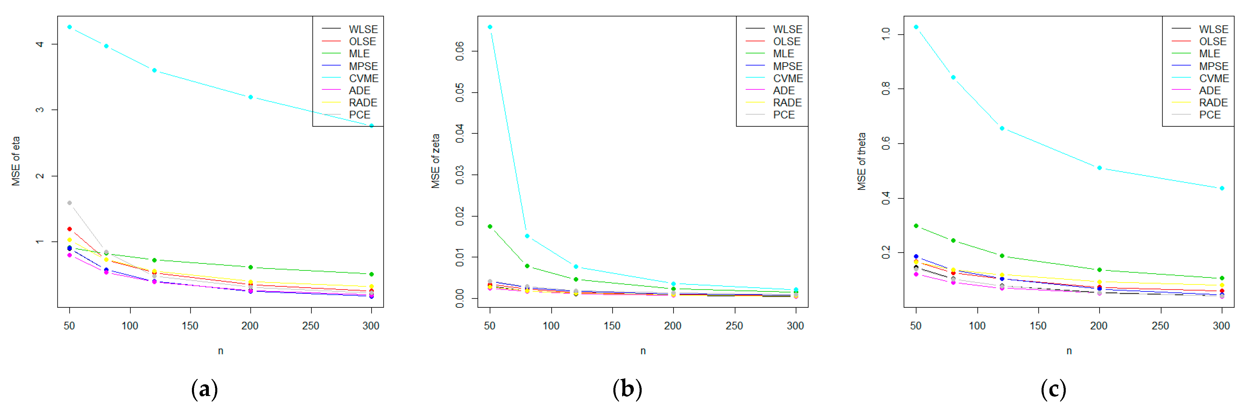
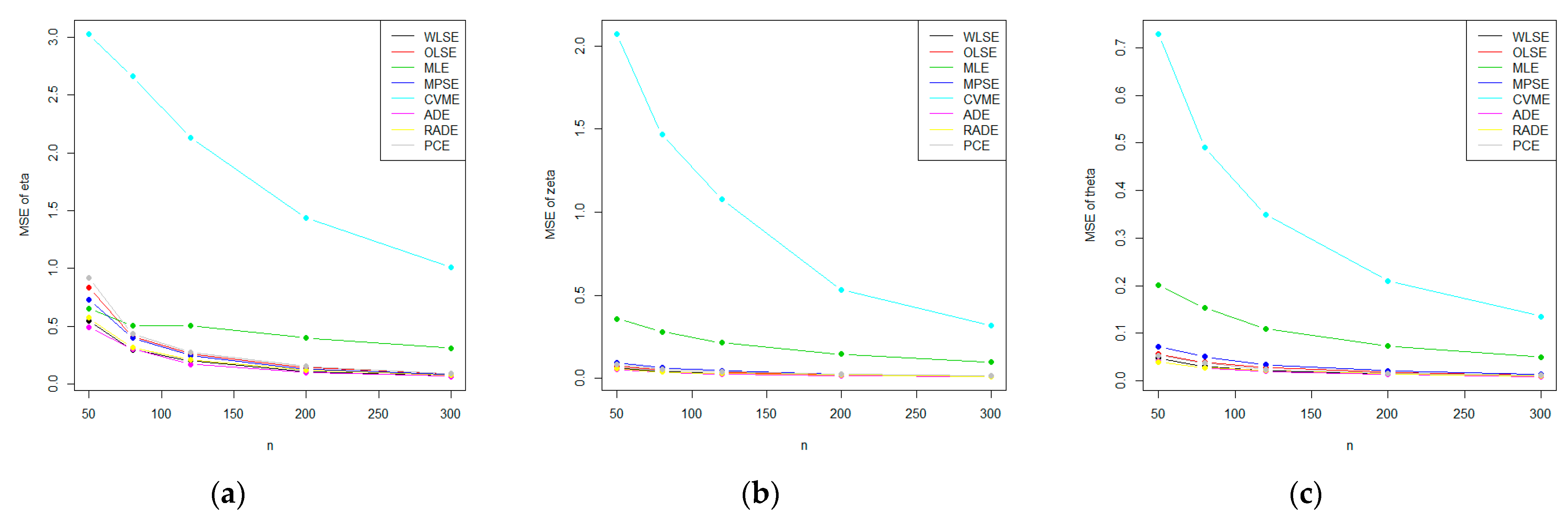
In this section, we estimate the E-NPF parameters $\eta$, $\zeta ,$and $\theta$ under complete samples using the MLE method.

Let $x_1,x_2, \dots ,x_n$ be a random sample of size n from the E-NPF distribution; if in the type II censoring scheme we observe only the first $r$ order statistics, then the likelihood function of $X$, $L^{*}\left(\Theta \right)$ takes the form

$$L^{*}\left(\Theta \right)=C {{\displaystyle \prod }}_{i=1}^{r }f\left(x_{i:r:n}\right){\left[1-F\left(x_{r:r:n}\right)\right]}^{n-r}, x_{1:r:n}\le x_{2:r:n}\le \cdots \le x_{r:r:n},$$

where $C$ is a constant that does not depend on the parameters and $x_{1:r:n}$, $x_{2:r:n}$, $\dots$, $x_{r:r:n}$ are the censored data. The log-likelihood function without the constant term can be written as follows:

$$\begin{gathered} L^{*}\left(\Theta \right)={\theta }^r{\zeta }^r{\left(1+\eta \right)}^r{\left[1-{\left(1-{\left(\frac{1-x_r}{1+\eta x_r}\right)}^{\zeta }\right)}^{\theta }\right]}^{n-r} \\ \times {{\displaystyle \prod }}_{i=1}^{r }\frac{{\left(1-x_i\right)}^{\zeta -1}}{{\left(1+\eta x_i\right)}^{\zeta +1}}{\left(1-{\left(\frac{1-x_i}{1+\eta x_i}\right)}^{\zeta }\right)}^{\theta -1}. \end{gathered}$$

The log-likelihood function, ${\ell }^{*}\left(\Theta \right)=\log L^{*}\left(\Theta \right)$, of $X$ is

$$\begin{gathered} {\ell }^{*}\left(\Theta \right)=r \log \theta +r \log \zeta +r \log \left(1+\eta \right)+\left(\zeta -1\right){\displaystyle \sum }_{i=1}^r\log \left(1-x_i\right) \\ -\left(\zeta +1\right){\displaystyle \sum }_{i=1}^r\log \left(1+\eta x_i\right)+\left(\theta -1\right){\displaystyle \sum }_{i=1}^r\log \left[1-{\left(\frac{1-x_i}{1+\eta x_i}\right)}^{\zeta }\right] \\ +\left(n-r\right)\log \left[1-{\left(1-{\left(\frac{1-x_r}{1+\eta x_r}\right)}^{\zeta }\right)}^{\theta }\right]. \end{gathered}$$

(26)

By taking partial derivatives of Equation (26), we get

$$\begin{gathered} \frac{\partial {\ell }^{*}\left(\Theta \right)}{\partial \eta }=\frac{r}{1+\eta }-\left(\zeta +1\right){\displaystyle \sum }_{i=1}^r\frac{x_i}{1+\eta x_i }+\zeta \left(\theta -1\right){\displaystyle \sum }_{i=1}^r\frac{x_i{\left(1-x_i\right)}^{\zeta }{\left(1+\eta x_i\right)}^{-\zeta -1}}{1-{\left(\frac{1-x_i}{1+\eta x_i}\right)}^{\zeta }} \\ -\theta \zeta \left(n-r\right)x_r{\left(1-x_r\right)}^{\zeta }{\left(1+\eta x_r\right)}^{-\zeta -1}\frac{{\left(1-{\left(\frac{1-x_r}{1+\eta x_r}\right)}^{\zeta }\right)}^{\theta -1}}{1-{\left(1-{\left(\frac{1-x_r}{1+\eta x_r}\right)}^{\zeta }\right)}^{\theta }}, \\ \frac{\partial {\ell }^{*}\left(\Theta \right)}{\partial \zeta }=\frac{r}{\zeta }+{\displaystyle \sum }_{i=1}^r\log \left(\frac{1-x_i}{1+\eta x_i }\right)-\left(\theta -1\right){\displaystyle \sum }_{i=1}^r\frac{{\left(\frac{1-x_i}{1+\eta x_i}\right)}^{\zeta }}{1-{\left(\frac{1-x_i}{1+\eta x_i}\right)}^{\zeta }}\log \left(\frac{1-x_i}{1+\eta x_i}\right) \\ +\theta \left(n-r\right)\log \left(\frac{1-x_r}{1+\eta x_r}\right)\frac{{\left(\frac{1-x_r}{1+\eta x_r}\right)}^{\zeta }{\left(1-{\left(\frac{1-x_r}{1+\eta x_r}\right)}^{\zeta }\right)}^{\theta -1}}{1-{\left(1-{\left(\frac{1-x_r}{1+\eta x_r}\right)}^{\zeta }\right)}^{\theta }} \\ \mathrm{and}\frac{\partial {\ell }^{*}\left(\Theta \right)}{\partial \theta }=\frac{r}{\theta }+{\displaystyle \sum }_{i=1}^r\log \left[1-{\left(\frac{1-x_i}{1+\eta x_i }\right)}^{\zeta }\right] \\ -\left(n-r\right)\log \left[1-{\left(\frac{1-x_r}{1+\eta x_r}\right)}^{\zeta }\right]\frac{{\left(1-{\left(\frac{1-x_r}{1+\eta x_r}\right)}^{\zeta }\right)}^{\theta }}{1-{\left(1-{\left(\frac{1-x_r}{1+\eta x_r}\right)}^{\zeta }\right)}^{\theta }} \end{gathered}$$

The type II censored ML estimators (CMLE) ${\widehat{\eta }}_{CMLE}$, , and of the E-NPF distribution can be obtained by maximizing Equation (26) or by solving the above equations simultaneously by any numerical method as in Section 4.1.1.

5. Simulation Study

In this section, we perform the simulation study of the E-NPF distribution for complete samples using eight estimation methods and under the type II censored samples for the MLE method.

5.1. Simulation Results under Complete Samples

In this section, the performance of the estimates is discussed by the following algorithm.

Step 1:

A random sample $x_1, x_2, \dots x_n$ of sizes $n=50, 80, 120, 200$, and $300$ are generated from the QF in Equation (14).

Step 2:

The required results are obtained based on 36 combinations of the parameters $\eta =\left\{-0.50, 0.75, 1.50, 4.00\right\}, \zeta =\left\{0.50, 1.75, 3.00\right\}$ and $\theta =\left\{0.40, 1.60, 2.75\right\}.$

Step 3:

Each sample is replicated $N=5000$ times.

Step 4:

Results of the average of absolute value of biases ($\left|Bias\left(\widehat{\Theta }\right)\right|$), $\left|Bias\left(\widehat{\Theta }\right)\right|=$ $\frac{1}{N}{\displaystyle \sum }_{i=1}^N\left|\widehat{\Theta }-\Theta \right|,$ the average of mean square errors (MSE), $MSE=\frac{1}{N}{\displaystyle \sum }_{i=1}^N{\left(\widehat{\Theta }-\Theta \right)}^2$, and the average of mean relative errors (MRE), $MRE=\frac{\frac{1}{N}{{\displaystyle \sum }}_{i=1}^N\left|\widehat{\Theta }-\Theta \right|}{\Theta }$, where $\Theta ={\left(\eta ,\zeta , \theta \right)}^T,$are computed for the 36 combinations; to save more space, we present just the result of 4 combinations in

Table 3. Simulated results of the E-NPF distribution for $\Theta ={\left(\eta =-0.50,\zeta =0.05,\theta =0.40\right)}^T$.

$\mathit{n}$	$\mathit{E}\mathit{s}\mathit{t}.$	$\mathit{E}\mathit{s}\mathit{t}. \mathit{P}\mathit{a}\mathit{r}.$	$\mathit{W}\mathit{L}\mathit{S}\mathit{E}$	$\mathit{O}\mathit{L}\mathit{S}\mathit{E}$	$\mathit{M}\mathit{L}\mathit{E}$	$\mathit{M}\mathit{P}\mathit{S}\mathit{E}$	$\mathit{C}\mathit{V}\mathit{M}\mathit{E}$	$\mathit{A}\mathit{D}\mathit{E}$	$\mathit{R}\mathit{A}\mathit{D}\mathit{E}$	$\mathit{P}\mathit{C}\mathit{E}$
50	$\left|BIAS\right|$	$\widehat{\eta }$	0.22949{2}	0.25491{5}	0.19893{1}	0.25592{6}	0.59344{8}	0.23115{3}	0.24367{4}	0.31888{7}
		$\widehat{\zeta }$	0.04667{3}	0.05170{5}	0.18196{7}	0.06960{6}	0.31282{8}	0.04117{1}	0.04246{2}	0.04977{4}
		$\widehat{\theta }$	0.02636{3}	0.02929{4}	0.05176{7}	0.03909{6}	0.10345{8}	0.02486{2}	0.02304{1}	0.03038{5}
	$MSE$	$\widehat{\eta }$	0.13184{3}	0.16396{6}	0.06754{1}	0.15261{5}	0.91318{8}	0.12109{2}	0.13419{4}	0.35193{7}
		$\widehat{\zeta }$	0.00677{3}	0.00845{4}	0.10140{7}	0.01070{6}	0.42939{8}	0.00573{1}	0.00587{2}	0.00995{5}
		$\widehat{\theta }$	0.00223{3}	0.00275{4}	0.00450{7}	0.00355{5.5}	0.02340{8}	0.00208{1}	0.00213{2}	0.00355{5.5}
	$MRE$	$\widehat{\eta }$	−0.45897{7}	−0.50983{4}	−0.39786{8}	−0.51184{3}	−1.18688{1}	−0.46229{6}	−0.48734{5}	−0.63776{2}
		$\widehat{\zeta }$	0.09333{3}	0.10340{5}	0.36391{7}	0.13921{6}	0.62564{8}	0.08234{1}	0.08492{2}	0.09953{4}
		$\widehat{\theta }$	0.06590{3}	0.07323{4}	0.12941{7}	0.09772{6}	0.25861{8}	0.06214{2}	0.05759{1}	0.07596{5}
	${{\displaystyle \sum }}^{}Ranks$		30{3}	41{4}	52{7}	49.5{6}	65{8}	19{1}	23{2}	44.5{5}
80	$\left|BIAS\right|$	$\widehat{\eta }$	0.17731{3}	0.18881{5}	0.15427{1}	0.19846{6}	0.43540{8}	0.17521{2}	0.18167{4}	0.23895{7}
		$\widehat{\zeta }$	0.03774{3}	0.04176{4}	0.12121{7}	0.05495{6}	0.18780{8}	0.03414{2}	0.03376{1}	0.04447{5}
		$\widehat{\theta }$	0.02112{2}	0.02396{4}	0.04053{7}	0.03054{6}	0.07637{8}	0.02144{3}	0.01970{1}	0.02658{5}
	$MSE$	$\widehat{\eta }$	0.06778{4}	0.07756{5}	0.03938{1}	0.08202{6}	0.51767{8}	0.06301{2}	0.06548{3}	0.15423{7}
		$\widehat{\zeta }$	0.00463{3}	0.00564{4}	0.03587{7}	0.00699{5}	0.12950{8}	0.00403{2}	0.00375{1}	0.00770{6}
		$\widehat{\theta }$	0.00149{1}	0.00185{4}	0.00267{7}	0.00229{5}	0.01157{8}	0.00151{2}	0.00160{3}	0.00260{6}
	$MRE$	$\widehat{\eta }$	−0.35462{6}	−0.37762{4}	−0.30854{8}	−0.39692{3}	−0.8708{1}	−0.35042{7}	−0.36334{5}	−0.4779{2}
		$\widehat{\zeta }$	0.07548{3}	0.08352{4}	0.24243{7}	0.10990{6}	0.37560{8}	0.06828{2}	0.06752{1}	0.08895{5}
		$\widehat{\theta }$	0.05281{2}	0.05990{4}	0.10134{7}	0.07635{6}	0.19092{8}	0.05359{3}	0.04925{1}	0.06644{5}
	${{\displaystyle \sum }}^{}Ranks$		27{3}	38{4}	52{7}	49{6}	65{8}	25{2}	20{1}	48{5}
120	$\left|BIAS\right|$	$\widehat{\eta }$	0.14157{3}	0.15071{5}	0.12488{1}	0.15701{6}	0.33864{8}	0.13949{2}	0.14476{4}	0.18448{7}
		$\widehat{\zeta }$	0.03095{3}	0.03374{4}	0.09034{7}	0.04572{6}	0.13792{8}	0.02903{2}	0.02884{1}	0.03617{5}
		$\widehat{\theta }$	0.01823{3}	0.01927{4}	0.03334{7}	0.02489{6}	0.06217{8}	0.01704{1}	0.01706{2}	0.02058{5}
	$MSE$	$\widehat{\eta }$	0.03753{3}	0.04486{5}	0.02492{1}	0.04625{6}	0.29530{8}	0.03533{2}	0.03942{4}	0.07910{7}
		$\widehat{\zeta }$	0.00322{3}	0.00387{4}	0.01580{7}	0.00489{5}	0.05979{8}	0.00296{2}	0.00280{1}	0.00551{6}
		$\widehat{\theta }$	0.00109{2}	0.00124{4}	0.00178{7}	0.00158{5}	0.00718{8}	0.00102{1}	0.00117{3}	0.00168{6}
	$MRE$	$\widehat{\eta }$	−0.28313{6}	−0.30143{4}	−0.24976{8}	−0.31402{3}	−0.67728{1}	−0.27899{7}	−0.28951{5}	−0.36896{2}
		$\widehat{\zeta }$	0.06189{3}	0.06748{4}	0.18069{7}	0.09144{6}	0.27583{8}	0.05807{2}	0.05768{1}	0.07234{5}
		$\widehat{\theta }$	0.04558{3}	0.04819{4}	0.08336{7}	0.06223{6}	0.15542{8}	0.04261{1}	0.04266{2}	0.05144{5}
	${{\displaystyle \sum }}^{}Ranks$		29{3}	38{4}	52{7}	49{6}	65{8}	20{1}	23{2}	48{5}
200	$\left|BIAS\right|$	$\widehat{\eta }$	0.10664{3}	0.11928{5}	0.09892{1}	0.12024{6}	0.23829{8}	0.10411{2}	0.11143{4}	0.13639{7}
		$\widehat{\zeta }$	0.02358{2}	0.02825{4}	0.06684{7}	0.03499{6}	0.09182{8}	0.02231{1}	0.02393{3}	0.03000{5}
		$\widehat{\theta }$	0.01428{3}	0.01553{4}	0.02558{7}	0.01909{6}	0.04646{8}	0.01396{2}	0.01361{1}	0.01745{5}
	$MSE$	$\widehat{\eta }$	0.02023{3}	0.02580{6}	0.01563{1}	0.02485{5}	0.12311{8}	0.01853{2}	0.02153{4}	0.03900{7}
		$\widehat{\zeta }$	0.00193{3}	0.00270{4}	0.00792{7}	0.00300{5}	0.01711{8}	0.00179{1}	0.00192{2}	0.00374{6}
		$\widehat{\theta }$	0.00069{2}	0.00081{4}	0.00104{6}	0.00095{5}	0.00374{8}	0.00067{1}	0.00075{3}	0.00117{7}
	$MRE$	$\widehat{\eta }$	−0.21328{6}	−0.23857{4}	−0.19785{8}	−0.24047{3}	−0.47659{1}	−0.20822{7}	−0.22286{5}	−0.27279{2}
		$\widehat{\zeta }$	0.04715{2}	0.05650{4}	0.13367{7}	0.06998{6}	0.18363{8}	0.04463{1}	0.04785{3}	0.05999{5}
		$\widehat{\theta }$	0.03569{3}	0.03882{4}	0.06396{7}	0.04771{6}	0.11615{8}	0.03490{2}	0.03403{1}	0.04363{5}
	${{\displaystyle \sum }}^{}Ranks$		27{3}	39{4}	51{7}	48{5}	65{8}	19{1}	26{2}	49{6}
300	$\left|BIAS\right|$	$\widehat{\eta }$	0.08835{3}	0.09392{5}	0.07939{1}	0.09739{6}	0.18183{8}	0.08621{2}	0.09360{4}	0.11021{7}
		$\widehat{\zeta }$	0.01974{2}	0.02301{4}	0.05371{7}	0.02904{6}	0.07244{8}	0.01876{1}	0.01985{3}	0.02533{5}
		$\widehat{\theta }$	0.01189{3}	0.01239{4}	0.02043{7}	0.01573{6}	0.03646{8}	0.01102{1}	0.01173{2}	0.01472{5}
	$MSE$	$\widehat{\eta }$	0.01318{3}	0.01549{5}	0.01010{1}	0.01596{6}	0.06384{8}	0.01270{2}	0.01515{4}	0.02281{7}
		$\widehat{\zeta }$	0.00138{3}	0.00186{4}	0.00510{7}	0.00213{5}	0.00970{8}	0.00128{1}	0.00135{2}	0.00263{6}
		$\widehat{\theta }$	0.00048{2}	0.00054{3}	0.00072{6}	0.00067{5}	0.00221{8}	0.00044{1}	0.00056{4}	0.00084{7}
	$MRE$	$\widehat{\eta }$	−0.1767{6}	−0.18785{4}	−0.15877{8}	−0.19478{3}	−0.36365{1}	−0.17241{7}	−0.18719{5}	−0.22042{2}
		$\widehat{\zeta }$	0.03948{2}	0.04601{4}	0.10742{7}	0.05807{6}	0.14487{8}	0.03752{1}	0.03971{3}	0.05066{5}
		$\widehat{\theta }$	0.02973{3}	0.03096{4}	0.05108{7}	0.03932{6}	0.09115{8}	0.02755{1}	0.02934{2}	0.03680{5}
	${\displaystyle \sum }Ranks$		27{2}	37{4}	51{7}	49{5.5}	65{8}	17{1}	29{3}	49{5.5}

,

Table 4. Simulated results of the E-NPF distribution for $\Theta ={\left(\eta =-0.50,\zeta =3.00,\theta =2.75\right)}^T$.

$\mathit{n}$	$\mathit{E}\mathit{s}\mathit{t}.$	$\mathit{E}\mathit{s}\mathit{t}. \mathit{P}\mathit{a}\mathit{r}.$	$\mathit{W}\mathit{L}\mathit{S}\mathit{E}$	$\mathit{O}\mathit{L}\mathit{S}\mathit{E}$	$\mathit{M}\mathit{L}\mathit{E}$	$\mathit{M}\mathit{P}\mathit{S}\mathit{E}$	$\mathit{C}\mathit{V}\mathit{M}\mathit{E}$	$\mathit{A}\mathit{D}\mathit{E}$	$\mathit{R}\mathit{A}\mathit{D}\mathit{E}$	$\mathit{P}\mathit{C}\mathit{E}$
50	$\left|BIAS\right|$	$\widehat{\eta }$	${0.12979}^{\left\{2\right\}}$	${0.14559}^{\left\{5\right\}}$	${0.16943}^{\left\{7\right\}}$	${0.16244}^{\left\{6\right\}}$	${0.52954}^{\left\{8\right\}}$	${0.12226}^{\left\{1\right\}}$	${0.13258}^{\left\{3\right\}}$	${0.14036}^{\left\{4\right\}}$
		$\widehat{\zeta }$	${0.24022}^{\left\{3\right\}}$	${0.25187}^{\left\{4\right\}}$	${1.08184}^{\left\{7\right\}}$	${0.35420}^{\left\{6\right\}}$	${1.53271}^{\left\{8\right\}}$	${0.21467}^{\left\{1\right\}}$	${0.23337}^{\left\{2\right\}}$	${0.25346}^{\left\{5\right\}}$
		$\widehat{\theta }$	${0.18768}^{\left\{3\right\}}$	${0.21042}^{\left\{4\right\}}$	${0.33180}^{\left\{7\right\}}$	${0.28515}^{\left\{6\right\}}$	${1.31026}^{\left\{8\right\}}$	${0.16952}^{\left\{2\right\}}$	${0.15364}^{\left\{1\right\}}$	${0.23660}^{\left\{5\right\}}$
	$MSE$	$\widehat{\eta }$	${0.04480}^{\left\{3\right\}}$	${0.05842}^{\left\{6\right\}}$	${0.04339}^{\left\{2\right\}}$	${0.06358}^{\left\{7\right\}}$	${0.61461}^{\left\{8\right\}}$	${0.04073}^{\left\{1\right\}}$	${0.04623}^{\left\{4\right\}}$	${0.05168}^{\left\{5\right\}}$
		$\widehat{\zeta }$	${0.21601}^{\left\{3\right\}}$	${0.24565}^{\left\{5\right\}}$	${2.08797}^{\left\{7\right\}}$	${0.33088}^{\left\{6\right\}}$	${3.48991}^{\left\{8\right\}}$	${0.18998}^{\left\{1\right\}}$	${0.20774}^{\left\{2\right\}}$	${0.23431}^{\left\{4\right\}}$
		$\widehat{\theta }$	${0.13709}^{\left\{3\right\}}$	${0.17231}^{\left\{4\right\}}$	${0.18137}^{\left\{6\right\}}$	${0.22355}^{\left\{7\right\}}$	${2.83494}^{\left\{8\right\}}$	${0.11965}^{\left\{1\right\}}$	${0.12364}^{\left\{2\right\}}$	${0.17976}^{\left\{5\right\}}$
	$MRE$	$\widehat{\eta }$	$-{0.25959}^{\left\{7\right\}}$	$-{0.29119}^{\left\{4\right\}}$	$-{0.33886}^{\left\{2\right\}}$	$-{0.32488}^{\left\{3\right\}}$	$-{1.05908}^{\left\{1\right\}}$	$-{0.24453}^{\left\{8\right\}}$	$-{0.26515}^{\left\{6\right\}}$	$-{0.28072}^{\left\{5\right\}}$
		$\widehat{\zeta }$	${0.08007}^{\left\{3\right\}}$	${0.08396}^{\left\{4\right\}}$	${0.36061}^{\left\{7\right\}}$	${0.11807}^{\left\{6\right\}}$	${0.51090}^{\left\{8\right\}}$	${0.07156}^{\left\{1\right\}}$	${0.07779}^{\left\{2\right\}}$	${0.08449}^{\left\{5\right\}}$
		$\widehat{\theta }$	${0.06825}^{\left\{3\right\}}$	${0.07652}^{\left\{4\right\}}$	${0.12066}^{\left\{7\right\}}$	${0.10369}^{\left\{6\right\}}$	${0.47646}^{\left\{8\right\}}$	${0.06164}^{\left\{2\right\}}$	${0.05587}^{\left\{1\right\}}$	${0.08604}^{\left\{5\right\}}$
	${{\displaystyle \sum }}^{}Ranks$		${30}^{\left\{3\right\}}$	${40}^{\left\{4\right\}}$	${52}^{\left\{6\right\}}$	${53}^{\left\{7\right\}}$	${65}^{\left\{8\right\}}$	${18}^{\left\{1\right\}}$	${23}^{\left\{2\right\}}$	${43}^{\left\{5\right\}}$
80	$\left|BIAS\right|$	$\widehat{\eta }$	${0.09688}^{\left\{2\right\}}$	${0.11300}^{\left\{5\right\}}$	${0.13982}^{\left\{7\right\}}$	${0.12331}^{\left\{6\right\}}$	${0.46150}^{\left\{8\right\}}$	${0.09236}^{\left\{1\right\}}$	${0.10297}^{\left\{3\right\}}$	${0.10608}^{\left\{4\right\}}$
		$\widehat{\zeta }$	${0.18949}^{\left\{2\right\}}$	${0.21166}^{\left\{5\right\}}$	${0.85813}^{\left\{7\right\}}$	${0.29268}^{\left\{6\right\}}$	${1.39834}^{\left\{8\right\}}$	${0.17417}^{\left\{1\right\}}$	${0.20374}^{\left\{3\right\}}$	${0.20588}^{\left\{4\right\}}$
		$\widehat{\theta }$	${0.15388}^{\left\{3\right\}}$	${0.17170}^{\left\{4\right\}}$	${0.26269}^{\left\{7\right\}}$	${0.23382}^{\left\{6\right\}}$	${1.09522}^{\left\{8\right\}}$	${0.14016}^{\left\{2\right\}}$	${0.13275}^{\left\{1\right\}}$	${0.19536}^{\left\{5\right\}}$
	$MSE$	$\widehat{\eta }$	${0.02400}^{\left\{2\right\}}$	${0.03399}^{\left\{6\right\}}$	${0.02960}^{\left\{5\right\}}$	${0.03622}^{\left\{7\right\}}$	${0.45408}^{\left\{8\right\}}$	${0.02188}^{\left\{1\right\}}$	${0.02611}^{\left\{3\right\}}$	${0.02915}^{\left\{4\right\}}$
		$\widehat{\zeta }$	${0.14473}^{\left\{2\right\}}$	${0.17939}^{\left\{5\right\}}$	${1.39876}^{\left\{7\right\}}$	${0.23343}^{\left\{6\right\}}$	${3.04521}^{\left\{8\right\}}$	${0.12981}^{\left\{1\right\}}$	${0.15416}^{\left\{3\right\}}$	${0.16151}^{\left\{4\right\}}$
		$\widehat{\theta }$	${0.09709}^{\left\{3\right\}}$	${0.11684}^{\left\{5\right\}}$	${0.11149}^{\left\{4\right\}}$	${0.15147}^{\left\{7\right\}}$	${2.16423}^{\left\{8\right\}}$	${0.08582}^{\left\{1\right\}}$	${0.09124}^{\left\{2\right\}}$	${0.12781}^{\left\{6\right\}}$
	$MRE$	$\widehat{\eta }$	$-{0.19375}^{\left\{7\right\}}$	$-{0.22600}^{\left\{4\right\}}$	$-{0.27963}^{\left\{2\right\}}$	$-{0.24661}^{\left\{3\right\}}$	$-{0.92299}^{\left\{1\right\}}$	$-{0.18472}^{\left\{8\right\}}$	$-{0.20594}^{\left\{6\right\}}$	$-{0.21216}^{\left\{5\right\}}$
		$\widehat{\zeta }$	${0.06316}^{\left\{2\right\}}$	${0.07055}^{\left\{5\right\}}$	${0.28604}^{\left\{7\right\}}$	${0.09756}^{\left\{6\right\}}$	${0.46611}^{\left\{8\right\}}$	${0.05806}^{\left\{1\right\}}$	${0.06791}^{\left\{3\right\}}$	${0.06863}^{\left\{4\right\}}$
		$\widehat{\theta }$	${0.05596}^{\left\{3\right\}}$	${0.06244}^{\left\{4\right\}}$	${0.09552}^{\left\{7\right\}}$	${0.08502}^{\left\{6\right\}}$	${0.39826}^{\left\{8\right\}}$	${0.05097}^{\left\{2\right\}}$	${0.04827}^{\left\{1\right\}}$	${0.07104}^{\left\{5\right\}}$
	${{\displaystyle \sum }}^{}Ranks$		${26}^{\left\{3\right\}}$	${43}^{\left\{5\right\}}$	${53}^{\left\{6.5\right\}}$	${53}^{\left\{6.5\right\}}$	${65}^{\left\{8\right\}}$	${18}^{\left\{1\right\}}$	${25}^{\left\{2\right\}}$	${41}^{\left\{4\right\}}$
120	$\left|BIAS\right|$	$\widehat{\eta }$	${0.07626}^{\left\{2\right\}}$	${0.08634}^{\left\{5\right\}}$	${0.11562}^{\left\{7\right\}}$	${0.09305}^{\left\{6\right\}}$	${0.40541}^{\left\{8\right\}}$	${0.07383}^{\left\{1\right\}}$	${0.08240}^{\left\{3\right\}}$	${0.08336}^{\left\{4\right\}}$
		$\widehat{\zeta }$	${0.15843}^{\left\{2\right\}}$	${0.17740}^{\left\{5\right\}}$	${0.67780}^{\left\{7\right\}}$	${0.24322}^{\left\{6\right\}}$	${1.24222}^{\left\{8\right\}}$	${0.14885}^{\left\{1\right\}}$	${0.16879}^{\left\{3\right\}}$	${0.17581}^{\left\{4\right\}}$
		$\widehat{\theta }$	${0.13001}^{\left\{3\right\}}$	${0.14300}^{\left\{4\right\}}$	${0.21290}^{\left\{7\right\}}$	${0.19094}^{\left\{6\right\}}$	${0.96309}^{\left\{8\right\}}$	${0.12004}^{\left\{2\right\}}$	${0.11100}^{\left\{1\right\}}$	${0.15496}^{\left\{5\right\}}$
	$MSE$	$\widehat{\eta }$	${0.01414}^{\left\{2\right\}}$	${0.01898}^{\left\{5\right\}}$	${0.02067}^{\left\{7\right\}}$	${0.01912}^{\left\{6\right\}}$	${0.34150}^{\left\{8\right\}}$	${0.01313}^{\left\{1\right\}}$	${0.01627}^{\left\{3\right\}}$	${0.01652}^{\left\{4\right\}}$
		$\widehat{\zeta }$	${0.10536}^{\left\{2\right\}}$	${0.12796}^{\left\{5\right\}}$	${0.90465}^{\left\{7\right\}}$	${0.16222}^{\left\{6\right\}}$	${2.53541}^{\left\{8\right\}}$	${0.09502}^{\left\{1\right\}}$	${0.11142}^{\left\{3\right\}}$	${0.11779}^{\left\{4\right\}}$
		$\widehat{\theta }$	${0.06903}^{\left\{3\right\}}$	${0.08560}^{\left\{6\right\}}$	${0.07241}^{\left\{4\right\}}$	${0.10479}^{\left\{7\right\}}$	${1.74908}^{\left\{8\right\}}$	${0.06287}^{\left\{1\right\}}$	${0.06535}^{\left\{2\right\}}$	${0.08549}^{\left\{5\right\}}$
	$MRE$	$\widehat{\eta }$	$-{0.15252}^{\left\{7\right\}}$	$-{0.17269}^{\left\{4\right\}}$	$-{0.23123}^{\left\{2\right\}}$	$-{0.18611}^{\left\{3\right\}}$	$-{0.81083}^{\left\{1\right\}}$	$-{0.14766}^{\left\{8\right\}}$	$-{0.16480}^{\left\{6\right\}}$	$-{0.16672}^{\left\{5\right\}}$
		$\widehat{\zeta }$	${0.05281}^{\left\{2\right\}}$	${0.05913}^{\left\{5\right\}}$	${0.22593}^{\left\{7\right\}}$	${0.08107}^{\left\{6\right\}}$	${0.41407}^{\left\{8\right\}}$	${0.04962}^{\left\{1\right\}}$	${0.05626}^{\left\{3\right\}}$	${0.05860}^{\left\{4\right\}}$
		$\widehat{\theta }$	${0.04728}^{\left\{3\right\}}$	${0.05200}^{\left\{4\right\}}$	${0.07742}^{\left\{7\right\}}$	${0.06943}^{\left\{6\right\}}$	${0.35022}^{\left\{8\right\}}$	${0.04365}^{\left\{2\right\}}$	${0.04037}^{\left\{1\right\}}$	${0.05635}^{\left\{5\right\}}$
	${{\displaystyle \sum }}^{}Ranks$		${26}^{\left\{3\right\}}$	${43}^{\left\{5\right\}}$	${55}^{\left\{7\right\}}$	${52}^{\left\{6\right\}}$	${65}^{\left\{8\right\}}$	${18}^{\left\{1\right\}}$	${25}^{\left\{2\right\}}$	${40}^{\left\{4\right\}}$
200	$\left|BIAS\right|$	$\widehat{\eta }$	${0.05770}^{\left\{1\right\}}$	${0.06866}^{\left\{6\right\}}$	${0.09188}^{\left\{7\right\}}$	${0.06779}^{\left\{5\right\}}$	${0.31533}^{\left\{8\right\}}$	${0.05846}^{\left\{2\right\}}$	${0.06428}^{\left\{4\right\}}$	${0.06416}^{\left\{3\right\}}$
		$\widehat{\zeta }$	${0.12451}^{\left\{1\right\}}$	${0.14279}^{\left\{5\right\}}$	${0.50172}^{\left\{7\right\}}$	${0.18437}^{\left\{6\right\}}$	${1.05528}^{\left\{8\right\}}$	${0.12901}^{\left\{2\right\}}$	${0.14109}^{\left\{3\right\}}$	${0.14211}^{\left\{4\right\}}$
		$\widehat{\theta }$	${0.09473}^{\left\{2\right\}}$	${0.11525}^{\left\{4\right\}}$	${0.16533}^{\left\{7\right\}}$	${0.14666}^{\left\{6\right\}}$	${0.73334}^{\left\{8\right\}}$	${0.09487}^{\left\{3\right\}}$	${0.08544}^{\left\{1\right\}}$	${0.12004}^{\left\{5\right\}}$
	$MSE$	$\widehat{\eta }$	${0.00777}^{\left\{1\right\}}$	${0.01188}^{\left\{6\right\}}$	${0.01306}^{\left\{7\right\}}$	${0.01078}^{\left\{5\right\}}$	${0.19926}^{\left\{8\right\}}$	${0.00825}^{\left\{2\right\}}$	${0.01025}^{\left\{4\right\}}$	${0.00933}^{\left\{3\right\}}$
		$\widehat{\zeta }$	${0.06763}^{\left\{1\right\}}$	${0.08910}^{\left\{5\right\}}$	${0.47292}^{\left\{7\right\}}$	${0.10125}^{\left\{6\right\}}$	${1.94905}^{\left\{8\right\}}$	${0.07006}^{\left\{2\right\}}$	${0.08082}^{\left\{4\right\}}$	${0.07923}^{\left\{3\right\}}$
		$\widehat{\theta }$	${0.03932}^{\left\{1\right\}}$	${0.05587}^{\left\{6\right\}}$	${0.04399}^{\left\{4\right\}}$	${0.06452}^{\left\{7\right\}}$	${1.06839}^{\left\{8\right\}}$	${0.04104}^{\left\{2.5\right\}}$	${0.04104}^{\left\{2.5\right\}}$	${0.05219}^{\left\{5\right\}}$
	$MRE$	$\widehat{\eta }$	$-{0.11539}^{\left\{8\right\}}$	$-{0.13733}^{\left\{3\right\}}$	$-{0.18375}^{\left\{2\right\}}$	$-{0.13559}^{\left\{4\right\}}$	$-{0.63066}^{\left\{1\right\}}$	$-{0.11692}^{\left\{7\right\}}$	$-{0.12856}^{\left\{5\right\}}$	$-{0.12832}^{\left\{6\right\}}$
		$\widehat{\zeta }$	${0.04150}^{\left\{1\right\}}$	${0.04760}^{\left\{5\right\}}$	${0.16724}^{\left\{7\right\}}$	${0.06146}^{\left\{6\right\}}$	${0.35176}^{\left\{8\right\}}$	${0.04300}^{\left\{2\right\}}$	${0.04703}^{\left\{3\right\}}$	${0.04737}^{\left\{4\right\}}$
		$\widehat{\theta }$	${0.03445}^{\left\{2\right\}}$	${0.04191}^{\left\{4\right\}}$	${0.06012}^{\left\{7\right\}}$	${0.05333}^{\left\{6\right\}}$	${0.26667}^{\left\{8\right\}}$	${0.03450}^{\left\{3\right\}}$	${0.03107}^{\left\{1\right\}}$	${0.04365}^{\left\{5\right\}}$
	${{\displaystyle \sum }}^{}Ranks$		${18}^{\left\{1\right\}}$	${44}^{\left\{5\right\}}$	${55}^{\left\{7\right\}}$	${51}^{\left\{6\right\}}$	${65}^{\left\{8\right\}}$	${25.5}^{\left\{2\right\}}$	${27.5}^{\left\{3\right\}}$	${38}^{\left\{4\right\}}$
300	$\left|BIAS\right|$	$\widehat{\eta }$	${0.04663}^{\left\{1\right\}}$	${0.05602}^{\left\{6\right\}}$	${0.07341}^{\left\{7\right\}}$	${0.05094}^{\left\{4\right\}}$	${0.25807}^{\left\{8\right\}}$	${0.04725}^{\left\{2\right\}}$	${0.05124}^{\left\{5\right\}}$	${0.04901}^{\left\{3\right\}}$
		$\widehat{\zeta }$	${0.10493}^{\left\{1\right\}}$	${0.12490}^{\left\{5\right\}}$	${0.38948}^{\left\{7\right\}}$	${0.14556}^{\left\{6\right\}}$	${0.89668}^{\left\{8\right\}}$	${0.10703}^{\left\{2\right\}}$	${0.11386}^{\left\{4\right\}}$	${0.10855}^{\left\{3\right\}}$
		$\widehat{\theta }$	${0.08280}^{\left\{3\right\}}$	${0.09077}^{\left\{4\right\}}$	${0.13279}^{\left\{7\right\}}$	${0.12087}^{\left\{6\right\}}$	${0.60461}^{\left\{8\right\}}$	${0.07890}^{\left\{1\right\}}$	${0.07931}^{\left\{2\right\}}$	${0.09579}^{\left\{5\right\}}$
	$MSE$	$\widehat{\eta }$	${0.00513}^{\left\{1\right\}}$	${0.00758}^{\left\{6\right\}}$	${0.00848}^{\left\{7\right\}}$	${0.00627}^{\left\{5\right\}}$	${0.13045}^{\left\{8\right\}}$	${0.00528}^{\left\{2\right\}}$	${0.00612}^{\left\{4\right\}}$	${0.00542}^{\left\{3\right\}}$
		$\widehat{\zeta }$	${0.04878}^{\left\{1\right\}}$	${0.06664}^{\left\{5\right\}}$	${0.27778}^{\left\{7\right\}}$	${0.06687}^{\left\{6\right\}}$	${1.50712}^{\left\{8\right\}}$	${0.05059}^{\left\{2\right\}}$	${0.05422}^{\left\{4\right\}}$	${0.05082}^{\left\{3\right\}}$
		$\widehat{\theta }$	${0.03040}^{\left\{3\right\}}$	${0.03624}^{\left\{6\right\}}$	${0.02792}^{\left\{1\right\}}$	${0.04385}^{\left\{7\right\}}$	${0.72788}^{\left\{8\right\}}$	${0.02803}^{\left\{2\right\}}$	${0.03250}^{\left\{4\right\}}$	${0.03494}^{\left\{5\right\}}$
	$MRE$	$\widehat{\eta }$	$-{0.09326}^{\left\{8\right\}}$	$-{0.11204}^{\left\{3\right\}}$	$-{0.14681}^{\left\{2\right\}}$	$-{0.10187}^{\left\{5\right\}}$	$-{0.51614}^{\left\{1\right\}}$	$-{0.09451}^{\left\{7\right\}}$	$-{0.10247}^{\left\{4\right\}}$	$-{0.09801}^{\left\{6\right\}}$
		$\widehat{\zeta }$	${0.03498}^{\left\{1\right\}}$	${0.04163}^{\left\{5\right\}}$	${0.12983}^{\left\{7\right\}}$	${0.04852}^{\left\{6\right\}}$	${0.29889}^{\left\{8\right\}}$	${0.03568}^{\left\{2\right\}}$	${0.03795}^{\left\{4\right\}}$	${0.03618}^{\left\{3\right\}}$
		$\widehat{\theta }$	${0.03011}^{\left\{3\right\}}$	${0.03301}^{\left\{4\right\}}$	${0.04829}^{\left\{7\right\}}$	${0.04395}^{\left\{6\right\}}$	${0.21986}^{\left\{8\right\}}$	${0.02869}^{\left\{1\right\}}$	${0.02884}^{\left\{2\right\}}$	${0.03483}^{\left\{5\right\}}$
	${{\displaystyle \sum }}^{}Ranks$		${22}^{\left\{2\right\}}$	${44}^{\left\{5\right\}}$	${52}^{\left\{7\right\}}$	${51}^{\left\{6\right\}}$	${65}^{\left\{8\right\}}$	${21}^{\left\{1\right\}}$	${33}^{\left\{3\right\}}$	${36}^{\left\{4\right\}}$

,

Table 5. Simulated results of the E-NPF distribution for $\Theta ={\left(\eta =0.75,\zeta =0.50,\theta =1.60\right)}^T$.

$\mathit{n}$	$\mathit{E}\mathit{s}\mathit{t}.$	$\mathit{E}\mathit{s}\mathit{t}. \mathit{P}\mathit{a}\mathit{r}.$	$\mathit{W}\mathit{L}\mathit{S}\mathit{E}$	$\mathit{O}\mathit{L}\mathit{S}\mathit{E}$	$\mathit{M}\mathit{L}\mathit{E}$	$\mathit{M}\mathit{P}\mathit{S}\mathit{E}$	$\mathit{C}\mathit{V}\mathit{M}\mathit{E}$	$\mathit{A}\mathit{D}\mathit{E}$	$\mathit{R}\mathit{A}\mathit{D}\mathit{E}$	$\mathit{P}\mathit{C}\mathit{E}$
50	$\left|BIAS\right|$	$\widehat{\eta }$	${0.73346}^{\left\{4\right\}}$	${0.83157}^{\left\{6\right\}}$	${0.47441}^{\left\{1\right\}}$	${0.70996}^{\left\{3\right\}}$	${1.80055}^{\left\{8\right\}}$	${0.68856}^{\left\{2\right\}}$	${0.78778}^{\left\{5\right\}}$	${0.86431}^{\left\{7\right\}}$
		$\widehat{\zeta }$	${0.03109}^{\left\{3\right\}}$	${0.03401}^{\left\{5\right\}}$	${0.08215}^{\left\{7\right\}}$	${0.04159}^{\left\{6\right\}}$	${0.12918}^{\left\{8\right\}}$	${0.02678}^{\left\{1\right\}}$	${0.02899}^{\left\{2\right\}}$	.${0.03272}^{\left\{4\right\}}$
		$\widehat{\theta }$	${0.22988}^{\left\{4\right\}}$	${0.24045}^{\left\{5\right\}}$	${0.18999}^{\left\{1\right\}}$	${0.30034}^{\left\{7\right\}}$	${0.80596}^{\left\{8\right\}}$	${0.19660}^{\left\{2\right\}}$	${0.24741}^{\left\{6\right\}}$	${0.21868}^{\left\{3\right\}}$
	$MSE$	$\widehat{\eta }$	${0.89062}^{\left\{3\right\}}$	${1.19085}^{\left\{6\right\}}$	${0.36670}^{\left\{1\right\}}$	${0.90625}^{\left\{4\right\}}$	${4.26042}^{\left\{8\right\}}$	${0.80001}^{\left\{2\right\}}$	${1.02558}^{\left\{5\right\}}$	${1.59056}^{\left\{7\right\}}$
		$\widehat{\zeta }$	${0.00299}^{\left\{3\right\}}$	${0.00349}^{\left\{4\right\}}$	${0.01295}^{\left\{7\right\}}$	${0.00419}^{\left\{5\right\}}$	${0.06588}^{\left\{8\right\}}$	${0.00242}^{\left\{1\right\}}$	${0.00277}^{\left\{2\right\}}$	${0.00423}^{\left\{6\right\}}$
		$\widehat{\theta }$	${0.14601}^{\left\{4\right\}}$	${0.16823}^{\left\{6\right\}}$	${0.06009}^{\left\{1\right\}}$	${0.18618}^{\left\{7\right\}}$	${1.02682}^{\left\{8\right\}}$	${0.12068}^{\left\{2\right\}}$	${0.16529}^{\left\{5\right\}}$	${0.14112}^{\left\{3\right\}}$
	$MRE$	$\widehat{\eta }$	${0.97795}^{\left\{4\right\}}$	${1.10876}^{\left\{6\right\}}$	${0.63255}^{\left\{1\right\}}$	${0.94661}^{\left\{3\right\}}$	${2.40073}^{\left\{8\right\}}$	${0.91809}^{\left\{2\right\}}$	${1.05038}^{\left\{5\right\}}$	${1.15241}^{\left\{7\right\}}$
		$\widehat{\zeta }$	${0.06218}^{\left\{3\right\}}$	${0.06803}^{\left\{5\right\}}$	${0.16430}^{\left\{7\right\}}$	${0.08317}^{\left\{6\right\}}$	${0.25837}^{\left\{8\right\}}$	${0.05357}^{\left\{1\right\}}$	${0.05798}^{\left\{2\right\}}$	${0.06543}^{\left\{4\right\}}$
		$\widehat{\theta }$	${0.14367}^{\left\{4\right\}}$	${0.15028}^{\left\{5\right\}}$	${0.11875}^{\left\{1\right\}}$	${0.18771}^{\left\{7\right\}}$	${0.50372}^{\left\{8\right\}}$	${0.12287}^{\left\{2\right\}}$	${0.15463}^{\left\{6\right\}}$	${0.13668}^{\left\{3\right\}}$
	${{\displaystyle \sum }}^{}Ranks$		${32}^{\left\{3\right\}}$	${48}^{\left\{6.5\right\}}$	${27}^{\left\{2\right\}}$	${48}^{\left\{6.5\right\}}$	${72}^{\left\{8\right\}}$	${15}^{\left\{1\right\}}$	${38}^{\left\{4\right\}}$	${44}^{\left\{5\right\}}$
80	$\left|BIAS\right|$	$\widehat{\eta }$	${0.59720}^{\left\{4\right\}}$	${0.65818}^{\left\{5\right\}}$	${0.37015}^{\left\{1\right\}}$	${0.56237}^{\left\{2\right\}}$	${1.70177}^{\left\{8\right\}}$	${0.57143}^{\left\{3\right\}}$	${0.66921}^{\left\{6\right\}}$	${0.67192}^{\left\{7\right\}}$
		$\widehat{\zeta }$	${0.02353}^{\left\{3\right\}}$	${0.02630}^{\left\{4\right\}}$	${0.06028}^{\left\{7\right\}}$	${0.03286}^{\left\{6\right\}}$	${0.08466}^{\left\{8\right\}}$	${0.02274}^{\left\{1\right\}}$	${0.02345}^{\left\{2\right\}}$	${0.02720}^{\left\{5\right\}}$
		$\widehat{\theta }$	${0.18907}^{\left\{4\right\}}$	${0.19995}^{\left\{5\right\}}$	${0.14638}^{\left\{1\right\}}$	${0.25415}^{\left\{7\right\}}$	${0.73966}^{\left\{8\right\}}$	${0.16727}^{\left\{2\right\}}$	${0.22458}^{\left\{6\right\}}$	${0.18151}^{\left\{3\right\}}$
	$MSE$	$\widehat{\eta }$	${0.57465}^{\left\{4\right\}}$	${0.72609}^{\left\{6\right\}}$	${0.22300}^{\left\{1\right\}}$	${0.56969}^{\left\{3\right\}}$	${3.97594}^{\left\{8\right\}}$	${0.53525}^{\left\{2\right\}}$	${0.72580}^{\left\{5\right\}}$	${0.84585}^{\left\{7\right\}}$
		$\widehat{\zeta }$	${0.00179}^{\left\{2\right\}}$	${0.00223}^{\left\{4\right\}}$	${0.00629}^{\left\{7\right\}}$	${0.00266}^{\left\{5\right\}}$	${0.01520}^{\left\{8\right\}}$	${0.00173}^{\left\{1\right\}}$	${0.00185}^{\left\{3\right\}}$	${0.00289}^{\left\{6\right\}}$
		$\widehat{\theta }$	${0.10454}^{\left\{4\right\}}$	${0.12589}^{\left\{5\right\}}$	${0.03456}^{\left\{1\right\}}$	${0.13795}^{\left\{6\right\}}$	${0.84228}^{\left\{8\right\}}$	${0.09103}^{\left\{2\right\}}$	${0.13885}^{\left\{7\right\}}$	${0.10347}^{\left\{3\right\}}$
	$MRE$	$\widehat{\eta }$	${0.79627}^{\left\{4\right\}}$	${0.87757}^{\left\{5\right\}}$	${0.49354}^{\left\{1\right\}}$	${0.74982}^{\left\{2\right\}}$	${2.26903}^{\left\{8\right\}}$	${0.76191}^{\left\{3\right\}}$	${0.89228}^{\left\{6\right\}}$	${0.89590}^{\left\{7\right\}}$.
		$\widehat{\zeta }$	${0.04706}^{\left\{3\right\}}$	${0.05259}^{\left\{4\right\}}$	${0.12056}^{\left\{7\right\}}$	${0.06572}^{\left\{6\right\}}$	${0.16931}^{\left\{8\right\}}$	${0.04547}^{\left\{1\right\}}$	${0.04690}^{\left\{2\right\}}$	${0.05440}^{\left\{5\right\}}$
		$\widehat{\theta }$	${0.11817}^{\left\{4\right\}}$	${0.12497}^{\left\{5\right\}}$	${0.09149}^{\left\{1\right\}}$	${0.15884}^{\left\{7\right\}}$	${0.46229}^{\left\{8\right\}}$	${0.10454}^{\left\{2\right\}}$	${0.14036}^{\left\{6\right\}}$	${0.11344}^{\left\{3\right\}}$
	${{\displaystyle \sum }}^{}Ranks$		${32}^{\left\{3\right\}}$	${43}^{\{4,5\}}$	${27}^{\left\{2\right\}}$	${44}^{\left\{6\right\}}$	${72}^{\left\{8\right\}}$	${17}^{\left\{1\right\}}$	${43}^{\left\{4.5\right\}}$	${46}^{\left\{7\right\}}$
120	$\left|BIAS\right|$	$\widehat{\eta }$	${0.48971}^{\left\{4\right\}}$	${0.57381}^{\left\{6\right\}}$	${0.29910}^{\left\{1\right\}}$	${0.45926}^{\left\{2\right\}}$	${1.58305}^{\left\{8\right\}}$	${0.48392}^{\left\{3\right\}}$	${0.59114}^{\left\{7\right\}}$	${0.52692}^{\left\{5\right\}}$
		$\widehat{\zeta }$	${0.01845}^{\left\{1\right\}}$	${0.02140}^{\left\{4\right\}}$	${0.04778}^{\left\{7\right\}}$	${0.02608}^{\left\{6\right\}}$	${0.06397}^{\left\{8\right\}}$	${0.01911}^{\left\{2\right\}}$	${0.02028}^{\left\{3\right\}}$	${0.02168}^{\left\{5\right\}}$
		$\widehat{\theta }$	${0.15889}^{\left\{4\right\}}$	${0.18321}^{\left\{5\right\}}$	${0.12108}^{\left\{1\right\}}$	${0.21969}^{\left\{7\right\}}$	${0.66221}^{\left\{8\right\}}$	${0.14547}^{\left\{2\right\}}$	${0.20838}^{\left\{6\right\}}$	${0.15733}^{\left\{3\right\}}$
	$MSE$	$\widehat{\eta }$	${0.39214}^{\left\{3\right\}}$	${0.52681}^{\left\{6\right\}}$	${0.14265}^{\left\{1\right\}}$	${0.39674}^{\left\{4\right\}}$	${3.60239}^{\left\{8\right\}}$	${0.38958}^{\left\{2\right\}}$	${0.55616}^{\left\{7\right\}}$	${0.47419}^{\left\{5\right\}}$
		$\widehat{\zeta }$	${0.00114}^{\left\{1\right\}}$	${0.00148}^{\left\{4\right\}}$	${0.00380}^{\left\{7\right\}}$	${0.00174}^{\left\{5\right\}}$	${0.00774}^{\left\{8\right\}}$	${0.00120}^{\left\{2\right\}}$	${0.00133}^{\left\{3\right\}}$	${0.00192}^{\left\{6\right\}}$
		$\widehat{\theta }$	${0.07828}^{\left\{4\right\}}$	${0.10545}^{\left\{6\right\}}$	${0.02344}^{\left\{1\right\}}$	${0.10532}^{\left\{5\right\}}$	${0.65691}^{\left\{8\right\}}$	${0.07052}^{\left\{2\right\}}$	${0.11997}^{\left\{7\right\}}$	${0.07773}^{\left\{3\right\}}$
	$MRE$	$\widehat{\eta }$	${0.65294}^{\left\{4\right\}}$	${0.76508}^{\left\{6\right\}}$	${0.39880}^{\left\{1\right\}}$	${0.61235}^{\left\{2\right\}}$	${2.11074}^{\left\{8\right\}}$	${0.64523}^{\left\{3\right\}}$	${0.78818}^{\left\{7\right\}}$	${0.70256}^{\left\{5\right\}}$
		$\widehat{\zeta }$	${0.03689}^{\left\{1\right\}}$	${0.04279}^{\left\{4\right\}}$	${0.09557}^{\left\{7\right\}}$	${0.05216}^{\left\{6\right\}}$	${0.12794}^{\left\{8\right\}}$	${0.03822}^{\left\{2\right\}}$	${0.04057}^{\left\{3\right\}}$	${0.04337}^{\left\{5\right\}}$
		$\widehat{\theta }$	${0.09931}^{\left\{4\right\}}$	${0.11451}^{\left\{5\right\}}$	${0.07568}^{\left\{1\right\}}$	${0.13730}^{\left\{7\right\}}$	${0.41388}^{\left\{8\right\}}$	${0.09092}^{\left\{2\right\}}$	${0.13024}^{\left\{6\right\}}$	${0.09833}^{\left\{3\right\}}$
	${{\displaystyle \sum }}^{}Ranks$		${26}^{\left\{2\right\}}$	${46}^{\left\{6\right\}}$	${27}^{\left\{3\right\}}$	${44}^{\left\{5\right\}}$	${72}^{\left\{8\right\}}$	${20}^{\left\{1\right\}}$	${49}^{\left\{7\right\}}$	${40}^{\left\{4\right\}}$
200	$\left|BIAS\right|$	$\widehat{\eta }$	${0.39655}^{\left\{4\right\}}$	${0.45855}^{\left\{6\right\}}$	${0.23434}^{\left\{1\right\}}$	${0.33935}^{\left\{2\right\}}$	${1.43792}^{\left\{8\right\}}$	${0.39092}^{\left\{3\right\}}$	${0.49249}^{\left\{7\right\}}$	${0.42074}^{\left\{5\right\}}$
		$\widehat{\zeta }$	${0.01508}^{\left\{1\right\}}$	${0.01695}^{\left\{4\right\}}$	${0.03645}^{\left\{7\right\}}$	${0.02035}^{\left\{6\right\}}$	${0.04569}^{\left\{8\right\}}$	${0.01525}^{\left\{2\right\}}$	${0.01666}^{\left\{3\right\}}$	${0.01884}^{\left\{5\right\}}$
		$\widehat{\theta }$	${0.13167}^{\left\{4\right\}}$	${0.14834}^{\left\{5\right\}}$	${0.09326}^{\left\{1\right\}}$	${0.17207}^{\left\{6\right\}}$	${0.58384}^{\left\{8\right\}}$	${0.12423}^{\left\{3\right\}}$	${0.18117}^{\left\{7\right\}}$	${0.12400}^{\left\{2\right\}}$
	$MSE$	$\widehat{\eta }$	${0.25917}^{\left\{4\right\}}$	${0.34511}^{\left\{6\right\}}$	${0.08781}^{\left\{1\right\}}$	${0.24798}^{\left\{2\right\}}$	${3.19486}^{\left\{8\right\}}$	${0.25598}^{\left\{3\right\}}$	${0.39339}^{\left\{7\right\}}$	${0.30661}^{\left\{5\right\}}$
		$\widehat{\zeta }$	${0.00077}^{\left\{2\right\}}$	${0.00094}^{\left\{4\right\}}$	${0.00218}^{\left\{7\right\}}$	${0.00111}^{\left\{5\right\}}$	${0.00365}^{\left\{8\right\}}$	${0.00076}^{\left\{1\right\}}$	${0.00088}^{\left\{3\right\}}$	${0.00137}^{\left\{6\right\}}$
		$\widehat{\theta }$	${0.05458}^{\left\{4\right\}}$	${0.07363}^{\left\{6\right\}}$	${0.01391}^{\left\{1\right\}}$	${0.06751}^{\left\{5\right\}}$	${0.51088}^{\left\{8\right\}}$	${0.05167}^{\left\{2\right\}}$	${0.09287}^{\left\{7\right\}}$	${0.05266}^{\left\{3\right\}}$
	$MRE$	$\widehat{\eta }$	${0.52874}^{\left\{4\right\}}$	${0.61140}^{\left\{6\right\}}$	${0.31245}^{\left\{1\right\}}$	${0.45247}^{\left\{2\right\}}$	${1.91723}^{\left\{8\right\}}$	${0.52123}^{\left\{3\right\}}$	${0.65666}^{\left\{7\right\}}$	${0.56099}^{\left\{5\right\}}$
		$\widehat{\zeta }$	${0.03016}^{\left\{1\right\}}$	${0.03391}^{\left\{4\right\}}$	${0.07291}^{\left\{7\right\}}$	${0.04070}^{\left\{6\right\}}$	${0.09138}^{\left\{8\right\}}$	${0.03050}^{\left\{2\right\}}$	${0.03331}^{\left\{3\right\}}$	${0.03767}^{\left\{5\right\}}$
		$\widehat{\theta }$	${0.08229}^{\left\{4\right\}}$	${0.09271}^{\left\{5\right\}}$	${0.05829}^{\left\{1\right\}}$	${0.10754}^{\left\{6\right\}}$	${0.36490}^{\left\{8\right\}}$	${0.07765}^{\left\{3\right\}}$	${0.11323}^{\left\{7\right\}}$	${0.07750}^{\left\{2\right\}}$
	${{\displaystyle \sum }}^{}Ranks$		${28}^{\left\{3\right\}}$	${46}^{\left\{6\right\}}$	${27}^{\left\{2\right\}}$	${40}^{\left\{5\right\}}$	${72}^{\left\{8\right\}}$	${22}^{\left\{1\right\}}$	${51}^{\left\{7\right\}}$	${38}^{\left\{4\right\}}$
$300$	$\left|BIAS\right|$	$\widehat{\eta }$	${0.33713}^{\left\{4\right\}}$	${0.38490}^{\left\{6\right\}}$	${0.18980}^{\left\{1\right\}}$	${0.26250}^{\left\{2\right\}}$	${1.29463}^{\left\{8\right\}}$	${0.33158}^{\left\{3\right\}}$	${0.44318}^{\left\{7\right\}}$	${0.35767}^{\left\{5\right\}}$
		$\widehat{\zeta }$	${0.01257}^{\left\{1\right\}}$	${0.01421}^{\left\{4\right\}}$	${0.02951}^{\left\{7\right\}}$	${0.01622}^{\left\{6\right\}}$	${0.03585}^{\left\{8\right\}}$	${0.01301}^{\left\{2\right\}}$	${0.01335}^{\left\{3\right\}}$	${0.01561}^{\left\{5\right\}}$
		$\widehat{\theta }$	${0.11343}^{\left\{4\right\}}$	${0.13735}^{\left\{5\right\}}$	${0.07585}^{\left\{1\right\}}$	${0.13943}^{\left\{6\right\}}$	${0.53037}^{\left\{8\right\}}$	${0.10955}^{\left\{2\right\}}$	${0.17257}^{\left\{7\right\}}$	${0.11127}^{\left\{3\right\}}$
	$MSE$	$\widehat{\eta }$	${0.19355}^{\left\{4\right\}}$	${0.25327}^{\left\{6\right\}}$	${0.05684}^{\left\{1\right\}}$	${0.16910}^{\left\{2\right\}}$	${2.75607}^{\left\{8\right\}}$	${0.18813}^{\left\{3\right\}}$	${0.32049}^{\left\{7\right\}}$	${0.22066}^{\left\{5\right\}}$
		$\widehat{\zeta }$	${0.00053}^{\left\{1\right\}}$	${0.00066}^{\left\{4\right\}}$	${0.00140}^{\left\{7\right\}}$	${0.00070}^{\left\{5\right\}}$	${0.00217}^{\left\{8\right\}}$	${0.00055}^{\left\{2\right\}}$	${0.00058}^{\left\{3\right\}}$	${0.00093}^{\left\{6\right\}}$
		$\widehat{\theta }$	${0.04126}^{\left\{4\right\}}$	${0.06060}^{\left\{6\right\}}$	${0.00907}^{\left\{1\right\}}$	${0.04667}^{\left\{5\right\}}$	${0.43602}^{\left\{8\right\}}$	${0.04043}^{\left\{2\right\}}$	${0.08078}^{\left\{7\right\}}$	${0.04111}^{\left\{3\right\}}$
	$MRE$	$\widehat{\zeta }$	${0.44950}^{\left\{4\right\}}$	${0.51321}^{\left\{6\right\}}$	${0.25306}^{\left\{1\right\}}$	${0.35000}^{\left\{2\right\}}$	${1.72618}^{\left\{8\right\}}$	${0.44210}^{\left\{3\right\}}$	${0.59090}^{\left\{7\right\}}$	${0.47690}^{\left\{5\right\}}$
		$\widehat{\zeta }$	${0.02515}^{\left\{1\right\}}$	${0.02842}^{\left\{4\right\}}$	${0.05902}^{\left\{7\right\}}$	${0.03244}^{\left\{6\right\}}$	${0.07171}^{\left\{8\right\}}$	${0.02601}^{\left\{2\right\}}$	${0.02670}^{\left\{3\right\}}$	${0.03122}^{\left\{5\right\}}$
		$\widehat{\theta }$	${0.07089}^{\left\{4\right\}}$	${0.08584}^{\left\{5\right\}}$	${0.04741}^{\left\{1\right\}}$	${0.08714}^{\left\{6\right\}}$	${0.33148}^{\left\{8\right\}}$	${0.06847}^{\left\{2\right\}}$	${0.10786}^{\left\{7\right\}}$	${0.06954}^{\left\{3\right\}}$
	${{\displaystyle \sum }}^{}Ranks$		${27}^{\left\{2.5\right\}}$	${46}^{\left\{6\right\}}$	${27}^{\left\{2.5\right\}}$	${40}^{\left\{4.5\right\}}$	${72}^{\left\{8\right\}}$	${21}^{\left\{1\right\}}$	${51}^{\left\{7\right\}}$	${40}^{\left\{4.5\right\}}$

and

Table 6. Simulated results of the E-NPF distribution for $\Theta ={\left(\eta =0.75,\zeta =1.75,\theta =1.60\right)}^T$.

$\mathit{n}$	$\mathit{E}\mathit{s}\mathit{t}.$	$\mathit{E}\mathit{s}\mathit{t}. \mathit{P}\mathit{a}\mathit{r}.$	$\mathit{W}\mathit{L}\mathit{S}\mathit{E}$	$\mathit{O}\mathit{L}\mathit{S}\mathit{E}$	$\mathit{M}\mathit{L}\mathit{E}$	$\mathit{M}\mathit{P}\mathit{S}\mathit{E}$	$\mathit{C}\mathit{V}\mathit{M}\mathit{E}$	$\mathit{A}\mathit{D}\mathit{E}$	$\mathit{R}\mathit{A}\mathit{D}\mathit{E}$	$\mathit{P}\mathit{C}\mathit{E}$
$50$	$\left|BIAS\right|$	$\widehat{\eta }$	${0.48522}^{\left\{2\right\}}$	${0.56484}^{\left\{5\right\}}$	${0.55889}^{\left\{4\right\}}$	${0.57202}^{\left\{6\right\}}$	${1.44593}^{\left\{8\right\}}$	${0.46386}^{\left\{1\right\}}$	${0.49671}^{\left\{3\right\}}$	${0.62681}^{\left\{7\right\}}$
		$\widehat{\zeta }$	${0.12962}^{\left\{3\right\}}$	${0.14173}^{\left\{4\right\}}$	${0.60645}^{\left\{7\right\}}$	${0.19474}^{\left\{6\right\}}$	${0.99052}^{\left\{8\right\}}$	${0.11565}^{\left\{1\right\}}$	${0.12746}^{\left\{2\right\}}$	${0.17208}^{\left\{5\right\}}$
		$\widehat{\theta }$	${0.11122}^{\left\{3\right\}}$	${0.12153}^{\left\{5\right\}}$	${0.19815}^{\left\{7\right\}}$	${0.16535}^{\left\{6\right\}}$	${0.61105}^{\left\{8\right\}}$	${0.10061}^{\left\{2\right\}}$	${0.08912}^{\left\{1\right\}}$	${0.11255}^{\left\{4\right\}}$
	$MSE$	$\widehat{\eta }$	${0.54672}^{\left\{3\right\}}$	${0.83091}^{\left\{6\right\}}$	${0.48203}^{\left\{1\right\}}$	${0.72786}^{\left\{5\right\}}$	${3.02857}^{\left\{8\right\}}$	${0.48784}^{\left\{2\right\}}$	${0.57159}^{\left\{4\right\}}$	${0.92134}^{\left\{7\right\}}$
		$\widehat{\zeta }$	${0.06239}^{\left\{3\right\}}$	${0.07549}^{\left\{4\right\}}$	${0.84558}^{\left\{7\right\}}$	${0.09658}^{\left\{6\right\}}$	${2.07055}^{\left\{8\right\}}$	${0.05309}^{\left\{1\right\}}$	${0.05835}^{\left\{2\right\}}$	${0.08666}^{\left\{5\right\}}$
		$\widehat{\theta }$	${0.04680}^{\left\{3\right\}}$	${0.05597}^{\left\{5\right\}}$	${0.06354}^{\left\{6\right\}}$	${0.07149}^{\left\{7\right\}}$	${0.72860}^{\left\{8\right\}}$	${0.04024}^{\left\{2\right\}}$	${0.03938}^{\left\{1\right\}}$	${0.05308}^{\left\{4\right\}}$
	$MRE$	$\widehat{\eta }$	${0.64696}^{\left\{2\right\}}$	${0.75312}^{\left\{5\right\}}$	${0.74519}^{\left\{4\right\}}$	${0.76270}^{\left\{6\right\}}$	${1.92791}^{\left\{8\right\}}$	${0.61848}^{\left\{1\right\}}$	${0.66228}^{\left\{3\right\}}$	${0.83575}^{\left\{7\right\}}$
		$\widehat{\zeta }$	${0.07407}^{\left\{3\right\}}$	${0.08099}^{\left\{4\right\}}$	${0.34654}^{\left\{7\right\}}$	${0.11128}^{\left\{6\right\}}$	${0.56601}^{\left\{8\right\}}$	${0.06608}^{\left\{1\right\}}$	${0.07283}^{\left\{2\right\}}$	${0.09833}^{\left\{5\right\}}$
		$\widehat{\theta }$	${0.06951}^{\left\{3\right\}}$	${0.07596}^{\left\{5\right\}}$	${0.12385}^{\left\{7\right\}}$	${0.10334}^{\left\{6\right\}}$	${0.38191}^{\left\{8\right\}}$	${0.06288}^{\left\{2\right\}}$	${0.05570}^{\left\{1\right\}}$	${0.07034}^{\left\{4\right\}}$
	${{\displaystyle \sum }}^{}Ranks$		${25}^{\left\{3\right\}}$	${43}^{\left\{4\right\}}$	${50}^{\left\{6\right\}}$	${54}^{\left\{7\right\}}$	${72}^{\left\{8\right\}}$	${13}^{\left\{1\right\}}$	${19}^{\left\{2\right\}}$	${48}^{\left\{5\right\}}$
80	$\left|BIAS\right|$	$\widehat{\eta }$	${0.36625}^{\left\{1\right\}}$	${0.42385}^{\left\{4\right\}}$	${0.44871}^{\left\{7\right\}}$	${0.43445}^{\left\{5\right\}}$	${1.31268}^{\left\{8\right\}}$	${0.36792}^{\left\{2\right\}}$	${0.38488}^{\left\{3\right\}}$	${0.44520}^{\left\{6\right\}}$
		$\widehat{\zeta }$	${0.10155}^{\left\{3\right\}}$	${0.11446}^{\left\{4\right\}}$	${0.43303}^{\left\{7\right\}}$	${0.15400}^{\left\{6\right\}}$	${0.80783}^{\left\{8\right\}}$	${0.09931}^{\left\{1\right\}}$	${0.10118}^{\left\{2\right\}}$	${0.12843}^{\left\{5\right\}}$
		$\widehat{\theta }$	${0.08820}^{\left\{3\right\}}$	${0.10062}^{\left\{5\right\}}$	${0.15411}^{\left\{7\right\}}$	${0.13732}^{\left\{6\right\}}$	${0.50177}^{\left\{8\right\}}$	${0.08000}^{\left\{2\right\}}$	${0.07246}^{\left\{1\right\}}$	${0.09479}^{\left\{4\right\}}$
	$MSE$	$\widehat{\eta }$	${0.29691}^{\left\{1\right\}}$	${0.40820}^{\left\{6\right\}}$	${0.31415}^{\left\{3\right\}}$	${0.39778}^{\left\{5\right\}}$	${2.66466}^{\left\{8\right\}}$	${0.30202}^{\left\{2\right\}}$	${0.31770}^{\left\{4\right\}}$	${0.43153}^{\left\{7\right\}}$
		$\widehat{\zeta }$	${0.04078}^{\left\{3\right\}}$	${0.05134}^{\left\{4\right\}}$	${0.42111}^{\left\{7\right\}}$	${0.06326}^{\left\{6\right\}}$	${1.46580}^{\left\{8\right\}}$	${0.03898}^{\left\{1\right\}}$	${0.03963}^{\left\{2\right\}}$	${0.05329}^{\left\{5\right\}}$
		$\widehat{\theta }$	${0.03013}^{\left\{3\right\}}$	${0.03871}^{\left\{6\right\}}$	${0.03850}^{\left\{5\right\}}$	${0.05026}^{\left\{7\right\}}$	${0.49016}^{\left\{8\right\}}$	${0.02712}^{\left\{2\right\}}$	${0.02705}^{\left\{1\right\}}$	${0.03735}^{\left\{4\right\}}$
	$MRE$	$\widehat{\eta }$	${0.48833}^{\left\{1\right\}}$	${0.56513}^{\left\{4\right\}}$	${0.59828}^{\left\{7\right\}}$	${0.57926}^{\left\{5\right\}}$	${1.75024}^{\left\{8\right\}}$	${0.49056}^{\left\{2\right\}}$	${0.51317}^{\left\{3\right\}}$	${0.59360}^{\left\{6\right\}}$
		$\widehat{\zeta }$	${0.05803}^{\left\{3\right\}}$	${0.06540}^{\left\{4\right\}}$	${0.24745}^{\left\{7\right\}}$	${0.08800}^{\left\{6\right\}}$	${0.46162}^{\left\{8\right\}}$	${0.05675}^{\left\{1\right\}}$	${0.05781}^{\left\{2\right\}}$	${0.07339}^{\left\{5\right\}}$
		$\widehat{\theta }$	${0.05512}^{\left\{3\right\}}$	${0.06289}^{\left\{5\right\}}$	${0.09632}^{\left\{7\right\}}$	${0.08582}^{\left\{6\right\}}$	${0.31361}^{\left\{8\right\}}$	${0.05000}^{\left\{2\right\}}$	${0.04529}^{\left\{1\right\}}$	${0.05925}^{\left\{4\right\}}$
	${{\displaystyle \sum }}^{}Ranks$		${21}^{\left\{3\right\}}$	${42}^{\left\{4\right\}}$	${57}^{\left\{7\right\}}$	${52}^{\left\{6\right\}}$	${72}^{\left\{8\right\}}$	${15}^{\left\{1\right\}}$	${19}^{\left\{2\right\}}$	${46}^{\left\{5\right\}}$
120	$\left|BIAS\right|$	$\widehat{\eta }$	${0.30343}^{\left\{2\right\}}$	${0.34530}^{\left\{5\right\}}$	${0.36017}^{\left\{7\right\}}$	${0.33915}^{\left\{4\right\}}$	${1.14671}^{\left\{8\right\}}$	${0.28405}^{\left\{1\right\}}$	${0.31411}^{\left\{3\right\}}$	${0.35876}^{\left\{6\right\}}$
		$\widehat{\zeta }$	${0.08932}^{\left\{3\right\}}$	${0.10110}^{\left\{4\right\}}$	${0.32288}^{\left\{7\right\}}$	${0.13031}^{\left\{6\right\}}$	${0.67059}^{\left\{8\right\}}$	${0.07666}^{\left\{1\right\}}$	${0.08907}^{\left\{2\right\}}$	${0.11252}^{\left\{5\right\}}$
		$\widehat{\theta }$	${0.07216}^{\left\{4\right\}}$	${0.08453}^{\left\{5\right\}}$	${0.12548}^{\left\{7\right\}}$	${0.11079}^{\left\{6\right\}}$	${0.43597}^{\left\{8\right\}}$	${0.06941}^{\left\{2\right\}}$	${0.06656}^{\left\{1\right\}}$	${0.07191}^{\left\{3\right\}}$
	$MSE$	$\widehat{\eta }$	${0.20005}^{\left\{2\right\}}$	${0.26087}^{\left\{6\right\}}$	${0.20488}^{\left\{3\right\}}$	${0.24621}^{\left\{5\right\}}$	${2.13261}^{\left\{8\right\}}$	${0.17127}^{\left\{1\right\}}$	${0.21201}^{\left\{4\right\}}$	${0.27452}^{\left\{7\right\}}$
			${0.03181}^{\left\{3\right\}}$	${0.03910}^{\left\{4\right\}}$	${0.21950}^{\left\{7\right\}}$	${0.04636}^{\left\{6\right\}}$	${1.07702}^{\left\{8\right\}}$	${0.02574}^{\left\{1\right\}}$	${0.03021}^{\left\{2\right\}}$	${0.04026}^{\left\{5\right\}}$
		$\widehat{\theta }$	${0.02069}^{\left\{2\right\}}$	${0.02803}^{\left\{6\right\}}$	${0.02507}^{\left\{5\right\}}$	${0.03382}^{\left\{7\right\}}$	${0.34971}^{\left\{8\right\}}$	${0.01991}^{\left\{1\right\}}$	${0.02225}^{\left\{3\right\}}$	${0.02336}^{\left\{4\right\}}$
	$MRE$	$\widehat{\eta }$	${0.40458}^{\left\{2\right\}}$	${0.46039}^{\left\{5\right\}}$	${0.48022}^{\left\{7\right\}}$	${0.45220}^{\left\{4\right\}}$	${1.52895}^{\left\{8\right\}}$	${0.37873}^{\left\{1\right\}}$	${0.41881}^{\left\{3\right\}}$	${0.47834}^{\left\{6\right\}}$
		$\widehat{\zeta }$	${0.05104}^{\left\{3\right\}}$	${0.05777}^{\left\{4\right\}}$	${0.18450}^{\left\{7\right\}}$	${0.07446}^{\left\{6\right\}}$	${0.38320}^{\left\{8\right\}}$	${0.04380}^{\left\{1\right\}}$	${0.05090}^{\left\{2\right\}}$	${0.06430}^{\left\{5\right\}}$
		$\widehat{\theta }$	${0.04510}^{\left\{4\right\}}$	${0.05283}^{\left\{5\right\}}$	${0.07842}^{\left\{7\right\}}$	${0.06924}^{\left\{6\right\}}$	${0.27248}^{\left\{8\right\}}$	${0.04338}^{\left\{2\right\}}$	${0.04160}^{\left\{1\right\}}$	${0.04495}^{\left\{3\right\}}$
	${{\displaystyle \sum }}^{}Ranks$		${25}^{\left\{3\right\}}$	${44}^{\left\{4.5\right\}}$	${57}^{\left\{7\right\}}$	${50}^{\left\{6\right\}}$	${72}^{\left\{8\right\}}$	${11}^{\left\{1\right\}}$	${21}^{\left\{2\right\}}$	${44}^{\left\{4.5\right\}}$
200	$\left|BIAS\right|$	$\widehat{\eta }$	${0.22549}^{\left\{2\right\}}$	${0.25881}^{\left\{5\right\}}$	${0.28725}^{\left\{7\right\}}$	${0.24534}^{\left\{4\right\}}$	${0.90705}^{\left\{8\right\}}$	${0.21911}^{\left\{1\right\}}$	${0.23930}^{\left\{3\right\}}$	${0.27338}^{\left\{6\right\}}$
		$\widehat{\zeta }$	${0.06903}^{\left\{2\right\}}$	${0.07681}^{\left\{4\right\}}$	${0.24136}^{\left\{7\right\}}$	${0.09766}^{\left\{6\right\}}$	${0.47288}^{\left\{8\right\}}$	${0.06396}^{\left\{1\right\}}$	${0.07064}^{\left\{3\right\}}$	${0.08932}^{\left\{5\right\}}$
		$\widehat{\theta }$	${0.05731}^{\left\{3\right\}}$	${0.06709}^{\left\{5\right\}}$	${0.09626}^{\left\{7\right\}}$	${0.08439}^{\left\{6\right\}}$	${0.33924}^{\left\{8\right\}}$	${0.05548}^{\left\{2\right\}}$	${0.05389}^{\left\{1\right\}}$	${0.05951}^{\left\{4\right\}}$
	$MSE$	$\widehat{\eta }$	${0.10353}^{\left\{2\right\}}$	${0.14086}^{\left\{6\right\}}$	${0.12995}^{\left\{5\right\}}$	${0.12859}^{\left\{4\right\}}$	${1.43731}^{\left\{8\right\}}$	${0.09807}^{\left\{1\right\}}$	${0.12002}^{\left\{3\right\}}$	${0.15319}^{\left\{7\right\}}$
		$\widehat{\zeta }$	${0.01939}^{\left\{2\right\}}$	${0.02437}^{\left\{4\right\}}$	${0.10711}^{\left\{7\right\}}$	${0.02735}^{\left\{6\right\}}$	${0.53144}^{\left\{8\right\}}$	${0.01765}^{\left\{1\right\}}$	${0.01994}^{\left\{3\right\}}$	${0.02700}^{\left\{5\right\}}$
		$\widehat{\theta }$	${0.01349}^{\left\{2\right\}}$	${0.01786}^{\left\{6\right\}}$	${0.01462}^{\left\{3.5\right\}}$	${0.02066}^{\left\{7\right\}}$	${0.20934}^{\left\{8\right\}}$	${0.01327}^{\left\{1\right\}}$	${0.01462}^{\left\{3.5\right\}}$	${0.01606}^{\left\{5\right\}}$
	$MRE$	$\widehat{\eta }$	${0.30065}^{\left\{2\right\}}$	${0.34508}^{\left\{5\right\}}$	${0.38301}^{\left\{7\right\}}$	${0.32711}^{\left\{4\right\}}$	${1.20941}^{\left\{8\right\}}$	${0.29215}^{\left\{1\right\}}$	${0.31906}^{\left\{3\right\}}$	${0.36450}^{\left\{6\right\}}$
		$\widehat{\zeta }$	${0.03945}^{\left\{2\right\}}$	${0.04389}^{\left\{4\right\}}$	${0.13792}^{\left\{7\right\}}$	${0.05581}^{\left\{6\right\}}$	${0.27021}^{\left\{8\right\}}$	${0.03655}^{\left\{1\right\}}$	${0.04037}^{\left\{3\right\}}$	${0.05104}^{\left\{5\right\}}$
		$\widehat{\theta }$	${0.03582}^{\left\{3\right\}}$	${0.04193}^{\left\{5\right\}}$	${0.06016}^{\left\{7\right\}}$	${0.05274}^{\left\{6\right\}}$	${0.21203}^{\left\{8\right\}}$	${0.03467}^{\left\{2\right\}}$	${0.03368}^{\left\{1\right\}}$	${0.03720}^{\left\{4\right\}}$
	${{\displaystyle \sum }}^{}Ranks$		${20}^{\left\{2\right\}}$	${44}^{\left\{4\right\}}$	${57.5}^{\left\{7\right\}}$	${49}^{\left\{6\right\}}$	${72}^{\left\{8\right\}}$	${11}^{\left\{1\right\}}$	${23.5}^{\left\{3\right\}}$	${47}^{\left\{5\right\}}$
300	$\left|BIAS\right|$	$\widehat{\eta }$	${0.18163}^{\left\{2\right\}}$	${0.20359}^{\left\{5\right\}}$	${0.22950}^{\left\{7\right\}}$	${0.18344}^{\left\{3\right\}}$	${0.75004}^{\left\{8\right\}}$	${0.18070}^{\left\{1\right\}}$	${0.19151}^{\left\{4\right\}}$	${0.21107}^{\left\{6\right\}}$
		$\widehat{\zeta }$	${0.05711}^{\left\{2\right\}}$	${0.06178}^{\left\{4\right\}}$	${0.18877}^{\left\{7\right\}}$	${0.07936}^{\left\{6\right\}}$	${0.37635}^{\left\{8\right\}}$	${0.05626}^{\left\{1\right\}}$	${0.05861}^{\left\{3\right\}}$	${0.06887}^{\left\{5\right\}}$
		$\widehat{\theta }$	${0.04912}^{\left\{3\right\}}$	${0.05342}^{\left\{5\right\}}$	${0.07983}^{\left\{7\right\}}$	${0.06840}^{\left\{6\right\}}$	${0.27269}^{\left\{8\right\}}$	${0.04625}^{\left\{2\right\}}$	${0.04594}^{\left\{1\right\}}$	${0.04921}^{\left\{4\right\}}$
	$MSE$	$\widehat{\eta }$	${0.06624}^{\left\{2\right\}}$	${0.08548}^{\left\{6\right\}}$	${0.08300}^{\left\{5\right\}}$	${0.07879}^{\left\{4\right\}}$	${1.00827}^{\left\{8\right\}}$	${0.06495}^{\left\{1\right\}}$	${0.07404}^{\left\{3\right\}}$	${0.08739}^{\left\{7\right\}}$
		$\widehat{\zeta }$	${0.01365}^{\left\{2\right\}}$	${0.01637}^{\left\{4\right\}}$	${0.06269}^{\left\{7\right\}}$	${0.01834}^{\left\{6\right\}}$	${0.31838}^{\left\{8\right\}}$	${0.01327}^{\left\{1\right\}}$	${0.01380}^{\left\{3\right\}}$	${0.01681}^{\left\{5\right\}}$
		$\widehat{\theta }$	${0.00997}^{\left\{2\right\}}$	${0.01206}^{\left\{6\right\}}$	${0.01008}^{\left\{3\right\}}$	${0.01350}^{\left\{7\right\}}$	${0.13528}^{\left\{8\right\}}$	${0.00903}^{\left\{1\right\}}$	${0.01061}^{\left\{4\right\}}$	${0.01116}^{\left\{5\right\}}$
	$MRE$	$\widehat{\eta }$	${0.24217}^{\left\{2\right\}}$	${0.27145}^{\left\{5\right\}}$	${0.30601}^{\left\{7\right\}}$	${0.24458}^{\left\{3\right\}}$	${1.00006}^{\left\{8\right\}}$	${0.24094}^{\left\{1\right\}}$	${0.25535}^{\left\{4\right\}}$	${0.28143}^{\left\{6\right\}}$
		$\widehat{\zeta }$	${0.03264}^{\left\{2\right\}}$	${0.03530}^{\left\{4\right\}}$	${0.10787}^{\left\{7\right\}}$	${0.04535}^{\left\{6\right\}}$	${0.21506}^{\left\{8\right\}}$	${0.03215}^{\left\{1\right\}}$	${0.03349}^{\left\{3\right\}}$	${0.03935}^{\left\{5\right\}}$
		$\widehat{\theta }$	${0.03070}^{\left\{3\right\}}$	${0.03339}^{\left\{5\right\}}$	${0.04990}^{\left\{7\right\}}$	${0.04275}^{\left\{6\right\}}$	${0.17043}^{\left\{8\right\}}$	${0.02891}^{\left\{2\right\}}$	${0.02871}^{\left\{1\right\}}$	${0.03076}^{\left\{4\right\}}$
	${{\displaystyle \sum }}^{}Ranks$		${20}^{\left\{2\right\}}$	${44}^{\left\{4\right\}}$	${57}^{\left\{7\right\}}$	${47}^{\left\{5.5\right\}}$	${72}^{\left\{8\right\}}$	${11}^{\left\{1\right\}}$	${26}^{\left\{3\right\}}$	${47}^{\left\{5.5\right\}}$

.

We used $\mathrm{R}$ software (version 4.1.0) [34]. Furthermore, Table 3, Table 4, Table 5 and Table 6 show the rank of each of the estimators among all the estimators in each row, which is the superscript indicators, and the ${\displaystyle \sum }Ranks$, which is the partial sum of the ranks for each column in a certain sample size. From the results of the 36 combinations, we observe that all the estimation methods show the property of consistency for all parameter combinations, except the Cramér–von Mises method at the combinations: $\Theta ={\left(\eta =1.5,\zeta =0.5,\theta =2.75\right)}^T$ and $\Theta ={\left(\eta =4.00,\zeta =0.50,\theta =2.75\right)}^T$ for the parameter $\eta$.

Table S1 (in Supplementary Materials) shows the partial and overall rank of the estimators. From Table S1, and for the parametric values, we can conclude that the AD method outperforms all the other methods (its overall score of 236). Therefore, we confirm the superiority of ADE for the E-NPF distribution.

For visual illustration, we display the MSE of $\eta ,\zeta ,$ and $\theta$ graphically to show that the MSE decrease with an increase in $n$ as expected. Figure 4 and Figure 5 show the MSE of the three parameters based on the values in Table 5 and Table 6, respectively. The plots illustrate that the MSE of the parameters decrease gradually with the increase in $n$.

5.2. Simulation Results under Type II Censored Samples

In this section, the performance of the estimates is explored. We consider that the random sample $x_1, x_2, \dots x_n$ of sizes $n=20, 40, 60, 80, 100$, and $150$ were generated from the QF in Equation (14), and the values of $r$ are chosen to be $80\%$ of $n$. We choose different values for the parameters $\eta =\left\{-0.50,0.75,4.00\right\},$ $\zeta =\left\{0.50,3.00\right\}$and $\theta =\left\{0.40,1.60\right\}$ and replicate the process $N=5000$ times.

In each setting, we obtain the mean of the estimates (ME), $ME=\frac{1}{N}{\displaystyle \sum }_{i=1}^N\Theta$ and the corresponding $|Bias(\widehat{\Theta })|,\mathrm{MSE}$ and MRE. These results are displayed in

Table 7. Simulated results of the E-NPF distribution under complete and type II censored samples for various combinations of Θ.

Θ			Est.	Type II Censored Sample			Complete Sample
$\mathit{\eta }$	$\mathit{\zeta }$	$\mathit{\theta }$		$\widehat{\mathit{\eta }}$	$\widehat{\mathit{\zeta }}$	$\widehat{\mathit{\theta }}$	$\widehat{\mathit{\eta }}$	$\widehat{\mathit{\zeta }}$	$\mathit{\theta }$
n = 20, r = 16
−0.50	0.50	0.40	Mean of Estimates	0.02536	1.38871	0.35431	−0.46446	0.93292	0.43112
			|BIAS|	0.90594	1.13302	0.14491	0.32995	0.53123	0.08899
			MSE	1.83855	2.69930	0.04002	0.20946	0.99588	0.01408
			MRE	−1.81189	2.26604	0.36228	−0.65990	1.06247	0.22248
		1.60	Mean of Estimates	1.13152	0.41430	2.47183	−0.49234	0.59221	1.69942
			|BIAS|	1.76837	0.30984	1.18411	0.21307	0.15888	0.31490
			MSE	4.49482	0.35483	2.18777	0.08266	0.08176	0.17602
			MRE	−3.53675	0.61968	0.74007	−0.42614	0.31775	0.19682
	3.00	0.40	Mean of Estimates	−0.89077	2.95476	0.41281	−0.43525	4.56513	0.43834
			|BIAS|	0.43124	0.57669	0.09044	0.36158	2.27523	0.08909
			MSE	0.20129	1.31193	0.01649	0.30529	6.13979	0.01470
			MRE	−0.86247	0.19223	0.22611	−0.72316	0.75841	0.22272
		1.60	Mean of Estimates	0.60246	2.89592	2.25226	−0.50873	4.11418	1.73030
			|BIAS|	1.36299	1.99720	0.94201	0.25631	1.75142	0.33951
			MSE	3.25105	4.73545	1.68761	0.10308	4.29353	0.20842
			MRE	−2.72598	0.66573	0.58875	−0.51261	0.58381	0.21220
0.75	0.50	0.40	Mean of Estimates	1.43620	0.96711	0.43501	0.79006	0.95802	0.42758
			|BIAS|	1.94245	0.94918	0.11519	1.07585	0.55713	0.08699
			MSE	4.74513	2.08058	0.02723	1.74201	1.08031	0.01321
			MRE	2.58994	1.89835	0.28797	1.43447	1.11426	0.21746
		1.60	Mean of Estimates	1.96219	1.07707	2.26591	0.76298	0.58404	1.69855
			|BIAS|	1.91551	0.65689	1.06406	0.72764	0.14955	0.30952
			MSE	4.91114	1.55156	1.86972	0.87650	0.06153	0.17425
			MRE	2.55401	1.31379	0.66504	0.97019	0.29910	0.19345
	3.00	0.40	Mean of Estimates	−0.89087	2.12209	0.39709	0.82649	4.50031	0.43758
			|BIAS|	1.64438	1.21784	0.08103	1.08455	2.20812	0.08709
			MSE	2.73656	1.89040	0.01168	1.87625	5.88662	0.01387
			MRE	2.19251	0.40595	0.20258	1.44607	0.73604	0.21772
		1.60	Mean of Estimates	1.27091	2.07891	1.53803	0.74257	4.03618	1.73340
			|BIAS|	1.3406	2.07753	0.50886	0.88465	1.70161	0.33898
			MSE	2.64421	4.62694	0.41624	1.17173	4.11937	0.20624
			MRE	1.78746	0.69251	0.31804	1.17953	0.56720	0.21186
4.00	0.50	0.40	Mean of Estimates	4.74374	0.07115	0.42604	3.92379	0.63644	0.43506
			|BIAS|	2.22384	0.43326	0.09351	1.84629	0.21978	0.08486
			MSE	5.85760	0.19703	0.01829	4.12508	0.10116	0.01312
			MRE	0.55596	0.86653	0.23379	0.46157	0.43956	0.21216
		1.60	Mean of Estimates	4.56242	2.03698	1.72026	3.97352	0.54780	1.72696
			|BIAS|	0.81567	1.55182	0.41545	1.60168	0.11034	0.32785
			MSE	2.19999	3.93102	0.39893	3.33003	0.01878	0.19543
			MRE	0.20392	3.10365	0.25965	0.40042	0.22069	0.20491
	3.00	0.40	Mean of Estimates	2.00166	1.00066	0.82099	3.63991	4.09687	0.43824
			|BIAS|	1.99834	1.99934	0.42099	1.90492	1.62451	0.08687
			MSE	3.99524	3.99788	0.18097	4.27413	3.65230	0.01375
			MRE	0.49959	0.66645	1.05248	0.47623	0.54150	0.21718
		1.60	Mean of Estimates	2.64871	1.04407	1.34941	3.71724	3.76750	1.74039
			|BIAS|	1.77045	1.95664	0.37753	1.85213	1.31979	0.34592
			MSE	3.47854	3.85526	0.18168	4.06150	2.38659	0.21290
			MRE	0.44261	0.65221	0.23595	0.46303	0.43993	0.21620
$\Theta$			Est.	Type II Censored Sample			Complete Sample
$\eta$	$\zeta$	$\theta$		$\widehat{\eta }$	$\widehat{\zeta }$	$\widehat{\theta }$	$\widehat{\eta }$	$\widehat{\zeta }$	$\widehat{\theta }$
$n=40, r=32$
−0.50	0.50	0.40	Mean of Estimates	−0.03462	0.80194	0.35457	−0.48778	0.66403	0.41525
			|BIAS|	0.73585	0.62085	0.11616	0.22967	0.24637	0.05897
			MSE	1.39700	1.12454	0.02863	0.09242	0.24034	0.00577
			MRE	−1.47170	1.24171	0.29039	−0.45935	0.49273	0.14743
		1.60	Mean of Estimates	1.09431	0.24986	2.15271	−0.49145	0.53442	1.64629
			|BIAS|	1.6690	0.26218	0.80954	0.15192	0.09129	0.21139
			MSE	4.14544	0.08500	1.03798	0.03826	0.01669	0.07485
			MRE	−3.33799	0.52436	0.50596	−0.30385	0.18258	0.13212
	3.00	0.40	Mean of Estimates	−0.96139	2.87124	0.37446	−0.46550	4.23377	0.41951
			|BIAS|	0.46299	0.18748	0.06008	0.31142	1.94842	0.05990
			MSE	0.21791	0.28813	0.00560	0.18681	4.97484	0.00614
			MRE	−0.92598	0.06249	0.15021	−0.62285	0.64947	0.14975
		1.60	Mean of Estimates	0.39332	2.34107	1.94614	−0.50736	3.77870	1.65730
			|BIAS|	1.14635	1.31139	0.71288	0.20899	1.38150	0.22197
			MSE	2.43720	2.74940	0.92182	0.06604	3.03827	0.08322
			MRE	−2.29270	0.43713	0.44555	−0.41799	0.46050	0.13873
0.75	0.50	0.40	Mean of Estimates	1.84211	0.34312	0.41428	0.77368	0.66332	0.41334
			|BIAS|	1.83931	0.54291	0.07473	0.76897	0.24331	0.05776
			MSE	4.62772	0.65856	0.00994	0.96286	0.24666	0.00563
			MRE	2.45242	1.08582	0.18682	1.02529	0.48662	0.14440
		1.60	Mean of Estimates	0.90352	0.61288	1.76750	0.75899	0.53770	1.64111
			|BIAS|	0.50055	0.18753	0.36987	0.52382	0.09199	0.21079
			MSE	1.11173	0.15566	0.41445	0.45658	0.01689	0.07433
			MRE	0.66740	0.37507	0.23117	0.69843	0.18399	0.13174
	3.00	0.40	Mean of Estimates	−0.96774	1.95206	0.37015	0.83267	4.18991	0.41664
			|BIAS|	1.71774	1.10911	0.05674	1.02422	1.92245	0.05781
			MSE	2.95404	1.41682	0.00471	1.63273	4.86474	0.00558
			MRE	2.29031	0.36970	0.14184	1.36562	0.64082	0.14452
		1.60	Mean of Estimates	0.75810	1.36259	1.28724	0.68700	3.84043	1.65042
			|BIAS|	0.63656	1.97456	0.41903	0.72026	1.40726	0.22249
			MSE	0.72589	4.06606	0.23244	0.76949	3.13434	0.08148
			MRE	0.84874	0.65819	0.26189	0.96035	0.46909	0.13906
4.00	0.50	0.40	Mean of Estimates	5.30331	0.02956	0.39698	4.03736	0.56895	0.41627
			|BIAS|	2.23675	0.47044	0.05865	1.62497	0.14409	0.05713
			MSE	6.13685	0.22233	0.00568	3.43612	0.0388	0.00558
			MRE	0.55919	0.94089	0.14661	0.40624	0.28818	0.14283
		1.60	Mean of Estimates	4.02169	1.54639	1.50348	3.97160	0.52998	1.64968
			|BIAS|	0.03829	1.04788	0.20024	1.31378	0.08119	0.21689
			MSE	0.01843	1.55876	0.06842	2.42673	0.01042	0.07843
			MRE	0.00957	2.09577	0.12515	0.32844	0.16239	0.13556
	3.00	0.40	Mean of Estimates	2	1	0.96089	3.73488	3.84223	0.41781
			|BIAS|	2	2	0.56089	1.90041	1.39078	0.05820
			MSE	4	4	0.31671	4.26720	2.78207	0.00576
			MRE	0.5	0.66667	1.40222	0.47510	0.46359	0.14551
		1.60	Mean of Estimates	2.05978	1.00152	1.36241	3.83447	3.53228	1.66829
			|BIAS|	1.95311	1.99848	0.24716	1.65001	1.06500	0.22882
			MSE	3.86420	3.99459	0.06605	3.43137	1.62522	0.08826
			MRE	0.48828	0.66616	0.15448	0.41250	0.35500	0.14301
$\Theta$			Est.	Type II Censored Sample			Complete Sample
$\eta$	$\zeta$	$\theta$		$\widehat{\eta }$	$\widehat{\zeta }$	$\widehat{\theta }$	$\widehat{\eta }$	$\widehat{\zeta }$	$\widehat{\theta }$
$n=60, r=48$
−0.50	0.50	0.40	Mean of Estimates	−0.25434	0.50998	0.36723	−0.48972	0.58125	0.40933
			|BIAS|	0.40992	0.33777	0.07209	0.18482	0.15656	0.04655
			MSE	0.72077	0.40866	0.01465	0.05690	0.07344	0.00356
			MRE	−0.81984	0.67554	0.18022	−0.36963	0.31312	0.11638
		1.60	Mean of Estimates	0.98115	0.22748	2.02669	−0.49669	0.52312	1.63179
			|BIAS|	1.5235	0.27278	0.65365	0.12229	0.07096	0.17481
			MSE	3.60873	0.07824	0.68068	0.02411	0.00894	0.05034
			MRE	−3.04699	0.54556	0.40853	−0.24458	0.14192	0.10926
	3	0.4	Mean of Estimates	−0.96960	2.91108	0.36606	−0.49170	4.09860	0.41066
			|BIAS|	0.46964	0.12398	0.05196	0.26870	1.76791	0.04734
			MSE	0.22495	0.13286	0.00393	0.12248	4.34794	0.00372
			MRE	−0.93928	0.04133	0.12989	−0.53741	0.58930	0.11834
		1.60	Mean of Estimates	−0.40550	2.88608	1.51892	−0.51462	3.63807	1.63794
			|BIAS|	0.49871	0.43340	0.46798	0.17540	1.15813	0.18618
			MSE	0.79117	0.63580	0.43635	0.04604	2.32818	0.05707
			MRE	−0.99743	0.14447	0.29249	−0.35079	0.38604	0.11636
0.75	0.50	0.40	Mean of Estimates	2.00017	0.16424	0.40759	0.77780	0.58915	0.41013
			|BIAS|	1.69157	0.44490	0.06004	0.64728	0.16030	0.04704
			MSE	4.35212	0.30073	0.00603	0.68097	0.08309	0.00360
			MRE	2.25542	0.88981	0.15011	0.86305	0.32059	0.11761
		1.60	Mean of Estimates	0.77059	0.53864	1.63200	0.75155	0.52383	1.63163
			|BIAS|	0.05656	0.09876	0.07775	0.41808	0.07017	0.17269
			MSE	0.07157	0.02972	0.03575	0.28432	0.00896	0.04845
			MRE	0.07541	0.19752	0.04859	0.55744	0.14035	0.10793
	3.00	0.40	Mean of Estimates	−0.95074	1.94419	0.36349	0.76503	4.08439	0.40995
			|BIAS|	1.70074	1.09492	0.05090	0.91762	1.76293	0.04726
			MSE	2.94726	1.37834	0.00371	1.27842	4.31348	0.00371
			MRE	2.26765	0.36497	0.12726	1.22349	0.58764	0.11814
		1.60	Mean of Estimates	0.58256	1.19342	1.22947	0.69887	3.64777	1.63428
			|BIAS|	0.43963	1.90741	0.40425	0.62402	1.17837	0.18385
			MSE	0.33276	3.83657	0.20708	0.57606	2.38031	0.05497
			MRE	0.58617	0.63580	0.25266	0.83202	0.39279	0.11490
4.00	0.50	0.40	Mean of Estimates	5.41344	0.02784	0.38913	4.05867	0.54748	0.41029
			|BIAS|	2.03075	0.47216	0.04804	1.46592	0.11703	0.04615
			MSE	5.65874	0.22703	0.00365	2.92575	0.02396	0.00347
			MRE	0.50769	0.94432	0.12010	0.36648	0.23406	0.11537
		1.60	Mean of Estimates	4.02210	1.39921	1.46971	4.00365	0.52099	1.63338
			|BIAS|	0.02225	0.89923	0.13136	1.15002	0.06745	0.17134
			MSE	0.00080	1.27251	0.02781	1.94327	0.00729	0.04804
			MRE	0.00556	1.79846	0.08210	0.28750	0.13490	0.10709
	3.00	0.40	Mean of Estimates	2.03040	1.03040	1.02112	3.79309	3.71697	0.41065
			|BIAS|	1.96960	1.96960	0.62112	1.85369	1.27107	0.04617
			MSE	3.93920	3.93920	0.39308	4.09412	2.34912	0.00351
			MRE	0.49240	0.65653	1.55279	0.46342	0.42369	0.11542
		1.60	Mean of Estimates	2.04411	1.03966	1.43178	3.86118	3.44297	1.64051
			|BIAS|	1.95589	1.96034	0.16870	1.50608	0.93256	0.18524
			MSE	3.90615	3.92058	0.03111	2.97689	1.28946	0.05644
			MRE	0.48897	0.65345	0.10544	0.37652	0.31085	0.11578
$\Theta$			Est.	Type II Censored Sample			Complete Sample
$\eta$	$\zeta$	$\theta$		$\widehat{\eta }$	$\widehat{\zeta }$	$\widehat{\theta }$	$\widehat{\eta }$	$\widehat{\zeta }$	$\widehat{\theta }$
n = 80, r = 64
−0.50	0.50	0.40	Mean of Estimates	−0.44447	0.44278	0.38860	−0.49365	0.55789	0.40759
			|BIAS|	0.13195	0.12553	0.03060	0.15565	0.12343	0.04077
			MSE	0.18512	0.08844	0.00442	0.04022	0.03894	0.00274
			MRE	−0.26391	0.25106	0.07650	−0.31130	0.24686	0.10193
		1.60	Mean of Estimates	0.56941	0.27545	1.88606	−0.49756	0.51655	1.61984
			|BIAS|	1.09074	0.22457	0.46346	0.10416	0.05899	0.14572
			MSE	2.42954	0.06320	0.42680	0.01779	0.00602	0.03456
			MRE	−2.18148	0.44914	0.28966	−0.20832	0.11798	0.09108
	3.00	0.40	Mean of Estimates	−0.83580	2.93908	0.37527	−0.49316	3.94824	0.40958
			|BIAS|	0.3358	0.08854	0.03370	0.24751	1.60699	0.04060
			MSE	0.16221	0.08440	0.00231	0.10069	3.79387	0.00273
			MRE	−0.67160	0.02951	0.08425	−0.49502	0.53566	0.10150
		1.60	Mean of Estimates	−0.59949	3.03916	1.48909	−0.51071	3.51706	1.62467
			|BIAS|	0.17699	0.14837	0.18026	0.15836	1.02430	0.15556
			MSE	0.11099	0.11114	0.09585	0.03680	1.90466	0.03925
			MRE	−0.35399	0.04946	0.11266	−0.31673	0.34143	0.09722
0.75	0.50	0.40	Mean of Estimates	1.63645	0.21192	0.40235	0.77679	0.55292	0.40701
			|BIAS|	1.11403	0.31081	0.03627	0.54404	0.12009	0.04023
			MSE	2.89971	0.15255	0.00281	0.48384	0.03497	0.00262
			MRE	1.48537	0.62162	0.09068	0.72539	0.24017	0.10057
		1.60	Mean of Estimates	0.75288	0.53288	1.60023	0.77706	0.51422	1.62043
			|BIAS|	0.00755	0.05057	0.01446	0.37689	0.06024	0.14981
			MSE	0.00199	0.0153	0.00315	0.23075	0.00628	0.03596
			MRE	0.01006	0.10114	0.00904	0.50252	0.12047	0.09363
	3.00	0.40	Mean of Estimates	−0.45435	2.24969	0.37493	0.77530	3.94513	0.40923
			|BIAS|	1.20435	0.77242	0.03185	0.86458	1.61783	0.04075
			MSE	2.09319	0.95827	0.00204	1.13223	3.82698	0.00274
			MRE	1.60580	0.25747	0.07963	1.15278	0.53928	0.10187
		1.60	Mean of Estimates	0.60585	1.79682	1.35269	0.70014	3.53740	1.62552
			|BIAS|	0.23935	1.22169	0.25546	0.55078	1.02209	0.15488
			MSE	0.14717	2.43875	0.12453	0.46335	1.90801	0.03946
			MRE	0.31913	0.40723	0.15966	0.73438	0.34070	0.09680
4.00	0.50	0.40	Mean of Estimates	5.06826	0.15632	0.39130	4.04705	0.53891	0.40756
			|BIAS|	1.3662	0.34368	0.03030	1.37861	0.10507	0.04020
			MSE	3.87684	0.16678	0.00200	2.64085	0.01922	0.00260
			MRE	0.34155	0.68737	0.07574	0.34465	0.21013	0.10050
		1.60	Mean of Estimates	4.00996	0.89035	1.54137	4.02660	0.51513	1.62403
			|BIAS|	0.00996	0.39035	0.05863	1.03334	0.05856	0.14807
			MSE	0.00037	0.56146	0.01292	1.60182	0.00550	0.03570
			MRE	0.00249	0.78071	0.03665	0.25833	0.11711	0.09254
	3.00	0.40	Mean of Estimates	2.59320	1.59320	0.86636	3.76797	3.69231	0.40789
			|BIAS|	1.40680	1.40680	0.46636	1.80526	1.22321	0.03948
			MSE	2.81360	2.81360	0.30972	3.93873	2.16536	0.00253
			MRE	0.35170	0.46893	1.16591	0.45132	0.40774	0.09870
		1.60	Mean of Estimates	2.71107	1.71080	1.51325	3.93342	3.35525	1.63242
			|BIAS|	1.28893	1.28920	0.08676	1.41664	0.84134	0.15582
			MSE	2.57745	2.57840	0.01248	2.71057	1.07953	0.04032
			MRE	0.32223	0.42973	0.05422	0.35416	0.28045	0.09739
$\Theta$			Est.	Type II Censored Sample			Complete Sample
$\eta$	$\zeta$	$\theta$		$\widehat{\eta }$	$\widehat{\zeta }$	$\widehat{\theta }$	$\widehat{\eta }$	$\widehat{\zeta }$	$\widehat{\theta }$
$n=100, r=80$
−0.50	0.50	0.40	Mean of Estimates	−0.49708	0.48406	0.40029	−0.49826	0.54489	0.40508
			|BIAS|	0.01916	0.02311	0.00779	0.13648	0.10342	0.03573
			MSE	0.01727	0.01200	0.00093	0.03020	0.02506	0.00204
			MRE	−0.03833	0.04623	0.01948	−0.27297	0.20685	0.08933
		1.60	Mean of Estimates	−0.24955	0.43244	1.67070	−0.49755	0.51330	1.62400
			|BIAS|	0.25627	0.06756	0.12570	0.09537	0.05357	0.13341
			MSE	0.53812	0.01797	0.13017	0.01452	0.00484	0.02855
			MRE	−0.51253	0.13513	0.07856	−0.19074	0.10714	0.08338
	3.00	0.40	Mean of Estimates	−0.60199	2.98716	0.39250	−0.49661	3.87087	0.40767
			|BIAS|	0.10199	0.02155	0.00939	0.23318	1.51153	0.03686
			MSE	0.04961	0.01607	0.00059	0.08509	3.47402	0.00218
			MRE	−0.20398	0.00718	0.02347	−0.46636	0.50384	0.09215
		1.60	Mean of Estimates	−0.52137	3.00325	1.58892	−0.51634	3.47978	1.61988
			|BIAS|	0.03305	0.02503	0.02414	0.14563	0.93673	0.14105
			MSE	0.01518	0.01798	0.00944	0.03146	1.62734	0.03162
			MRE	−0.06609	0.00834	0.01509	−0.29127	0.31224	0.08815
0.75	0.50	0.40	Mean of Estimates	1.00439	0.4078	0.39972	0.77100	0.53941	0.40587
			|BIAS|	0.31646	0.09521	0.00922	0.47349	0.10015	0.03551
			MSE	0.81499	0.04442	0.00062	0.36932	0.02051	0.00205
			MRE	0.42195	0.19041	0.02305	0.63132	0.20031	0.08876
		1.60	Mean of Estimates	0.75135	0.51655	1.59731	0.75581	0.51376	1.62092
			|BIAS|	0.00147	0.01777	0.00305	0.33022	0.05326	0.13322
			MSE	0.00004	0.0054	0.00021	0.17552	0.00487	0.02886
			MRE	0.00196	0.03554	0.00191	0.4403	0.10653	0.08326
	3.00	0.40	Mean of Estimates	0.42807	2.79703	0.39401	0.79667	3.78996	0.40624
			|BIAS|	0.32193	0.20565	0.00793	0.81234	1.46896	0.03567
			MSE	0.56025	0.25105	0.00048	1.02104	3.31672	0.00208
			MRE	0.42925	0.06855	0.01982	1.08312	0.48965	0.08917
		1.60	Mean of Estimates	0.71442	2.71982	1.54349	0.69564	3.46989	1.61355
			|BIAS|	0.05528	0.28507	0.05794	0.50327	0.92182	0.13587
			MSE	0.03426	0.56972	0.02723	0.37901	1.59651	0.02958
			MRE	0.07371	0.09502	0.03621	0.67102	0.30727	0.08492
4.00	0.50	0.40	Mean of Estimates	4.29423	0.3942	0.3967	4.04726	0.53223	0.40624
			|BIAS|	0.35635	0.1058	0.00846	1.25444	0.09237	0.03544
			MSE	1.01896	0.05175	0.00051	2.26044	0.01472	0.00208
			MRE	0.08909	0.21160	0.02115	0.31361	0.18473	0.08860
		1.60	Mean of Estimates	4.00321	0.62236	1.58113	4.01883	0.51211	1.62139
			|BIAS|	0.00321	0.12236	0.01887	0.91969	0.05175	0.13376
			MSE	0.00012	0.17977	0.00429	1.30638	0.00437	0.02817
			MRE	0.0008	0.24473	0.01179	0.22992	0.1035	0.08360
	3.00	0.40	Mean of Estimates	3.65760	2.65760	0.51563	3.87503	3.57281	0.40620
			|BIAS|	0.34240	0.34240	0.11563	1.74919	1.13575	0.03612
			MSE	0.68480	0.68480	0.07821	3.79583	1.88352	0.00210
			MRE	0.08560	0.11413	0.28908	0.43730	0.37858	0.09030
		1.60	Mean of Estimates	3.69760	2.69760	1.58209	3.91556	3.32605	1.62096
			|BIAS|	0.30240	0.30240	0.01791	1.31845	0.77827	0.13790
			MSE	0.60480	0.60480	0.00228	2.40502	0.94921	0.03066
			MRE	0.07560	0.10080	0.01120	0.32961	0.25942	0.08619
$\Theta$			Est.	Type II Censored Sample			Complete Sample
$\eta$	$\zeta$	$\theta$		$\widehat{\eta }$	$\widehat{\zeta }$	$\widehat{\theta }$	$\widehat{\eta }$	$\widehat{\zeta }$	$\widehat{\theta }$
n = 150, r = 120
−0.50	0.50	0.40	Mean of Estimates	−0.50012	0.49977	0.40011	−0.49446	0.52279	0.40404
			|BIAS|	0.00012	0.00023	0.00016	0.11024	0.07664	0.02925
			MSE	0.00001	0.00005	0.00002	0.01961	0.01052	0.00136
			MRE	−0.00024	0.00046	0.00039	−0.22047	0.15328	0.07312
		1.60	Mean of Estimates	−0.49963	0.49977	1.60009	−0.49991	0.50911	1.61178
			|BIAS|	0.00041	0.00023	0.00015	0.07715	0.04269	0.10744
			MSE	0.00028	0.00006	0.00007	0.00939	0.00301	0.01863
			MRE	−0.00082	0.00046	0.00010	−0.15430	0.08537	0.06715
	3.00	0.40	Mean of Estimates	−0.50137	2.99984	0.39989	−0.50689	3.72250	0.40475
			|BIAS|	0.00137	0.00019	0.00012	0.19754	1.28906	0.02957
			MSE	0.00067	0.00002	0.00001	0.05975	2.74650	0.00141
			MRE	−0.00274	0.00006	0.00031	−0.39509	0.42969	0.07392
		1.60	Mean of Estimates	−0.50011	2.99998	1.60002	−0.51088	3.32551	1.61378
			|BIAS|	0.00011	0.00002	0.00002	0.11945	0.73009	0.11463
			MSE	0.00001	0	0	0.02183	1.04586	0.02102
			MRE	−0.00021	0.00001	0.00001	−0.23890	0.24336	0.07164
0.75	0.50	0.40	Mean of Estimates	0.75383	0.49857	0.40000	0.77153	0.52511	0.40455
			|BIAS|	0.00393	0.00143	0.00009	0.39829	0.08041	0.02941
			MSE	0.01081	0.00064	0.00000	0.25491	0.01215	0.00136
			MRE	0.00524	0.00287	0.00022	0.53106	0.16083	0.07353
		1.60	Mean of Estimates	0.75	0.50002	1.60000	0.76007	0.50777	1.61389
			|BIAS|	0	0.00002	0.00000	0.26679	0.04185	0.10970
			MSE	0.00000	0.00000	0.00000	0.11418	0.00290	0.01908
			MRE	0.00000	0.00003	0.00000	0.35573	0.08371	0.06856
	3.00	0.40	Mean of Estimates	0.74791	2.99870	0.39997	0.73353	3.70019	0.40502
			|BIAS|	0.00209	0.00130	0.00004	0.68921	1.28229	0.02945
			MSE	0.00365	0.00146	0.00000	0.72113	2.70530	0.00141
			MRE	0.00279	0.00043	0.00010	0.91895	0.42743	0.07362
		1.60	Mean of Estimates	0.74991	2.99960	1.59990	0.70689	3.34933	1.61295
			|BIAS|	0.00009	0.00040	0.00010	0.42766	0.75586	0.11124
			MSE	0.00004	0.00080	0.00005	0.27871	1.11243	0.02000
			MRE	0.00011	0.00013	0.00006	0.57021	0.25195	0.06952
4.00	0.50	0.40	Mean of Estimates	4.00380	0.49853	0.39998	4.02845	0.52406	0.40459
			|BIAS|	0.00461	0.00147	0.00008	1.06817	0.07642	0.02931
			MSE	0.01338	0.00072	0.00000	1.73134	0.00982	0.00138
			MRE	0.00115	0.00294	0.00019	0.26704	0.15284	0.07328
		1.60	Mean of Estimates	4.00001	0.50085	1.59986	4.00796	0.50865	1.61070
			|BIAS|	0.00001	0.00085	0.00014	0.77649	0.04265	0.10730
			MSE	0.00000	0.00090	0.00002	0.94515	0.00298	0.01835
			MRE	0.00000	0.00170	0.00009	0.19412	0.08531	0.06706
	3.00	0.40	Mean of Estimates	3.99600	2.99600	0.40144	3.93716	3.46171	0.40455
			|BIAS|	0.00400	0.00400	0.00144	1.60899	1.00107	0.02900
			MSE	0.00800	0.00800	0.00104	3.34629	1.51007	0.00135
			MRE	0.00100	0.00133	0.00361	0.40225	0.33369	0.07251
		1.60	Mean of Estimates	4.00000	3.00000	1.60000	3.86922	3.29227	1.61184
			|BIAS|	0.00000	0.00000	0.00000	1.14505	0.67471	0.11224
			MSE	0.00000	0.00000	0.00000	1.89665	0.75127	0.02024
			MRE	0.00000	0.00000	0.00000	0.28626	0.22490	0.07015

.

From Table 7, it is observed that the MSEs decrease as the sample size increases in all the cases under the complete sample, as we discussed in Section 5.1. In the case of type II censored sample, as the number of failures $r$ increases, the MSE decrease in all the cases. Furthermore, the MEs tend to the true parameter values as the sample size increases. Thus, we can say that the MLEs of the parameters $\eta ,\zeta ,$ and $\theta$ under the two schemes are asymptotically unbiased and consistent.

6. Results and Discussion

In this section, we report the application of the E-NPF distribution in applied sciences by analyzing three suitable lifetime datasets. The first dataset relates to oceanography, and it represents the synthetic aperture radar (SAR) image for modeling oil slick visibility in the ocean [35]. The second dataset from the reliability engineering field consists of 20 observations about failure times of mechanical components [36]. The third dataset is discussed by Ahsanullah et al. [8], and it contains measurements on petroleum rock samples. It is worth mentioning that the observations of the three datasets are bounded in the interval (0, 1). The E-NPF distribution is compared with its competing models, which are present in

Table 8. List of some competitive models along with their CDFs.

Competitive Models	The CDF of Competitive Models	Author(s)
Lehmann Type I (L-I)	$G\left(x\right)=x^{\eta }$, $\eta >0,$ 0 < x < 1	Lehmann [1]
Lehmann Type II (L-II)	$G\left(x\right)=1-{\left(1-x\right)}^{\eta }, \eta >0,$ 0 < x < 1
Beta	$G\left(x\right)=\frac{1}{B\left(\eta ,\zeta \right)}{x}^{\eta -1 }{\left(1-x^{ }\right)}^{\zeta -1}, \eta ,\zeta >0,$ 0 < x < 1	Mood et al. [38]
Topp–Leone (TL)	$G\left(x\right)={\left(2x-x^2\right)}^{\eta }, \eta >0$, 0 < x < 1	Topp & Leone [39]
Kumaraswamy (Kum)	$G\left(x\right)=1-{\left(1-x^{\eta }\right)}^{\zeta }, \eta ,\zeta >0,$ 0 < x < 1	Kumaraswamy [40]
Generalized-PF (GPF)	$G\left(x\right)=1-{\left(\mathrm{g}-x\right)}^{\eta }{\left(\mathrm{g}-m\right)}^{-\eta }, \eta >0, m\le x\le \mathrm{g}$	Saran & Pandey [41]
Weibull-PF (WPF)	$G\left(x\right)=1-exp\left(-\eta {\left(\frac{x^{\zeta }}{{\gamma }^{\zeta }-x^{\zeta }}\right)}^{\theta }\right), \eta ,\zeta >0, 0<x\le \gamma$	Tahir et al. [11]
Kumaraswamy-PF (Kum-PF)	$G\left(x\right)=1-{\left(1-{\left(\frac{x}{\mathrm{g}}\right)}^{\eta \zeta }\right)}^{\theta }, \eta ,\zeta ,\theta >0, 0<x\le \mathrm{g}$	Abdul-Moniem [42]
Mustapha Type II (MT-II)	$G\left(x\right)=exp\left(x^{\eta }\log 2\right)-1, \eta >0, 0<x<1$	Muhammad [43]
New PF (NPF)	$G\left(x\right)=1-{\left(1-x\right)}^{\zeta }{\left(1+\eta x\right)}^{-\zeta }, \zeta >0,$ $-1<\eta <\infty ,$ 0 < x < 1	Iqbal et al. [26]
Exponentiated-PF (EPF)	$G\left(x\right)={\left(1-{\left(\frac{\mathrm{g}-x}{\mathrm{g}-m}\right)}^{\eta }\right)}^{\zeta }, \eta ,\zeta >0, m\le x\le \mathrm{g}$	Arshad et al. [20]

, based on some criteria such as the Akaike information criterion (AIC), Cramér–von Mises (CM), Anderson–Darling (AD), and Kolmogorov–Smirnov (KS) test with its p-value (KS p-value) statistics. However, using the statistical software $\mathrm{R}$ under the package Adequacy Model [37] is considered. In addition, Some choices of descriptive statistics are presented in

Table 9. Descriptive statistics of the three datasets.

Dataset	Minimum	1st Quartile	Mean	3rd Quartile	95% CI	Maximum
1	0.0115	0.0285	0.0458	0.0559	(0.0418,0.0497)	0.1258
2	0.0670	0.0848	0.1215	0.1220	(0.0797,0.1634)	0.4850
3	0.0903	0.1623	0.2181	0.2627	(0.1938,0.2423)	0.4641

.

Table 10. Parameter estimates, S.E., and information criterion for SAR image modeling data.

Model	Parameters (S.E.)			Goodness-of-Fit
	$\widehat{\mathit{\eta }}$	$\widehat{\mathit{\zeta }}$	$\widehat{\mathit{\theta }}$	AIC	CM	AD	KS	KS p-Value
E-NPF	5.3053 (7.9348)	10.3963 (10.0501)	7.8870 (3.1445)	−649.6312	0.0323	0.1968	0.0502	0.8961
Beta	4.2288 (0.5033)	87.9827 (11.0854)	-	−647.5600	0.0726	0.5288	0.0577	0.7757
EPF	3.5459 (0.3552)	2.1359 (0.2966)	-	−637.5190	0.1914	1.3168	0.0765	0.4259
Kum	2.13 (0.13)	555.64 (214.56)	-	−635.6234	0.1973	1.3760	0.0709	0.5263
WPF	60.5265 (48.8081)	0.8117 (0.2644)	2.1967 (0.5041)	−627.8117	0.2526	1.7310	0.0882	0.2593
KPF	1.2907 (39.5678)	1.3841 (42.4311)	4.2046 (0.5992)	−615.4130	0.4094	2.6764	0.1093	0.0872
GPF	2.2542 (0.1969)	-	-	−611.4720	0.2454	1.6535	0.1734	0.0008
NPF	−0.6094 (0.2327)	52.6932 (31.0382)	-	−549.0419	0.0764	0.5568	0.2887	0.0000
L-II	21.1874 (1.8511)	-	-	−548.3578	0.0715	0.5212	0.2949	0.0000
TL	0.3953 (0.0345)	-	-	−325.8514	0.0464	0.3354	0.4501	0.0000
L-I	0.3125 (0.0273)	-	-	−269.5753	0.0417	0.2990	0.4841	0.0000
MT-II	0.2364 (0.0273)	-	-	−250.0246	0.0452	0.3264	0.4769	0.0000

,

Table 11. Parameter estimates, S.E., and information criterion for failure times of 20 mechanical components data.

Model	Parameters (S.E.)			Goodness-of-Fit
	$\widehat{\mathit{\eta }}$	$\widehat{\mathit{\zeta }}$	$\widehat{\mathit{\theta }}$	AIC	CM	AD	KS	KS p-Value
E-NPF	448.2682 (562.8587)	3.3050 (1.0733)	322803.8 (25116.79)	−69.8565	0.0599	0.4713	0.1232	0.9217
EPF	1.7986 (0.6898)	0.5082 (0.1424)	-	−54.8662	0.4301	2.5719	0.3438	0.0177
Beta	3.1111 (0.9366)	21.8184 (7.0402)	-	−51.7626	0.3700	2.3154	0.2538	0.1520
WPF	25.3217 (10.9815)	8.6983 (30.6164)	0.1887 (0.6641)	−46.8444	0.3971	2.4524	0.2641	0.1226
GPF	3.1354 (0.7011)	-	-	−26.2083	0.4155	2.5011	0.4262	0.0014
Kum	1.5877 (0.2444)	21.8682 (10.2103)		−50.4166	0.4369	2.6507	0.2626	0.1267
NPF	−0.5085 (1.1201)	14.0472 (30.0514)	-	−41.3505	0.4083	2.5089	0.3856	0.0052
L-II	7.3407 (1.6414)	-	-	−43.1863	0.3697	2.3141	0.3989	0.0034
KPF	1.0534 (87.4390)	0.9593 (79.6359)	2.2244 (0.6820)	−32.2740	0.7622	4.1593	0.3704	0.0083
TL	0.6248 (1.1397)	-	-	−25.4857	0.3390	2.1564	0.4841	0.0002
L-I	0.4485 (0.1003)	-	-	−15.1163	0.3211	2.0626	0.5104	0.0001
MT-II	0.3403 (0.1003)	-	-	−12.1936	0.3385	2.1537	0.5001	0.0001

and

Table 12. Parameter estimates, S.E., and information criterion for rock samples from petroleum reservoir data.

Model	Parameters (S.E.)			Goodness-of-Fit
	$\widehat{\mathit{\eta }}$	$\widehat{\mathit{\zeta }}$	$\widehat{\mathit{\theta }}$	AIC	CM	AD	KS	KS p-value
E-NPF	6.6638 (10.9778)	3.9381 (2.0050)	46.9570 (76.5344)	−110.8073	0.0289	0.1892	0.0831	0.8948
GPF	1.7877 (0.2580)	-	-	−103.4055	0.2315	1.4418	0.1557	0.1944
Beta	5.9417 (1.1813)	21.2057 (4.3469)	-	−107.2004	0.1280	0.7782	0.1428	0.2820
EPF	2.2058 (0.4036)	1.3835 (0.2923)	-	−103.6836	0.2183	1.3640	0.1570	0.1874
WPF	42.9950 (15.7909)	8.7742 (28.6244)	0.3131 (1.0209)	−99.4828	0.2000	1.2259	0.1499	0.2308
Kum	2.7187 (0.2936)	44.6671 (17.5871)	-	−100.9830	0.2083	1.2803	0.1533	0.2095
KPF	1.4411 (90.5464)	1.4050 (88.2744)	2.6326 (0.5554)	−86.0842	0.4173	2.5450	0.1863	0.0716
NPF	−0.9953 (0.0020)	724.2227 (33.3339)	-	−65.2928	0.1704	1.0482	0.3311	0.0001
L-II	3.9644 (0.5722)	-	-	−58.4411	0.1279	0.7777	0.3599	0.0000
TL	0.9894 (0.1428)	-	-	−40.3319	0.1190	0.7218	0.3680	0.0000
L-I	0.6300 (0.0909)	-	-	−10.0237	0.1139	0.6904	0.4295	0.0000
MT-II	0.4786 (0.0909)	-	-	−3.1089	0.1224	0.7434	0.4241	0.0000

illustrate the estimates of the parameters, standard errors (S.E.), and goodness-of-fit statistics. For the three datasets, the E-NPF distribution has the lowest values of AIC, CM, DA, and KS measures and the largest KS p-value among all models studied. That is, the E-NPF distribution provides a superior fit than other models for the three datasets.

Furthermore, the empirically fitted plots of the PDF, CDF, Kaplan–Meier survival, and probability–probability for the three datasets are presented in Figure 6, Figure 7 and Figure 8, respectively. These plots confirm the close fit of the E-NPF distribution to the three datasets. The numerical results in this section are calculated using the statistical software $\mathrm{R}$ under the package Adequacy Model [37].

7. Conclusions

In this article, we develop a bounded lifetime model that exhibits a bathtub-shaped failure rate. The proposed distribution is called the exponentiated new power function (E-NPF) distribution. Numerous mathematical and reliability measures are derived in explicit expressions. Some classical methods of estimation are adopted to estimate the E-NPF parameters. Moreover, the maximum likelihood is utilized to estimate the E-NPF parameters under the type II censored samples. Two Monte Carlo simulation studies are carried out to investigate the asymptotic performances of the estimates under complete and type II censored samples. The most efficient and consistent results of the E-NPF distribution are explored by modeling three real-life datasets related to the fields of oceanography, reliability engineering, and petroleum engineering. It is hoped that in the future the E-NPF distribution will be quite helpful for researchers and will be considered a better choice against the baseline model.

References

1. Lehmann, E.L. The power of rank tests. Ann. Math. Stat. 1953, 24, 23–43. [Google Scholar] [CrossRef]
2. Gupta, R.C.; Gupta, P.; Gupta, R.D. Modeling failure time data by Lehmann alternatives. Commun. Stat.-Theory Methods 1998, 27, 887–904. [Google Scholar] [CrossRef]
3. Cordeiro, G.M.; De Castro, M. A new family of generalized distributions. J. Stat. Comput. Simul. 2011, 81, 883–893. [Google Scholar] [CrossRef]
4. Dallas, A.C. Characterization of Pareto and power function distribution. Ann. Math. Stat. 1976, 28, 491–497. [Google Scholar] [CrossRef]
5. Meniconi, M.; Barry, D. The power function distribution: A useful and simple distribution to assess electrical component reliability. Microelectron Reliab. 1996, 36, 1207–1212. [Google Scholar] [CrossRef]
6. Chang, S.K. Characterizations of the power function distribution by the independence of record values. J. Chungcheong Math. Soc. 2007, 20, 139–146. [Google Scholar]
7. Tavangar, M. Power function distribution characterized by dual generalized order statistics. J. Iran. Stat. Soc. 2011, 10, 13–27. [Google Scholar]
8. Ahsanullah, M.; Shakil, M.; Golam-Kibria, B.M.G. A characterization of the power function distribution based on lower records. ProbStat Forum. 2013, 6, 68–72. [Google Scholar]
9. Zaka, A.; Akhter, A.S.; Farooqi, N. Methods for estimating the parameters of the power function distribution. J. Stat. 2014, 21, 90–102. [Google Scholar] [CrossRef]
10. Shahzad, M.N.; Asghar, Z.; Shehzad, F.; Shahzadi, M. Parameter estimation of power function distribution with TL-moments. Rev. Colomb. Estad. 2015, 38, 321–334. [Google Scholar] [CrossRef]
11. Cordeiro, G.M.; Brito, R.D.S. The beta power distribution. Braz. J. Probab. 2012, 26, 88–112. [Google Scholar]
12. Tahir, M.H.; Alizadeh, M.; Mansoor, M.; Cordeiro, G.M.; Zubair, M. The Weibull power function distribution with applications. Hacettepe J. Math. Stat. 2014, 45, 245–265. [Google Scholar] [CrossRef]
13. Tahir, M.H.; Cordeiro, G.M.; Alizadeh, M.; Mansoor, M.; Zubair, M.; Hamedani, G.G. The odd generalized exponential family of distributions with applications. J. Stat. Distrib. Appl. 2015, 2, 1–28. [Google Scholar] [CrossRef] [Green Version]
14. Ahsan-ul-Haq, M.; Butt, N.S.; Usman, R.M.; Fattah, A.A. Transmuted power function distribution. Gazi Univ. J. Sci. 2016, 29, 177–185. [Google Scholar]
15. Al-Mutairi, A.O. Transmuted weighted power function distribution. Pak. J. Statist. 2017, 33, 491–498. [Google Scholar]
16. Okorie, I.E.; Akpanta, A.C.; Ohakwe, J. Marshall-Olkin extended power function distribution. Eur. J. Stat. Probab. 2017, 5, 16–29. [Google Scholar]
17. Abdul-Moniem, I.B.; Diab, L.S. Generalized transmuted power function distribution. J. Stat. Appl. Probab. 2018, 7, 401–411. [Google Scholar] [CrossRef]
18. Usman, R.M.; Ahsan-ul-Haq, M.; Bursa, N.; Özel, G. Exponentiated transmuted power function distribution: Theory & applications. Gazi Univ. J. Sci. 2018, 31, 660–675. [Google Scholar]
19. Hassan, A.; Elshrpieny, E.; Mohamed, R. Odd generalized exponential power function distribution. Gazi Univ. J. Sci. 2019, 32, 351–370. [Google Scholar]
20. Arshad, M.Z.; Iqbal, M.Z.; Ahmad, M. Exponentiated power function distribution: Properties and applications. JSTA 2020, 19, 297–313. [Google Scholar] [CrossRef]
21. Arshad, M.Z.; Iqbal, M.Z.; Anees, A.; Ahmad, Z.; Balogun, O.S. A new bathtub shaped failure rate model: Properties, and applications to engineering sector. Pak. J. Statist. 2021, 37, 57–80. [Google Scholar]
22. Sen, S.; Afify, A.Z.; Al-Mofleh, H.; Ahsanullah, M. The quasi xgamma-geometric distribution with application in medicine. Filomat 2019, 33, 5291–5330. [Google Scholar] [CrossRef] [Green Version]
23. Ramos, P.L.; Louzada, F.; Ramos, E.; Dey, S. The Fréchet distribution: Estimation and application-An overview. J. Stat. Manag. Syst. 2020, 23, 549–578. [Google Scholar] [CrossRef] [Green Version]
24. Afify, A.Z.; Mohamed, O.A. A new three-parameter exponential distribution with variable shapes for the hazard rate: Estimation and applications. Mathematics 2020, 8, 135. [Google Scholar] [CrossRef] [Green Version]
25. Alsubie, A.; Akhter, Z.; Athar, H.; Alam, M.; Ahmad, A.E.B.A.; Cordeiro, G.M.; Afify, A.Z. On the omega distribution: Some properties and estimation. Mathematics 2021, 9, 656. [Google Scholar] [CrossRef]
26. Iqbal, M.Z.; Arshad, M.Z.; Özel, G.; Balogun, O.S. A better approach to discuss medical science and engineering data with a modified Lehmann Type–II model. F1000Research 2021, 10, 823. [Google Scholar] [CrossRef]
27. Pu, S.; Oluyede, B.O.; Qiu, Y.; Linder, D. A generalized class of exponentiated modified Weibull distribution with applications. Data Sci. J. 2016, 14, 585–614. [Google Scholar] [CrossRef]
28. Oluyede, B.O.; Pu, S.; Makubate, B.; Qiu, Y. The gamma-Weibull-G family of distributions with applications. Austrian J. Stat. 2018, 47, 45–76. [Google Scholar] [CrossRef] [Green Version]
29. Hyndman, R.J.; Fan, Y. Sample quantile in statistical packages. Am. Stat. 1996, 50, 361–365. [Google Scholar]
30. Bowley, A.L. Elements of Statistics, 4th ed.; Charles Scribner: New York, NY, USA, 1920. [Google Scholar]
31. Moors, J.J.A. A quantile alternative for kurtosis. J. R. Stat. Soc. Ser. D Stat. 1998, 37, 25–32. [Google Scholar] [CrossRef] [Green Version]
32. Rényi, A. On measures of entropy and information. In Proceedings of the 4th Fourth Berkeley Symposium on Mathematical Statistics and Probability, Berkeley, CA, USA, 20–30 July 1960; University of California Press: Berkeley, CA, USA, 1961; pp. 547–561. [Google Scholar]
33. Shaked, M.; Shanthikumar, J.G. Stochastic Orders and Their Applications; Academic Press: New York, NY, USA, 1994. [Google Scholar]
34. R Core Team. R: A Language and Environment for Statistical Computing; R Foundation for Statistical Computing: Vienna, Austria, 2021; Available online: https://www.R-project.org/ (accessed on 18 May 2021).
35. Frery, A.C.; Muller, H.J.; Yanasse, C.C.F.; Sant’Anna, S.J.S. A model for extremely heterogeneous clutter. IEEE Trans. Geosci. Remote Sens. 1997, 35, 648–659. [Google Scholar] [CrossRef]
36. Murthy, D.N.P.; Xie, M.; Jiang, R. Weibull Models; John Wiley & Sons: Hoboken, NJ, USA, 2004. [Google Scholar]
37. Rafael, P.; Bourguignon, M.; Rafael, C. Adequacy Model: Adequacy of Probabilistic Models and General Purpose Optimization. R Package Version 2.0.0. 2016. Available online: https://CRAN.R-project.org/package=AdequacyModel (accessed on 20 June 2021).
38. Mood, A.M.; Graybill, F.A.; Boes, D.C. Introduction to the Theory of Statistics; McGraw-Hill: New York, NY, USA, 1974. [Google Scholar]
39. Topp, C.W.; Leone, F.C. A family of J-shaped frequency functions. J. Am. Stat. 1955, 50, 209–219. [Google Scholar] [CrossRef]
40. Kumaraswamy, P. Generalized probability density-function for double-bounded random-processes. J. Hydrol. 1980, 46, 79–88. [Google Scholar] [CrossRef]
41. Saran, J.; Pandey, A. Estimation of parameters of power function distribution and its characterization by the kth record values. Statistica 2004, 14, 523–536. [Google Scholar]
42. Abdul-Moniem, I.B. The Kumaraswamy power function distribution. J. Stat. Appl. Probab. 2017, 6, 81–90. [Google Scholar] [CrossRef]
43. Muhammad, M. A new lifetime model with a bounded support. Asian J. Math. 2017, 7, 1–11. [Google Scholar] [CrossRef]
Figure 1. Plots of the probability density function (PDF) of the E-NPF model for different values of its parameters (a,b).
Mathematics 09 02024 g001
Figure 2. Plots of the hazard rate function (HRF) of the E-NPF model for different values of its parameters (a,b).
Mathematics 09 02024 g002
Figure 3. Plots of the skewness (a) and kurtosis (b) of the E-NPF distribution.
Mathematics 09 02024 g003
Figure 4. Plots of the mean square errors (MSE) of the E-NPF parameters for the eight methods of estimation using the values in Table 5 (ac).
Mathematics 09 02024 g004
Figure 5. Plots of the mean square errors (MSE) of the E-NPF parameters for the eight methods of estimation using the values in Table 6 (ac).
Mathematics 09 02024 g005
Figure 6. Curves of the E-NPF distribution for SAR image modeling data.
Mathematics 09 02024 g006
Figure 7. Curves of the E-NPF distribution for mechanical component data.
Mathematics 09 02024 g007
Figure 8. Curves of the E-NPF distribution for petroleum reservoir data.
Mathematics 09 02024 g008