Abstract
In this article, we examine the dynamics of a Chikungunya virus (CHIKV) infection model with two routes of infection. The model uses four categories, namely, uninfected cells, infected cells, the CHIKV virus, and antibodies. The equilibrium points of the model, which consist of the free point for the CHIKV and CHIKV endemic point, are first analytically determined. Next, the local stability of the equilibrium points is studied, based on the basic reproduction number () obtained by the next-generation matrix. From the analysis, it is found that the disease-free point is locally asymptotically stable if , and the CHIKV endemic point is locally asymptotically stable if . Using the Lyapunov method, the global stability analysis of the steady-states confirms the local stability results. We then describe our design of an optimal recruitment strategy to minimize the number of infected cells, as well as a nonlinear optimal control problem. Some numerical simulations are provided to visualize the analytical results obtained.
1. Introduction
The Chikungunya virus (CHIKV) belongs to the Togaviridae family of the genus Alphavirus [1,2]. It takes the form of an enveloped spherical viral particle with a diameter of 65 nm, containing a single RNA of positive polarity, encoding two polyproteins. The RNA is directly infectious and, therefore, serves as both a genome and messenger RNA. The 11,000 to 12,000 bases of its genome ultimately allow the synthesis of nine proteins, obtained after cleavage of the polyproteins by viral and cellular proteases. At the end of the viral cycle, which includes protein synthesis, replication, and assembly of viral particles, the viral proteins bud on the plasma membrane of the infected cell, and then penetrate the membrane. The virus is transmitted to humans when anticoagulant saliva is injected into the blood of the person bitten by an infected mosquito [1,2]. We now know that the virus does not infect circulating blood cells, but rather, macrophages and adherent cells (endothelial, epithelial, fibroblast).
In [3], Sourisseau et al. first adapted tools (flow cytometry, immunofluorescence, electron microscopy, etc.) to specify and quantify the CHIKV. Therefore, they proved in vitro that CHIKV does not replicate in circulating blood cells (lymphocytes, monocytes), but that it replicates in macrophages (phagocytic cells which are of blood origin but localized in tissues). These cells itself infect tissues, such as muscles and joints. The CHIKV also infects the so-called “adherent” cells, such as endothelial cells, epithelial cells, and fibroblasts. A study conducted by Ozden at al. [4] has shown that, in infected people, certain cells present in muscle tissue are targets of the CHIKV. Their work was based on the study of patient biopsies. They found that, in a biopsy taken at an acute stage of the disease from one patient, and in another taken at a later stage from another patient, the precursor cells of muscle cells—the satellite cells—were infected with the virus. In addition, these cells have been found, in cell culture, to be very permissive to the virus. The authors are now trying to discover if these cells play the role of a “reservoir” of the virus, which would explain the recurrence of muscle pain observed in some patients. [5] stated that like any virus, the CHIKV enters its host’s cells and uses the cellular machinery there to replicate. In particular, it is shown that this arbovirus replicates in macrophages, cells of the immune system specializing in phagocytosis and present in several tissues and organs. On the other hand, it does not reproduce in the T and B lymphocytes which are circulating in the blood. CHIKV also infects epithelial cells (organ wall), endothelial cells (inner wall of blood vessels), as well as cells of fibrous tissues (fibroblasts).
The contribution of mathematics is made initially through modelling [6,7,8,9,10,11,12,13,14]. This stage of mathematical modelling makes it possible to test, without wasting time or expense, the control measures that are envisaged: preventive measures, isolation of patients, treatments, vaccinations, and so forth. The model, nevertheless, does not completely reflect reality and is not intended to reproduce it in full. It must reproduce the characteristics of the phenomenon studied according to the objectives set for the framework of the study as well as possible. Modelling such a phenomenon consists of applying mathematical tools to a fragment of reality. It is transforming a need into equations, trying as much as possible to account for the constraints identified. Modelling is the most delicate, the longest, and often the most perilous step. Indeed, it is necessary to successfully understand the real problem to try to propose a suitable model. The first proposed attempt only very rarely meets expectations, and several modifications then follow, until a model is reached that groups together and reflects the maximum number of constraints that the real phenomenon must observe. If this step is neglected or omitted, if the constraints are not well-posed, then one ends up with a mathematical formulation which does not correspond to the problem. The resolution of the mathematical problem then provides a solution not suited to the concrete problem. However, if the problem is well-posed, then the next step is to solve the problem, that is, to analyse the model to understand, predict, and act.
Researchers have proposed several mathematical systems describing the CHIKV dynamics (see, e.g., [15,16,17,18,19,20,21]). Most of the proposed models were designed to describe the disease transmission from mosquitoes to human populations. In [22], Wang and Liu proposed a mathematical model which assumed that the contamination of a monocyte (a type of leukocyte, or white blood cell) occurs when a monocyte comes into contact with the virus. Several mathematical models have been proposed using both cellular and viral infections [13,20,23,24,25]. Elaiw et al. in [17] proposed and studied a mathematical model with two routes of infection. Later, Elaiw et al. [18,19] studied both routes of infection in a CHIKV dynamics model with Holling type-II incidence rates. Several forms of incidence rates have been applied in epidemic models [26].
In the present paper, we reconsider the mathematical system given in [18] by Elaiw et al. by considering two main changes relevant to an applied perspective:
- 1.
- Considering the adherent cells as the main target for CHIKV and not monocytes, as mentioned in a series of previous papers [15,16,17,18,19,20].
- 2.
- Considering general nonlinear increasing incidence rates with respect to the uninfected cells. This choice is motivated by the fact that the number of effective contacts between infective cells and susceptible cells or between the virus and susceptible cells may increase at high infective levels due to crowding of susceptible cells.
The basic reproduction number, , was determined based on the next-generation matrix method [27,28,29]. Local stability analysis was carried out using local linearisation. Global stability analysis of the steady-states was studied using Lyapunov stability. We proved that the CHIKV-free equilibrium point, , is globally asymptotically stable if and the infected equilibrium point, , is globally asymptotically stable if . Furthermore, we proposed an optimal recruitment strategy to optimize the number of infected cells. We designed an optimal control problem. The resolution of the state system was reached by applying an improvement to the Gauss-Seidel-like implicit finite-difference method. The adjoint system was solved using a first-order backward-difference. Some numerical simulations confirming the obtained results are given.
2. Mathematical Model and Results
Consider the following mathematical model describing the CHIKV dynamics with two routes of infection which is a generalization of the mathematical model given in [18].
The variables and x describe the number of uninfected and infected cells, the CHIKV virus, and antibodies, respectively. The model parameters are nonnegative and are described as follows.
| Parameter | Description |
| uninfected cells recruitment rate | |
| Uninfected cells mortality rate | |
| Infected cells mortality rate | |
| c | CHIKV mortality rate |
| m | Antibodies loss rate |
| Generation rate of the virus by infected cells | |
| r | Rate at which Antibodies attack the virus |
| Antibodies expansion rate | |
| Proliferate rate of antibodies, once antigen is encountered | |
| Incidence rate constants |
Note that represents the number of cells disappearing from recruitment in the susceptible compartment and entering into an infected compartment, where f is a nonlinear increasing function.
Using nonlinear incidence rates of the form and into this model is important because the number of effective contacts between infective cells and susceptible cells may increase at high infective levels due to crowding of susceptible cells. If the function is increasing for large values of s, used for interpreting the “psychological” effects: for high number of susceptible cells, the infection risk increase as the number of susceptible cells increases, since the total number of cells may tend to increase the number of contacts.
Let and . We make the following assumption that will be used in the rest of the paper.
Assumption 1.
f is an increasing, nonnegative function such that and .
Assumption 1 states that the CHIKV-cell and the infected-cell incidence rates increase with the number of susceptible cells. Assumption 1 also considers that no CHIKV-cell and infected-cell infections can take place in the absence of susceptible cells.
The classical Monod functions can be used to express the transmission rate of infections from infected to susceptible cells as well as from CHIKV to susceptible cells:
where represents the transmission rates of the disease and k is the Monod constant which is proportional both to the number of CHIKV pathogens and infected cells when the saturated incidence rate is .
The last condition of Assumption 1 is of a mathematical artifice that we used to prove the existence and uniqueness of the infected equilibrium point.
2.1. Basic Properties
First note that ; then, one can easily deduce that
Lemma 1.
if , we have .
The system (1) admits non-negative bounded solutions. In particular,
Lemma 2.
there exist such that
is a positively invariant bounded set for system (1).
Proof.
Note that
Consider and . Then, one has
where Hence if with . Therefore, if . Furthermore, one has
where, Then if with As all variables are nonnegative, therefore, and if with □
2.2. Basic Reproduction Number and Equilibrium Points
The basic reproduction rate is a dimensionless quantity which allows the measurement of the ability of an infectious cell to spread infection through a given cell’s population immediately after its introduction. From a mathematical point of view, it allows, under certain conditions, the stability of the points of equilibrium of a dynamic system to be established.
Diekmann et al. [27,28] designed a way to calculate the basic reproduction number , named the next-generation matrix method, and this was adapted by Van den Driessche and Watmough [29].
Here, and . The determinant of V is given by det; thus,
and the next-generation matrix is given by
.
Then, the basic reproduction number of system (1) is calculated as the spectral radius of the matrix :
Lemma 3.
Proof.
Let be an equilibrium point satisfying
Moreover, we have
We define the function
Then, we obtain
Now, we have , and then, and . One deduces, therefore, that
The derivative of the function g is given by
and thus, by Assumption 1,
Therefore, the equation admits a unique solution . Thus, we obtain
Thus, an infected steady-state exists if .
Let’s show that . From the steady-state conditions of , we have .
Using Equations (4) and (5), we obtain
which means that .
It follows that □
2.3. Local Stability
In epidemiology, the basic reproduction number of an infection is the average number of secondary cases caused by an individual with a communicable disease in a fully susceptible population.
More precisely, is the average number of people a contagious person can infect. This rate is calculated from a population that is fully susceptible to infection and which has not yet been vaccinated or immunized against an infectious agent.
Theorem 1.
If , then the disease-free steady-state is locally asymptotically stable, and if , it is unstable.
Proof.
The Jacobian matrix at point is given by:
Its value at is given by:
admits four eigenvalues; and . and are eigenvalues of the sub-matrix
The trace of is given by
and the determinant of is given by
Then, the steady-state is locally asymptotically stable if , and it is unstable if . □
Theorem 2.
If , then the infected steady-state is locally asymptotically stable.
Proof.
The Jacobian matrix at a point is given by:
The characteristic polynomial is then given by:
The characteristic polynomial if, and only if
or also,
Suppose that X is an eigenvalue with ; then, since and , the left-hand side satisfies
and the right-hand side satisfies
Hence, the contradiction occurs; thus, for all eigenvalues X, and therefore, is locally asymptotically stable. □
3. Global Stability
Consider the function that will be used in this section.
Theorem 3.
If then the CHIKV-free equilibrium point is globally asymptotically stable.
Proof.
Assume that and define the following Lyapunov function :
If then for all Let . It can be easily shown that . Applying LaSalle’s invariance principle [30] (see [20,21,31,32] for other applications), we deduce that is GAS when □
Theorem 4.
Proof.
Let a function be defined as:
Clearly, for all nonnegative variables and Calculating along the solutions of the model (1), we obtain
Applying the steady-state conditions for : , , we get
Using the rule
we get and . Therefore, for all and if, and only if and . Therefore, we deduce that is globally stable by LaSalle’s invariance principle [30] (see [20,21,31,32] for other applications). □
4. Optimal Susceptible Recruitment Rate
Consider a time-varying rate of recruitment of uninfected cells, as a control function. Assume further that f is globally Lipschitz with an upper bound and a Lipschitz constant L. The control set is
The aim is to find the optimal values of , , , , and that minimize the criterion function:
For appropriate positive constants , and , the aim is to minimize the infected cells and maximize the susceptible ones, while minimizing the control cost.
Since the optimal control problem is linear with respect to the control with bounded states, it is easy to prove the existence of the optimal solution using classical standard results [33].
Existence and Uniqueness of the Solution
Define the variable ; then, the model (1) takes the simple form
where and .
Proposition 1.
The function G is continuous and uniformly Lipschitz.
Proof.
The function F is continuous and uniformly Lipschitz, since
where . Since
where is the matrix norm of A subordinate to the vector norm . Therefore,
where , and then the function G is uniformly Lipschitz and continuous. □
Since the function G is uniformly Lipschitz and continuous, then the solution of system (10) exists and is unique.
Let us apply the maximum principle of Pontryagin [33,34,35] to derive the necessary conditions for the considered optimal control and the corresponding states. The Hamiltonian is
For a given optimal control, , there exist adjoint functions and associated to the states and x such that:
where , for , are the transversality conditions.
We minimise the Hamiltonian with respect to the control variable at . By using the linearity of the Hamiltonian with respect to the control, we check if the optimal control is bang-bang, singular, or a combination. On the interior of the control set, we have
To investigate the singular case, suppose that , then the singular value is given by
if
By using the bounds for the control , we get:
Hence, the control is optimal at t, provided and .
5. Numerical Results and Conclusions
We used saturated incidence rates of the form and into this model, where f is a nonlinear increasing function. Thus, the incidence rate considered for numerical simulations is nonlinear and of Monod’s type, given by , which is globally Lipschitz with Lipschitz constant where k is a constant.
5.1. Numerical Results for the Direct Problem
We consider the parameters and . For and then , the solution of (1) converges to (Figure 1). This validates the global stability of when . For and then , the solution of (1) converges to (Figure 2).
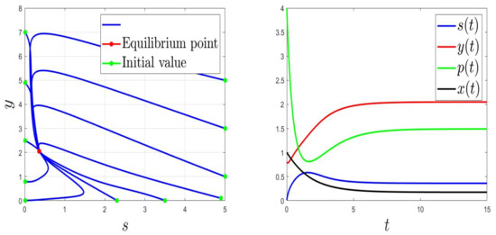
Figure 1.
Behaviours for and , then .
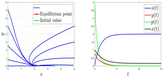
Figure 2.
Behaviours for and , then .
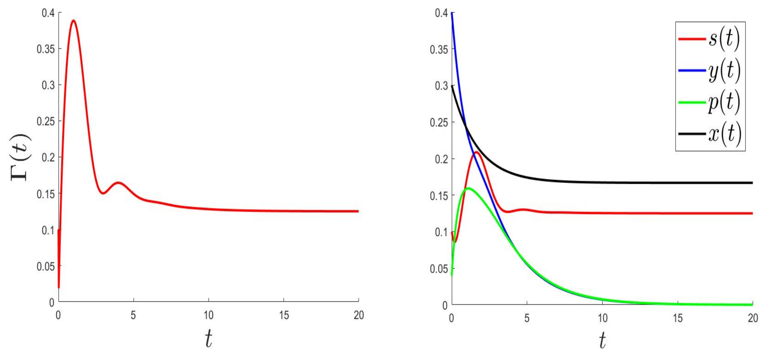
5.2. Numerical Simulations for the Control Problem
For the numerical resolution of the optimal control problem, we applied an appropriated scheme based on a modified Gauss-Seidel-like finite-difference scheme (see Appendix A). The parameter values were the same as in Figure 1 (where the equilibrium is globally asymptotically stable) but with a variable, . Those values were: and . Here, is a variable such that , and .
In Figure 3, Figure 4 and Figure 5, the behaviours of (left), and (right) were plotted for several values of , , and . As expected, the number of uninfected cells increased and converged to 0; however, the number of infected cells decreased. Figure 3, Figure 4 and Figure 5 (right) can be compared to Figure 3 in [5], giving the CHIKV pathogenesis.
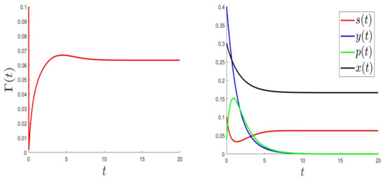
Figure 3.
.

Figure 4.
.
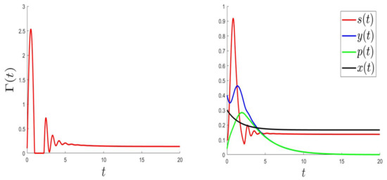
Figure 5.
.
6. Conclusions
In the present work, we considered and analyzed a mathematical system of differential equations modelling the Chikungunya virus (CHIKV) dynamics by two ways of infection and general incidence rates. The steady-states, which are the CHIKV-free equilibrium point and CHIKV endemic point, were determined and their local and global stability were studied, based on the basic reproduction number () obtained by the next-generation matrix. From the analysis, it was found that the disease-free point is locally asymptotically stable if , and the CHIKV endemic point is locally asymptotically stable if . The global stability of the equilibrium points were carried out using Lyapunov stability, and we confirmed the local stability results. These results are consistent with those obtained when using particular incidence rates as in [18]. We improved and developed the main mathematical techniques used in the previous studies [15,16,17,18,19,20,21]. Furthermore, we obtained the same sharp threshold criteria for the local and global stability of both disease-free and endemic steady-states. Later, we applied an optimal recruitment strategy to minimize the number of infected cells. We thus designed a nonlinear optimal control problem. Some numerical simulations were conducted to visualize the analytical results obtained.
There is still a series of questions of great interest. Current scientific research about the dynamics of a virus infection is mainly focused on solving three major issues: the role of time-delay, the space-time spread of a virus outbreak that occurs in a specific region of the territory, and the role of intrinsic fluctuations.
In this context, we can seek to develop a mathematical model which improves the model presented here by considering three types of infected cells, namely, latently infected cells, short-lived productively infected cells, and long-lived productively infected cells. Such a model can be applied to human immunodeficiency virus (HIV) dynamics.
Author Contributions
Conceptualization, S.A. and S.W.; Methodology, S.A. and S.W.; Writing—original draft, S.A. and S.W.; Writing—review & editing, S.A. and S.W. All authors have read and agreed to the published version of the manuscript.
Funding
This research received no external funding.
Institutional Review Board Statement
Not applicable.
Informed Consent Statement
Not applicable.
Data Availability Statement
Not applicable.
Acknowledgments
The authors are thankful to the editor and anonymous referees for their valuable comments and suggestions.
Conflicts of Interest
The authors declare no conflict of interest.
Appendix A. Applied Numerical Scheme
Let subdivide the time interval as the following: . Let , and are the approximation of the variables , , and the control at time . , and are the values of the variables , , and the control at time . , and are the values of the variables , , and the control at time . The state system was resolved using Gauss-Seidel-like implicit finite-difference method. The adjoint system was resolved using a backward-difference scheme as the following:
Hence we applied the algorithm hereafter
| Algorithm 1 |
1: , , 2: for to do end |
References
- Kraemer, M.U.; Reiner, R.C.; Brady, O.J.; Messina, J.P.; Gilbert, M.; Pigott, D.M.; Yi, D.; Johnson, K.; Earl, L.; Marczak, L.B.; et al. Past and future spread of the arbovirus vectors Aedes aegypti and Aedes albopictus. Nat. Microbiol. 2019, 4, 854. [Google Scholar] [CrossRef]
- Massad, E.; Ma, S.; Burattini, M.N.; Tun, Y.; Coutinho, F.A.B.; Ang, L.W. The risk of chikungunya fever in a dengue-endemic area. J. Travel Med. 2008, 15, 147–155. [Google Scholar] [CrossRef]
- Sourisseau, M.; Schilte, C.; Casartelli, N.; Trouillet, C.; Guivel-Benhassine, F.; Rudnicka, D.; Sol-Foulon, N.; Le Roux, K.; Prevost, M.C.; Fsihi, H.; et al. Characterization of reemerging chikungunya virus. PLoS Pathog. 2007, 3, e89. [Google Scholar] [CrossRef]
- Ozden, S.; Huerre, M.; Riviere, J.P.; Coffey, L.L.; Afonso, P.V.; Mouly, V.; de Monredon, J.; Roger, J.C.; El Amrani, M.; Yvin, J.L.; et al. Human muscle satellite cells as targets of Chikungunya virus infection. PLoS ONE 2007, 2, e527. [Google Scholar] [CrossRef]
- Schwartz, O.; Albert, M. Biology and pathogenesis of chikungunya virus. Nat. Rev. Microbiol. 2010, 8, 491–500. [Google Scholar] [CrossRef]
- Alsahafi, S.; Woodcock, S. Mutual inhibition in presence of a virus in continuous culture. Math. Biosci. Eng. 2021, 18, 3258–3273. [Google Scholar] [CrossRef] [PubMed]
- Alsahafi, S.; Woodcock, S. Local Analysis for a Mutual Inhibition in Presence of Two Viruses in a Chemostat. Nonlinear Dyn. Syst. Theory 2021, 21, 337–359. [Google Scholar]
- Arora, R.; Kumar, D.; Jhamb, I.; Narang, A.K. Mathematical Modeling of Chikungunya Dynamics: Stability and Simulation. Cubo 2020, 22, 177–201. [Google Scholar] [CrossRef]
- Dumont, Y.; Chiroleu, F.; Domerg, C. On a temporal model for the Chikungunya disease: Modeling, theory and numerics. Math. Biosci. 2008, 213, 80–91. [Google Scholar] [CrossRef]
- El Hajji, M.; Chorfi, N.; Jleli, M. Mathematical modelling and analysis for a three-tiered microbial food web in a chemostat. Electron. J. Differ. Equ. 2017, 2017, 1–13. [Google Scholar]
- El Hajji, M.; Chorfi, N.; Jleli, M. Mathematical model for a membrane bioreactor process. Electron. J. Differ. Equ. 2015, 2015, 1–7. [Google Scholar]
- El Hajji, M. Boundedness and asymptotic stability of nonlinear Volterra integro-differential equations using Lyapunov functional. J. King Saud Univ. Sci. 2019, 31, 1516–1521. [Google Scholar] [CrossRef]
- Li, F.; Wang, J. Analysis of an HIV infection model with logistic target cell growth and cell-to-cell transmission. Chaos Solitons Fractals 2015, 81, 136–145. [Google Scholar] [CrossRef]
- Long, K.M.; Heise, M.T. Protective and Pathogenic Responses to Chikungunya Virus Infection. Curr. Trop. Med. Rep. 2015, 2, 13–21. [Google Scholar] [CrossRef] [PubMed]
- Elaiw, A.M.; Alade, T.O.; Alsulami, S.M. Analysis of latent CHIKV dynamics models with general incidence rate and time delays. J. Biol. Dyn. 2018, 12, 700–730. [Google Scholar] [CrossRef] [PubMed]
- Elaiw, A.M.; Alade, T.O.; Alsulami, S.M. Analysis of within-host CHIKV dynamics models with general incidence rate. Int. J. Biomath. 2018, 11, 1850062. [Google Scholar] [CrossRef]
- Elaiw, A.M.; Almalki, S.E.; Hobiny, A.D. Global dynamics of Chikungunya virus with two routes of infection. J. Comput. Anal. Appl. 2020, 28, 481–490. [Google Scholar]
- Elaiw, A.M.; Almalki, S.E.; Hobiny, A.D. Global dynamics of humoral immunity Chikungunya virus with two routes of infection and Holling type—II. J. Math. Computer Sci. 2019, 19, 65–73. [Google Scholar] [CrossRef]
- Elaiw, A.M.; Almalki, S.E.; Hobiny, A.D. Stability of CHIKV infection models with CHIKV-monocyte and infected-monocyte saturated incidences. AIP Adv. 2019, 9, 025308. [Google Scholar] [CrossRef] [Green Version]
- El Hajji, M. Modelling and optimal control for Chikungunya disease. Theory Biosci. 2021, 140, 27–44. [Google Scholar] [CrossRef]
- El Hajji, M.; Zaghdani, A.; Sayari, S. Mathematical analysis and optimal control for Chikungunya virus with two routes of infection with nonlinear incidence rate. Int. J. Biomath. 2021, 2150088. [Google Scholar] [CrossRef]
- Wang, Y.; Liu, X. Stability and Hopf bifurcation of a within-host chikungunya virus infection model with two delays. Math. Comput. Simul. 2017, 138, 31–48. [Google Scholar] [CrossRef]
- Lai, X.; Zou, X. Modeling cell-to-cell spread of HIV-1 with logistic target cell growth. J. Math. Anal. Appl. 2015, 426, 563–584. [Google Scholar] [CrossRef]
- Lai, X.; Zou, X. Modelling HIV-1 virus dynamics with both virus-to-cell infection and cell-to-cell transmission. SIAM J. Appl. Math. 2014, 74, 898–917. [Google Scholar] [CrossRef]
- Wang, J.; Lang, J.; Zou, X. Analysis of an age structured HIV infection model with virus-to-cell infection and cell-to-cell transmission. Nonlinear Anal. Real World Appl. 2017, 34, 75–96. [Google Scholar] [CrossRef]
- Hethcote, H.W. The mathematics of infectious disease. SIAM Rev. 2000, 42, 599–653. [Google Scholar] [CrossRef] [Green Version]
- Diekmann, O.; Heesterbeek, J.A.P. On the definition and the computation of the basic reproduction ratio R0 in models for infectious diseases in heterogeneous populations. J. Math. Biol. 1990, 28, 365–382. [Google Scholar] [CrossRef] [PubMed] [Green Version]
- Diekmann, O.; Heesterbeek, J.A.P.; Roberts, M.G. The construction of next-generation matrices for compartmental epidemic models. J. R. Soc. Interface 2010, 7, 873–885. [Google Scholar] [CrossRef] [PubMed] [Green Version]
- Van den Driessche, P.; Watmough, J. Reproduction Numbers and Sub-Threshold Endemic Equilibria for Compartmental Models of Disease Transmission. Math. Biosci. 2002, 180, 29–48. [Google Scholar] [CrossRef]
- LaSalle, J.P. The Stability of Dynamical Systems; SIAM: Philadelphia, PA, USA, 1976. [Google Scholar]
- El Hajji, M.; Sayari, S.; Zaghdani, A. Mathematical analysis of an “SIR” epidemic model in a continuous reactor-deterministic and probabilistic approaches. J. Korean Math. Soc. 2021, 58, 45–67. [Google Scholar]
- El Hajji, M. How can inter-specific interferences explain coexistence or confirm the competitive exclusion principle in a chemostat. Int. J. Biomath. 2018, 11, 1850111. [Google Scholar] [CrossRef]
- Fleming, W.H.; Rishel, R.W. Deterministic and Stochastic Optimal Control; Springer: New York, NY, USA, 1975. [Google Scholar]
- Lenhart, S.; Workman, J.T. Optimal Control Applied to Biological Models; Chapman and Hall: London, UK, 2007. [Google Scholar]
- Pontryagin, L.S.; Boltyanskii, V.G.; Gamkrelidze, R.V.; Mishchenko, E.F. The Mathematical Theory of Optimal Processes; Wiley: New York, NY, USA, 1962. [Google Scholar]


Publisher’s Note: MDPI stays neutral with regard to jurisdictional claims in published maps and institutional affiliations. |
© 2021 by the authors. Licensee MDPI, Basel, Switzerland. This article is an open access article distributed under the terms and conditions of the Creative Commons Attribution (CC BY) license (https://creativecommons.org/licenses/by/4.0/).