Article

A Novel Technique to Control the Accuracy of a Nonlinear Fractional Order Model of COVID-19: Application of the CESTAC Method and the CADNA Library

1
Industrial Mathematics Laboratory, Baikal School of BRICS, Irkutsk National Research Technical University, 664074 Irkutsk, Russia
2
Department of Applied Mathematics and Programming, South Ural State University, Lenin Prospect 76, 454080 Chelyabinsk, Russia
3
Department of Mathematics and Computer Science, Babeş-Bolyai University, 400084 Cluj-Napoca, Romania
4
Instituto de Matemáticas, Departamento de Estatística, Análise Matemática e Optimización, Universidade de Santiago de Compostela, 15782 Santiago de Compostela, Spain
*
Author to whom correspondence should be addressed.
Mathematics 2021, 9(12), 1321; https://doi.org/10.3390/math9121321
Submission received: 1 May 2021 / Revised: 31 May 2021 / Accepted: 7 June 2021 / Published: 8 June 2021
(This article belongs to the Special Issue Mathematical Modeling and Analysis in Biology and Medicine)

Abstract

:
In this paper, a nonlinear fractional order model of COVID-19 is approximated. For this aim, at first we apply the Caputo–Fabrizio fractional derivative to model the usual form of the phenomenon. In order to show the existence of a solution, the Banach fixed point theorem and the Picard–Lindelof approach are used. Additionally, the stability analysis is discussed using the fixed point theorem. The model is approximated based on Indian data and using the homotopy analysis transform method (HATM), which is among the most famous, flexible and applicable semi-analytical methods. After that, the CESTAC (Controle et Estimation Stochastique des Arrondis de Calculs) method and the CADNA (Control of Accuracy and Debugging for Numerical Applications) library, which are based on discrete stochastic arithmetic (DSA), are applied to validate the numerical results of the HATM. Additionally, the stopping condition in the numerical algorithm is based on two successive approximations and the main theorem of the CESTAC method can aid us analytically to apply the new terminations criterion instead of the usual absolute error that we use in the floating-point arithmetic (FPA). Finding the optimal approximations and the optimal iteration of the HATM to solve the nonlinear fractional order model of COVID-19 are the main novelties of this study.

1. Introduction

Corona virus infection (COVID-19) is an infectious disease caused by the newly discovered Corona virus. Most people with COVID-19 disease experience mild to moderate symptoms and recover without special treatment. The virus that causes COVID-19 is mainly transmitted through particles produced when a person coughs, sneezes, or exhales. These particles do not stay suspended in the air due to their weight and fall quickly on the ground or surfaces. If you are close to a person with COVID-19, you may become infected by inhaling the virus or touching the infected surface and then touching your eyes, nose, or mouth. According to WHO reports until 2 March 2021, more than 115 million infected, more than 2.5 million dead and more than 90 million recovered people from more than 200 countries have been identified [1].
Thus, providing mathematical models to control and predict the behavior of this pandemic is urgent [2]. Recently, many mathematical models related to COVID-19 have been studied [3,4]. In [5], an analysis model of diagnosis and treatment for the COVID-19 pandemic based on medical information fusion was discussed, in [6] a model of the COVID-19 epidemic and predicting its future situation in Ethiopia was studied and in [7] a fractional order COVID-19 model with real-life data application was analyzed. The COVID-19 epidemic and clinical risk factors of patients under an epidemiological Markov model were discussed in [8] and the incorporating social determinants of health into modeling of COVID-19 and other infectious diseases was illustrated in [9].
Recently, due to their importance and more accurate results, fractional order models are among the most studied problems in the world. In [10], the authors focused on a Caputo–Fabrizio fractional model of COVID-19. In [11], a fractional order model of HIV infection was discussed, in [12] the application of the Atangana–Baleanu fractional derivative in mathematical biology was studied and in [13], a fractional order HIV model with Caputo and constant proportional Caputo operators was illustrated. An application of the Caputo–Fabrizio fractional derivative to solve a fractional order model of an energy supply–demand system can be found in [14]. For other applications of the fractional order models and also their usual forms please see [15,16,17,18,19,20].
The homotopy analysis method (HAM) presented by Liao [21,22,23] is one of the most flexible and accurate methods for solving various linear and nonlinear problems. This method has been applied for solving many problems, such as solving integral equations [24,25], solving singular problems [26,27] and a modified non-linear epidemiological model of computer viruses [28].
We should note that all of the mentioned researches are based on the FPA, and in order to show the accuracy of the methods, we apply the traditional absolute error or residual error in the form of
| g ( x ) g m ( x ) | < ε , o r | g m ( x ) g m 1 ( x ) | < ε ,
where the exact and approximate solutions are denoted by g ( x ) and g m ( x ) , respectively and ε is a small positive value. Thus, in order to apply Condition (1), not only should we know the exact solution g ( x ) but we should also have the optimal value of ε , which are disadvantages of methods based on the FPA. Concerning ε , for small values we will have extra iterations without improving the accuracy of the results and for large values we will have only one or two iterations without providing accurate results. Thus, we apply the CESTAC method and the CADNA library, which are based on the DSA. This method was presented by Laporte and Vignes [29] for the first time and after that other researchers improved the method and library [30]. Using this method we do not need to have the exact solutions and ε and the termination criterion will be in the following form:
| g m ( x ) g m 1 ( x ) | = @ . 0 ,
where g m ( x ) and g m 1 ( x ) are two successive approximations and @ . 0 denotes the informatical zero. Applying Condition (2), we do not need to have the exact solution and it is important that it does not depend on a positive small value such as ε . Additionally, in this method, instead of applying the usual softwares, we apply the CADNA library. This library should be applied on a Linux operating system and all codes should be written using C, C++, FORTRAN or ADA codes [31,32,33]. The informatical zero sign can be produced only using the DSA and the CADNA library. This shows that the number of common significant digits for two successive approximations are almost equal to the number of common significant digits of the exact and approximate solutions [33,34,35]. Thus, we will be able to apply Condition (2) instead of (1). Recently, we focused on validating the numerical results of various problems using the CESTAC method. In [36], the results of the Adomian decomposition method for solving Volterra integral equation with a discontinuous kernel was studied and in [37,38] the CESTAC method was used to validate the results on the reverse osmosis system. Dynamical control on the homotopy perturbation method and the Taylor-collocation method to solve Volterra integral equations with piecewise smooth kernels was discussed in [39,40]. In [41], we illustrated the Sinc-collocation method for solving various kinds of crisp and fuzzy integral equations and finally, we applied the CADNA library to control the accuracy of the load leveling problem in [42].
In this paper, a nonlinear fractional order model of COVID-19 will be discussed based on the Caputo–Fabrizio fractional derivative. The Picard–Lindelof approach and the Banach fixed point theorem are used to show the existence of the solution of the model. Additionally, the stability of the model is illustrated applying the fixed point theorem. The HATM is applied to solve the model and the numerical results are validated applying the CESTAC method and the CADNA library. Additionally, the main theorem of the CESTAC method is proven, which guarantees the accuracy of the numerical results obtained using Condition (2) instead of (1). Using this method, the optimal approximations and the optimal iteration to solve the model using the HATM are obtained, which are the main novelties of this study.

2. Preliminaries

In this section, we present some definitions and details of fractional derivatives [43,44].
Definition 1
([43]). Let g C n . The ω-th order Caputo fractional derivative can be defined via integrable differentiations as follows:
C D ω g ( t ) = 1 Γ ( n ω ) 0 t g ( n ) ( s ) ( t s ) ω n + 1 d s , n = [ ω ] + 1 ,
where g ( n ) L 1 .
Definition 2
([43]). The ω-th order Caputo–Fabrizio derivative for b > a , g H 1 ( a , b ) , and ω ( 0 , 1 ) is defined in the following form:
C F D ω g ( t ) = M ( ω ) 1 ω a t e x p ω 1 ω ( t s ) g ( s ) d s , t 0 ,
where M ( ω ) depending on ω denotes a normalization function and M ( 0 ) = M ( 1 ) = 1 . For a function g that is not in H 1 ( a , b ) , this derivative can be presented for g L 1 ( , b ) as follows:
C F D ω g ( t ) = ω M ( ω ) 1 ω b ( g ( t ) g ( s ) ) e x p ( ω 1 ω ( t s ) ) d s , 0 < ω < 1 .
In addition, the ω + n -th order fractional derivative C F D ω + n for n 1 and ω ( 0 , 1 ) can be defined as C F D ω + n g ( t ) : = C F D ω ( D n g ( t ) ) .
Definition 3
([44]). For 0 < ω 1 and M ( ω ) = 1 , the Laplace transform for the Caputo–Fabrizio derivative can be presented in the following form:
L [ C F D ω + n g ( t ) ] ( s ) = s n + 1 L [ g ( t ) ] s n g ( 0 ) s n 1 g ( 0 ) f ( n ) ( 0 ) s + ω ( 1 s ) .
Definition 4
([44]). The ω-order Riemann–Liouville fractional integral for R e ( ω ) > 0 is specified as:
I ω g ( t ) = 1 Γ ( ω ) 0 t ( t s ) ω 1 g ( s ) d s .
Definition 5
([44]). The fractional integral of Caputo–Fabrizio is defined by
C F I ω g ( t ) = 2 ( 1 ω ) ( 2 ω ) M ( ω ) g ( t ) + 2 ( ω ) ( 2 ω ) M ( ω ) 0 t g ( s ) d s , 0 < ω < 1 .
Additionally, the left and right fractional integrals of ( a C F D ω ) are defined [45] respectively by:
( C F I a ω g ) ( t ) = 1 ω B ( ω ) g ( t ) + ω B ( ω ) a t g ( s ) d s , ( C F I b ω g ) ( t ) = 1 ω B ( ω ) g ( t ) + ω B ( ω ) t b g ( s ) d s .
We have the following definitions for the Sumudu transform, x which is based on the classical Fourier integral [46,47,48].
Definition 6
([47]). Let A = { G : λ , k 1 , k 2 0 , | G ( t ) | < λ e x p ( t k j ) , t ( 1 ) j × [ 0 , ) } . Then S T [ g ( t ) ; u ] = G ( u ) denotes the Sumudu transform of a function g ( t ) A that is defined as
G ( u ) = S T [ g ( t ) ; u ] = 1 u 0 e x p ( t / u ) g ( t ) d t , u ( k 1 , k 2 ) ,
for all t 0 . Additionally, g ( t ) = S T 1 [ G ( u ) ] is the inverse Sumudu transform of G ( u ) .
Definition 7
([46]). For ( m 1 < ω m ) we can define the Sumudu transform for the Caputo derivative as
S T [ c D t ω g ( t ) ; u ] = u ω G ( u ) i = 0 m u ω i [ c D ω i g ( t ) ] t = 0 .
Definition 8
([49]). Assume that G is a function and it has a Caputo–Fabrizio fractional derivative. We can define the Sumudu transform of G with the Caputo–Fabrizio fractional derivative as
S T ( 0 C F D t ω ) ( G ( t ) ) = M ( ω ) 1 ω + ω u [ S T ( G ( t ) ) G ( 0 ) ] .
Definition 9.
[50] For a metric space ( X , d ) , a map g : X X is called a Picard operator whenever there exists x * X such that F i x ( g ) = { x * } and the sequence ( g n ( x 0 ) ) n N converges to x * for all x 0 X .
Definition 10.
Consider the Banach space ( Y , . ) , a self-map G on Y, and the recursive relation P n + 1 = ϕ ( G , P n ) . Let Ω ( G ) be the fixed point set of G, which includes Ω ( G ) and lim n P n = p Ω ( G ) . Suppose that { g n } Ω and e n = g n + 1 ϕ ( G , g n ) , if lim n e n = 0 implies that lim n g n = p , then the recursive procedure P n + 1 = ϕ ( G , P n ) is G-stable. Suppose that our sequence g n has an upper boundary. If Picard’s iteration P n + 1 = G P n is satisfied in all these conditions, then P n + 1 = G P n is G-stable.
Theorem 1
([50]). Assume that ( Y , . ) is a Banach space and G is a self-map of Y such that
G x G y R x G x + r x y ,
for all x , y Y , where R 0 and 0 r < 1 . Then G is Picard G-stable.

3. Nonlinear Fractional Order Model of COVID-19

Consider the following non-linear bio-mathematical model [51,52]:
d S d t = β I S , d E d t = β I S ε E , d I d t = ε E γ I d I q I , d Q d t = q I q t Q d Q , d R d t = γ I + q t Q , d D d t = d I + d Q ,
where S , E , I , Q , R and D are susceptible, exposed, infected, quarantined, recovered and dead populations, respectively, and we denote by N = S + E + I + Q + R + D the total size of the population. Susceptible individuals become infected at a rate, β , by infectious individuals, and the rate can be obtained using β = R 0 γ where R 0 is the basic reproduction number and γ = 1 i n f e c t i o u s p e r i o d . ε = 1 i n c u b a t i o n p e r i o d . We should note that D is a fraction of I + Q . The death rate is denoted by d, the fraction of active cases quarantined is denoted by q and the time period of quarantine is indicated by q t . The graphical form of the model is shown in Figure 1 [51]. The values and parameters of this model are presented in Table 1, based on Indian data [51].
Model (3) can be written using the ω -th order Caputo–Fabrizio fractional derivative as follows:
0 C F D t ω S = β I S , 0 C F D t ω E = β I S ε E , 0 C F D t ω I = ε E γ I d I q I , 0 C F D t ω Q = q I q t Q d Q , 0 C F D t ω R = γ I + q t Q , 0 C F D t ω D = d I + d Q .

4. Existence of Solution

Applying Definition 5 to both sides of Equation (4), we obtain:
S ( t ) u 1 ( t ) = 2 ( 1 ω ) ( 2 ω ) M ( ω ) { β I ( t ) S ( t ) } + 2 ω ( 2 ω ) M ( ω ) 0 t [ β I ( s ) S ( s ) ] d s , E ( t ) u 2 ( t ) = 2 ( 1 ω ) ( 2 ω ) M ( ω ) { β I ( t ) S ( t ) ε E ( t ) } + 2 ω ( 2 ω ) M ( ω ) 0 t [ β I ( s ) S ( s ) ε E ( s ) ] d s , I ( t ) u 3 ( t ) = 2 ( 1 ω ) ( 2 ω ) M ( ω ) { ε E ( t ) γ I ( t ) d I ( t ) q I ( t ) } + 2 ω ( 2 ω ) M ( ω ) 0 t [ ε E ( s ) γ I ( s ) d I ( s ) q I ( s ) ] d s , Q ( t ) u 4 ( t ) = 2 ( 1 ω ) ( 2 ω ) M ( ω ) { q I ( t ) q t Q ( t ) d Q ( t ) } + 2 ω ( 2 ω ) M ( ω ) 0 t [ q I ( s ) q t Q ( s ) d Q ( s ) ] d s , R ( t ) u 5 ( t ) = 2 ( 1 ω ) ( 2 ω ) M ( ω ) { γ I ( t ) + q t Q ( t ) } + 2 ω ( 2 ω ) M ( ω ) 0 t [ γ I ( s ) + q t Q ( s ) ] d s , D ( t ) u 6 ( t ) = 2 ( 1 ω ) ( 2 ω ) M ( ω ) { d I ( t ) + d Q ( t ) } + 2 ω ( 2 ω ) M ( ω ) 0 t [ d I ( s ) + d Q ( s ) ] d s .
By assuming S 0 ( t ) = u 1 ( t ) , E 0 ( t ) = u 2 ( t ) , I 0 ( t ) = u 3 ( t ) , Q 0 ( t ) = u 4 ( t ) , R 0 ( t ) = u 5 ( t ) and D 0 ( t ) = u 6 ( t ) , these equations can be written in the following form:
S n + 1 ( t ) = 2 ( 1 ω ) ( 2 ω ) M ( ω ) { β I n ( t ) S n ( t ) } + 2 ω ( 2 ω ) M ( ω ) 0 t [ β I n ( s ) S n ( s ) ] d s , E n + 1 ( t ) = 2 ( 1 ω ) ( 2 ω ) M ( ω ) { β I n ( t ) S n ( t ) ε E n ( t ) } + 2 ω ( 2 ω ) M ( ω ) 0 t [ β I n ( s ) S n ( s ) ε E n ( s ) ] d s , I n + 1 ( t ) = 2 ( 1 ω ) ( 2 ω ) M ( ω ) { ε E n ( t ) γ I n ( t ) d I n ( t ) q I n ( t ) } + 2 ω ( 2 ω ) M ( ω ) 0 t [ ε E n ( s ) γ I n ( s ) d I n ( s ) q I n ( s ) ] d s , Q n + 1 ( t ) = 2 ( 1 ω ) ( 2 ω ) M ( ω ) { q I n ( t ) q t Q n ( t ) d Q n ( t ) } + 2 ω ( 2 ω ) M ( ω ) 0 t [ q I n ( s ) q t Q n ( s ) d Q n ( s ) ] d s , R n + 1 ( t ) = 2 ( 1 ω ) ( 2 ω ) M ( ω ) { γ I n ( t ) + q t Q n ( t ) } + 2 ω ( 2 ω ) M ( ω ) 0 t [ γ I n ( s ) + q t Q n ( s ) ] d s , D n + 1 ( t ) = 2 ( 1 ω ) ( 2 ω ) M ( ω ) { d I n ( t ) + d Q n ( t ) } + 2 ω ( 2 ω ) M ( ω ) 0 t [ d I n ( s ) + d Q n ( s ) ] d s ,
and by letting n approach infinity in Equation (6), the approximate solutions can be obtained as:
lim n S n ( t ) = S ( t ) , lim n Q n ( t ) = Q ( t ) , lim n E n ( t ) = E ( t ) , lim n R n ( t ) = R ( t ) , lim n I n ( t ) = I ( t ) , lim n D n ( t ) = D ( t ) .
Now we can apply the Picard–Lindelof approach and the Banach fixed point theorem to show the existence of a solution to Equation (4). First we define the following operators as:
u 1 ( t , S ) = β I S , u 2 ( t , E ) = β I S ε E , u 3 ( t , I ) = ε E γ I d I q I , u 4 ( t , Q ) = q I q t Q d Q , u 5 ( t , R ) = γ I + q t Q , u 6 ( t , D ) = d I + d Q .
Let
1 = sup C [ a , ρ 1 ] u 1 ( t , S ) , 2 = sup C [ a , ρ 2 ] u 2 ( t , E ) , 3 = sup C [ a , ρ 3 ] u 3 ( t , I ) , 4 = sup C [ a , ρ 4 ] u 4 ( t , Q ) , 5 = sup C [ a , ρ 5 ] u 5 ( t , R ) , 6 = sup C [ a , ρ 6 ] u 6 ( t , D ) ,
where
C [ a , ρ 1 ] = | t a , t + a | × | S ρ 1 , S + ρ 1 | = B × C 1 , C [ a , ρ 2 ] = | t a , t + a | × | E ρ 2 , E + ρ 2 | = B × C 2 , C [ a , ρ 3 ] = | t a , t + a | × | I ρ 3 , I + ρ 3 | = B × C 3 , C [ a , ρ 4 ] = | t a , t + a | × | Q ρ 4 , Q + ρ 4 | = B × C 4 , C [ a , ρ 5 ] = | t a , t + a | × | R ρ 5 , R + ρ 5 | = B × C 5 , C [ a , ρ 6 ] = | t a , t + a | × | D ρ 6 , D + ρ 6 | = B × C 6 .
Assuming a uniform norm
Z ( t ) = sup t [ t a , t + a ] | Z ( t ) | ,
on C [ a , ρ i ] , i = 1 , , 5 , and defining the Picard operator as
O : C ( B , C 1 , , C 6 ) C ( B , C 1 , , C 6 ) ,
we can write
O ( Z ( t ) ) = Z 0 ( t ) + 2 ( 1 ω ) ( 2 ω ) M ( ω ) G ( t , Z ( t ) ) + 2 ω ( 2 ω ) M ( ω ) 0 t G ( s , Z ( s ) ) d s ,
where Z ( t ) = { S ( t ) , E ( t ) , I ( t ) , Q ( t ) , R ( t ) , D ( t ) } and Z 0 ( t ) = { S ( 0 ) , E ( 0 ) , I ( 0 ) , Q ( 0 ) , R ( 0 ) , D ( 0 ) } and
G ( t , Z ( t ) ) = { u 1 ( t , S ) , u 2 ( t , E ) , u 3 ( t , I ) , u 4 ( t , Q ) , u 5 ( t , R ) , u 6 ( t , D ) } ,
and thus
Z ( t ) max { ρ 1 , , ρ 6 } = C .
Assume that L = max { L 1 , , L 6 } and there is t 0 such that t 0 t and
O ( Z ( t ) ) Z 0 ( t ) = 2 ( 1 ω ) ( 2 ω ) M ( ω ) G ( t , Z ( t ) ) + 2 ω ( 2 v ) M ( v ) 0 t G ( s , Z ( s ) ) d s 2 ( 1 ω ) ( 2 ω ) M ( ω ) G ( t , Z ( t ) ) + 2 ω ( 2 ω ) M ( ω ) 0 t G ( s , Z ( s ) ) d s 2 ( 1 ω ) ( 2 ω ) M ( ω ) + 2 ω t ( 2 ω ) M ( ω ) L
2 ( 1 ω ) ( 2 ω ) M ( ω ) + 2 ω t 0 ( 2 v ) M ( v ) L μ L C ,
where
μ < C L .
Now, we can write
O Z 1 O Z 2 = sup t B | Z 1 ( t ) Z 2 ( t ) | ,
and using definition of the Picard operator we obtain
O Z 1 O Z 2 = 2 ( 1 ω ) ( 2 ω ) M ( ω ) { G ( t , Z 1 ( t ) ) G ( t , Z 2 ( t ) ) } + 2 ω ( 2 ω ) M ( ω ) 0 t { G ( s , Z 1 ( s ) ) G ( s , Z 2 ( s ) ) } d s 2 ( 1 ω ) ( 2 ω ) M ( ω ) G ( t , Z 1 ( t ) ) G ( t , Z 2 ( t ) ) + 2 ω ( 2 ω ) M ( ω ) 0 t G ( s , Z 1 ( s ) ) G ( s , Z 2 ( s ) ) d s 2 ( 1 ω ) ( 2 ω ) M ( ω ) λ Z 1 ( t ) Z 2 ( t ) + 2 ω λ ( 2 ω ) M ( ω ) 0 t Z 1 ( s ) Z 2 ( s ) d s 2 ( 1 ω ) λ ( 2 ω ) M ( ω ) + 2 ω λ t 0 ( 2 ω ) M ( ω ) Z 1 ( t ) Z 2 ( t ) μ λ Z 1 ( t ) Z 2 ( t ) ,
where λ < 1 . We know that G is a contraction so μ λ < 1 and O is a contraction, showing that the proof is complete.

5. Special Solution via Iteration Approach

In this section, using the Sumudu transform, we can provide a special solution. Applying this transformation on both sides of (4) we obtain:
S T ( 0 C F D t ω S ( t ) ) = S T ( β I ( t ) S ( t ) ) , S T ( 0 C F D t ω E ( t ) ) = S T ( β I ( t ) S ( t ) ε E ( t ) ) , S T ( 0 C F D t ω I ( t ) ) = S T ( ε E ( t ) γ I ( t ) d I ( t ) q I ( t ) ) , S T ( 0 C F D t ω Q ( t ) ) = S T ( q I ( t ) q t Q ( t ) d Q ( t ) ) , S T ( 0 C F D t ω R ( t ) ) = S T ( γ I ( t ) + q t Q ( t ) ) , S T ( 0 C F D t ω D ( t ) ) = S T ( d I ( t ) + d Q ( t ) ) ,
and based on the definition of the Sumudu transform we can write
M ( ω ) 1 ω + ω u ( S T ( S ( t ) ) S ( 0 ) ) = S T ( β I ( t ) S ( t ) ) , M ( ω ) 1 ω + ω u ( S T ( E ( t ) ) E ( 0 ) ) = S T ( β I ( t ) S ( t ) ε E ( t ) ) , M ( ω ) 1 ω + ω u ( S T ( I ( t ) ) I ( 0 ) ) = S T ( ε E ( t ) γ I ( t ) d I ( t ) q I ( t ) ) , M ( ω ) 1 ω + ω u ( S T ( Q ( t ) ) Q ( 0 ) ) = S T ( q I ( t ) q t Q ( t ) d Q ( t ) ) , M ( ω ) 1 ω + ω u ( S T ( R ( t ) ) R ( 0 ) ) = S T ( γ I ( t ) + q t Q ( t ) ) , M ( ω ) 1 ω + ω u ( S T ( D ( t ) ) D ( 0 ) ) = S T ( d I ( t ) + d Q ( t ) ) ,
and
S T ( S ( t ) ) = S ( 0 ) + 1 ω + ω u M ( ω ) S T ( β I ( t ) S ( t ) ) , S T ( E ( t ) ) = E ( 0 ) + 1 ω + ω u M ( ω ) S T ( β I ( t ) S ( t ) ε E ( t ) ) , S T ( I ( t ) ) = I ( 0 ) + 1 ω + ω u M ( ω ) S T ( ε E ( t ) γ I ( t ) d I ( t ) q I ( t ) ) , S T ( Q ( t ) ) = Q ( 0 ) + 1 ω + ω u M ( ω ) S T ( q I ( t ) q t Q ( t ) d Q ( t ) ) , S T ( R ( t ) ) = R ( 0 ) + 1 ω + ω u M ( ω ) S T ( γ I ( t ) + q t Q ( t ) ) , S T ( D ( t ) ) = D ( 0 ) + 1 ω + ω u M ( ω ) S T ( d I ( t ) + d Q ( t ) ) .
Finally, the following recursive relation can be obtained as
S n + 1 ( t ) = S n ( t ) + S T 1 1 ω + ω u M ( ω ) S T ( β I n ( t ) S n ( t ) ) , E n + 1 ( t ) = E n ( t ) + S T 1 1 ω + ω u M ( ω ) S T ( β I n ( t ) S n ( t ) ε E n ( t ) ) , I n + 1 ( t ) = I n ( t ) + S T 1 1 ω + ω u M ( ω ) S T ( ε E n ( t ) γ I n ( t ) d I n ( t ) q I n ( t ) ) , Q n + 1 ( t ) ) = Q n ( t ) + S T 1 1 ω + ω u M ( ω ) S T ( q I n ( t ) q t Q n ( t ) d Q n ( t ) ) , R n + 1 ( t ) = R n ( t ) + S T 1 1 ω + ω u M ( ω ) S T ( γ I n ( t ) + q t Q n ( t ) ) , D n + 1 ( t ) = D n ( t ) + S T 1 1 ω + ω u M ( ω ) S T ( d I n ( t ) + d Q n ( t ) ) ,
where the approximate solutions can be found using the following relations
lim n S n ( t ) = S ( t ) , lim n E n ( t ) = E ( t ) , lim n I n ( t ) = I ( t ) , lim n Q n ( t ) = Q ( t ) , lim n R n ( t ) = R ( t ) , lim n D n ( t ) = D ( t ) .

Fixed Point Theorem for Stability Analysis of the Iteration Method

Theorem 2.
Let F be a self-map that is defined in the following form: -5.0cm0cm
F ( S n ( t ) ) = S n + 1 ( t ) = S n ( t ) + S T 1 1 ω + ω u M ( ω ) S T ( β I n ( t ) S n ( t ) ) , F ( E n ( t ) ) = E n + 1 ( t ) = E n ( t ) + S T 1 1 ω + ω u M ( ω ) S T ( β I n ( t ) S n ( t ) ε E n ( t ) ) , F ( I n ( t ) ) = I n + 1 ( t ) = I n ( t ) + S T 1 1 ω + ω u M ( ω ) S T ( ε E n ( t ) γ I n ( t ) d I n ( t ) q I n ( t ) ) , F ( Q n ( t ) ) = Q n + 1 ( t ) ) = Q n ( t ) + S T 1 1 ω + ω u M ( ω ) S T ( q I n ( t ) q t Q n ( t ) d Q n ( t ) ) , F ( R n ( t ) ) = R n + 1 ( t ) = R n ( t ) + S T 1 1 ω + ω u M ( ω ) S T ( γ I n ( t ) + q t Q n ( t ) ) , F ( D n ( t ) ) = D n + 1 ( t ) = D n ( t ) + S T 1 1 ω + ω u M ( ω ) S T ( d I n ( t ) + d Q n ( t ) ) .
Formula (26) is F-stable in L 1 ( a , b ) if
1 β P 3 k 1 ( η ) β P 1 k 2 ( η ) < 1 , 1 + β P 3 k 3 ( η ) β P 1 k 4 ( η ) ε k 5 ( η ) < 1 , 1 + ε k 6 ( η ) ( γ + d + q ) k 7 ( η ) < 1 , 1 + q k 8 ( η ) ( q t + d ) k 9 ( η ) < 1 , 1 + γ k 10 ( η ) + q t k 11 ( η ) < 1 , 1 + d k 12 ( η ) + d k 13 ( η ) < 1 .
Proof. 
In order to prove the theorem, first the following relation should be computed for ( n , m ) N × N to show that F has a fixed point as
F ( S n ( t ) ) F ( S m ( t ) ) = S n ( t ) S m ( t ) + S T 1 1 ω + ω u M ( ω ) S T ( β I n ( t ) S n ( t ) ) S T 1 1 ω + ω u M ( ω ) S T ( β I m ( t ) S m ( t ) ) ,
and taking the norm on both sides of Equation (28) we obtain:
F ( S n ) F ( S m ) = S n S m + S T 1 1 ω + ω u M ( ω ) S T ( β ( I n S n I m S m ) ) , S n S m + S T 1 1 ω + ω u M ( ω ) S T ( β I n ( S n S m ) + β S m ( I n I m ) ) .
Because of the same role of both solutions, we obtain:
S n ( t ) S m ( t ) E n ( t ) E m ( t ) I n ( t ) I m ( t ) Q n ( t ) Q m ( t ) R n ( t ) R m ( t ) D n ( t ) D m ( t ) ,
and applying (29) and (30) we can write -4.6cm0cm
F ( S n ( t ) ) F ( S m ( t ) ) S n ( t ) S m ( t ) + S T 1 1 ω + ω u M ( ω ) S T ( β I n ( t ) ( S n ( t ) S m ( t ) ) + β S m ( t ) ( S n ( t ) S m ( t ) ) ) .
We know that S n , E n , I n , Q n , R n , D n are bounded because they are convergent sequences. Thus for all t, there are values P 1 , P 2 , P 3 , P 4 , P 5 , P 6 such that
S m < P 1 , E n < P 2 , I n < P 3 , Q n < P 4 , R n < P 5 , D n < P 6 ,
where ( m , n ) N × N . Now, based on Equations (31) and (32) we obtain:
F ( S n ) F ( S m ) 1 β P 3 k 1 ( η ) β P 1 k 2 ( η ) S n S m ,
where k i are obtained from S T 1 1 ω + ω u M ( ω ) S T . . By repeating the process we have
F ( E n ) F ( E m ) 1 + β P 3 k 3 ( η ) β P 1 k 4 ( η ) ε k 5 ( η ) E n E m , F ( I n ) F ( I m ) 1 + ε k 6 ( η ) ( γ + d + q ) k 7 ( η ) I n I m , F ( Q n ) F ( Q m ) 1 + q k 8 ( η ) ( q t + d ) k 9 ( η ) Q n Q m , F ( R n ) F ( R m ) 1 + γ k 10 ( η ) + q t k 11 ( η ) R n R m , F ( D n ) F ( D m ) 1 + d k 12 ( η ) + d k 13 ( η ) D n D m ,
where
1 β P 3 k 1 ( η ) β P 1 k 2 ( η ) < 1 , 1 + β P 3 k 3 ( η ) β P 1 k 4 ( η ) ε k 5 ( η ) < 1 , 1 + ε k 6 ( η ) ( γ + d + q ) k 7 ( η ) < 1 , 1 + q k 8 ( η ) ( q t + d ) k 9 ( η ) < 1 , 1 + γ k 10 ( η ) + q t k 11 ( η ) < 1 , 1 + d k 12 ( η ) + d k 13 ( η ) < 1 .
Then, the F self-mapping has a fixed point. In addition, we show that F satisfies the conditions in Theorem 1. By assuming that (33) and (34) hold, we have R = ( 0 , 0 , 0 , 0 , 0 ) and
r = 1 β P 3 k 1 ( η ) β P 1 k 2 ( η ) , 1 + β P 3 k 3 ( η ) β P 1 k 4 ( η ) ε k 5 ( η ) , 1 + ε k 6 ( η ) ( γ + d + q ) k 7 ( η ) , 1 + q k 8 ( η ) ( q t + d ) k 9 ( η ) , 1 + γ k 10 ( η ) + q t k 11 ( η ) , 1 + d k 12 ( η ) + d k 13 ( η ) .
Then the conditions of Theorem 1 are satisfied and the proof is concluded.

6. Application of the HATM to Solve the Model

In order to apply the HATM for solving the fractional order model (4), applying the Laplace transformation we obtain:
L [ 0 C F D t ω S ] = L [ β I S ] , L [ 0 C F D t ω E ] = L [ β I S ε E ] , L [ 0 C F D t ω I ] = L [ ε E γ I d I q I ] , L [ 0 C F D t ω Q ] = L [ q I q t Q d Q ] , L [ 0 C F D t ω R ] = L [ γ I + q t Q ] , L [ 0 C F D t ω D ] = L [ d I + d Q ] .
Additionally, we can write
s L ( S ) S ( 0 ) s + ω ( 1 s ) = L [ β I S ] , s L ( E ) E ( 0 ) s + ω ( 1 s ) = L [ β I S ε E ] , s L ( I ) I ( 0 ) s + ω ( 1 s ) = L [ ε E γ I d I q I ] , s L ( Q ) Q ( 0 ) s + ω ( 1 s ) = L [ q I q t Q d Q ] , s L ( R ) R ( 0 ) s + ω ( 1 s ) = L [ γ I + q t Q ] , s L ( D ) D ( 0 ) s + ω ( 1 s ) = L [ d I + d Q ] ,
and we have
L ( S ) S 0 s s + ω ( 1 s ) s L [ β I S ] = 0 , L ( E ) E 0 s s + ω ( 1 s ) s L [ β I S ε E ] = 0 , L ( I ) I 0 s s + ω ( 1 s ) s L [ ε E γ I d I q I ] = 0 , L ( Q ) Q 0 s s + ω ( 1 s ) s L [ q I q t Q d Q ] = 0 , L ( R ) R 0 s s + ω ( 1 s ) s L [ γ I + q t Q ] = 0 , L ( D ) D 0 s s + ω ( 1 s ) s L [ d I + d Q ] = 0 .
We define the nonlinear operators as follows:
N 1 ( φ 1 ( t ; p ) , , φ 6 ( t ; p ) ) = L ( S ) S 0 s s + ω ( 1 s ) s L [ β φ 3 ( t ; p ) φ 1 ( t ; p ) ] , N 2 ( φ 1 ( t ; p ) , , φ 6 ( t ; p ) ) = L ( E ) E 0 s s + ω ( 1 s ) s L [ β φ 3 ( t ; p ) φ 1 ( t ; p ) ε φ 2 ( t ; p ) ] , N 3 ( φ 1 ( t ; p ) , , φ 6 ( t ; p ) ) = L ( I ) I 0 s s + ω ( 1 s ) s L [ ε φ 2 ( t ; p ) γ φ 3 ( t ; p ) d φ 3 ( t ; p ) q φ 3 ( t ; p ) ] , N 4 ( φ 1 ( t ; p ) , , φ 6 ( t ; p ) ) = L ( Q ) Q 0 s s + ω ( 1 s ) s L [ q φ 3 ( t ; p ) q t φ 4 ( t ; p ) d φ 4 ( t ; p ) ] , N 5 ( φ 1 ( t ; p ) , , φ 6 ( t ; p ) ) = L ( R ) R 0 s s + ω ( 1 s ) s L [ γ φ 3 ( t ; p ) + q t φ 4 ( t ; p ) ] , N 6 ( φ 1 ( t ; p ) , , φ 6 ( t ; p ) ) = L ( D ) D 0 s s + ω ( 1 s ) s L [ d φ 3 ( t ; p ) + d φ 4 ( t ; p ) ] .
Based on the traditional HAM, the zero-order deformation equation can be defined as
( 1 p ) L [ φ 1 ( t ; p ) S 0 ( t ) ] = p H ( t ) ( φ 1 ( t ; p ) , , φ 6 ( t ; p ) ) , ( 1 p ) L [ φ 2 ( t ; p ) E 0 ( t ) ] = p H ( t ) ( φ 1 ( t ; p ) , , φ 6 ( t ; p ) ) , ( 1 p ) L [ φ 3 ( t ; p ) I 0 ( t ) ] = p H ( t ) ( φ 1 ( t ; p ) , , φ 6 ( t ; p ) ) , ( 1 p ) L [ φ 4 ( t ; p ) Q 0 ( t ) ] = p H ( t ) ( φ 1 ( t ; p ) , , φ 6 ( t ; p ) ) , ( 1 p ) L [ φ 5 ( t ; p ) R 0 ( t ) ] = p H ( t ) ( φ 1 ( t ; p ) , , φ 6 ( t ; p ) ) , ( 1 p ) L [ φ 6 ( t ; p ) D 0 ( t ) ] = p H ( t ) ( φ 1 ( t ; p ) , , φ 6 ( t ; p ) ) ,
where p [ 0 , 1 ] , , H ( t ) and L are the embedding parameter, auxiliary convergence control parameter, auxiliary function and the linear operator, respectively. By assuming S 0 ( t ) , E 0 ( t ) , I 0 ( t ) , Q 0 ( t ) , R 0 ( t ) and D 0 ( t ) as initial guesses and increasing p from 0 to 1 as follows:
φ 1 ( t ; 0 ) = S 0 ( t ) , φ 1 ( t ; 1 ) = S ( t ) , φ 2 ( t ; 0 ) = E 0 ( t ) , φ 2 ( t ; 1 ) = E ( t ) , φ 3 ( t ; 0 ) = I 0 ( t ) , φ 3 ( t ; 1 ) = I ( t ) , φ 4 ( t ; 0 ) = Q 0 ( t ) , φ 4 ( t ; 1 ) = Q ( t ) , φ 5 ( t ; 0 ) = R 0 ( t ) , φ 5 ( t ; 1 ) = R ( t ) , φ 6 ( t ; 0 ) = D 0 ( t ) , φ 6 ( t ; 1 ) = D ( t ) ,
the solutions of the problem can be found using the initial guesses in the form of a Taylor series
φ 1 ( t ; p ) = S 0 + m = 1 S m ( t ) p m , φ 2 ( t ; p ) = E 0 + m = 1 E m ( t ) p m , φ 3 ( t ; p ) = I 0 + m = 1 I m ( t ) p m , φ 4 ( t ; p ) = Q 0 + m = 1 Q m ( t ) p m , φ 5 ( t ; p ) = R 0 + m = 1 R m ( t ) p m , φ 6 ( t ; p ) = D 0 + m = 1 D m ( t ) p m ,
where S m ( t ) = 1 m ! m φ 1 ( t ; p ) p m | p = 0 , E m ( t ) = 1 m ! m φ 2 ( t ; p ) p m | p = 0 , I m ( t ) = 1 m ! m φ 3 ( t ; p ) p m | p = 0 , Q m ( t ) = 1 m ! m φ 4 ( t ; p ) p m | p = 0 , R m ( t ) = 1 m ! m φ 5 ( t ; p ) p m | p = 0 and D m ( t ) = 1 m ! m φ 6 ( t ; p ) p m | p = 0 . Thus, the series (43) will be convergent to the exact solution by choosing the suitable values of auxiliary parameters and functions as
S ( t ) = S 0 + m = 1 S m ( t ) , E ( t ) = E 0 + m = 1 E m ( t ) , I ( t ) = I 0 + m = 1 I m ( t ) , Q ( t ) = Q 0 + m = 1 Q m ( t ) , R ( t ) = R 0 + m = 1 R m ( t ) , D ( t ) = D 0 + m = 1 D m ( t ) .
The m-th order deformation equation can be written as follows:
L [ S m ( t ) χ m S m 1 ( t ) ] = H R 1 , m ( S m 1 ) , L [ E m ( t ) χ m E m 1 ( t ) ] = H R 2 , m ( E m 1 ) , L [ I m ( t ) χ m I m 1 ( t ) ] = H R 3 , m ( I m 1 ) , L [ Q m ( t ) χ m Q m 1 ( t ) ] = H R 4 , m ( Q m 1 ) , L [ R m ( t ) χ m R m 1 ( t ) ] = H R 5 , m ( R m 1 ) , L [ D m ( t ) χ m D m 1 ( t ) ] = H R 5 , m ( D m 1 ) ,
where
R 1 , m ( S m 1 ( t ) , E m 1 ( t ) , I m 1 ( t ) , Q m 1 ( t ) , R m 1 ( t ) , D m 1 ( t ) ) = L ( S ) S 0 s s + ω ( 1 s ) s L [ β I m 1 S m 1 ] , R 2 , m ( S m 1 ( t ) , E m 1 ( t ) , I m 1 ( t ) , Q m 1 ( t ) , R m 1 ( t ) , D m 1 ( t ) ) = L ( E ) E 0 s s + ω ( 1 s ) s L [ β I m 1 S m 1 ε E m 1 ] , R 3 , m ( S m 1 ( t ) , E m 1 ( t ) , I m 1 ( t ) , Q m 1 ( t ) , R m 1 ( t ) , D m 1 ( t ) ) = L ( I ) I 0 s s + ω ( 1 s ) s L [ ε E m 1 γ I m 1 d I m 1 q I m 1 ] , R 4 , m ( S m 1 ( t ) , E m 1 ( t ) , I m 1 ( t ) , Q m 1 ( t ) , R m 1 ( t ) , D m 1 ( t ) ) = L ( Q ) Q 0 s s + ω ( 1 s ) s L [ q I m 1 q t Q m 1 d Q m 1 ] , R 5 , m ( S m 1 ( t ) , E m 1 ( t ) , I m 1 ( t ) , Q m 1 ( t ) , R m 1 ( t ) , D m 1 ( t ) ) = L ( R ) R 0 s s + ω ( 1 s ) s L [ γ I m 1 + q t Q m 1 ] , R 6 , m ( S m 1 ( t ) , E m 1 ( t ) , I m 1 ( t ) , Q m 1 ( t ) , R m 1 ( t ) , D m 1 ( t ) ) = L ( D ) D 0 s s + ω ( 1 s ) s L [ d I m 1 + d Q m 1 ] ,
and using the inverse Laplace transforms we can write
S m ( t ) = χ m S m 1 ( t ) + H L 1 [ R 1 , m ( S m 1 ) ] , E m ( t ) = χ m E m 1 ( t ) + H L 1 [ R 2 , m ( E m 1 ) ] , I m ( t ) = χ m I m 1 ( t ) + H L 1 [ R 3 , m ( I m 1 ) ] , Q m ( t ) = χ m Q m 1 ( t ) + H L 1 [ R 4 , m ( Q m 1 ) ] , R m ( t ) = χ m R m 1 ( t ) + H L 1 [ R 5 , m ( R m 1 ) ] , D m ( t ) = χ m D m 1 ( t ) + H L 1 [ R 6 , m ( D m 1 ) ] ,
where we will apply this relation to find the successive iterations of the HATM.

7. CESTAC Method with CADNA Library

Because of some advantages of the DSA in comparison to the FPA, we apply the mathematical methods based on the DSA instead of the methods based on the FPA. Thus, the CESTAC method and the CADNA library should be applied to validate the numerical results [35,53].
By collecting all representable values that are produced by the computer in set B, we can write V * B for v * R with α mantissa bits of the binary FPA as
V * = v * ψ 2 E α η ,
where the sign, missing segment of the mantissa and the binary exponent of the result are denoted by ψ , 2 α η and E, respectively [31,32,33,34]. In order to find the results with single and double precisions, the value α can be changed to 24 and 53, respectively. Let η be a random variable uniformly distributed on [ 1 , 1 ] , constructing perturbation on the last mantissa bit of v * ; the mean ( μ ) and the standard deviation ( σ ) values can be produced for results of V * . If we repeat the process r times, then r samples of V * can be found as Φ = V 1 * , V 2 * , , V r * and we should make perturbation on the bit of mantissa. For finding σ 2 we need to calculate the mean value as V ˜ * = i = 1 r V i * r . Thus we will have equality between the mean value and the exact v * . After that, the number of common significant digits between V * and V ˜ * , can be found by
C V ˜ * , V * = log 10 r V ˜ * τ δ σ ,
where τ δ is the value of T distribution as the confidence interval is 1 δ , with r 1 degrees of freedom [29,35,53]. This process will be stopped if V ˜ * = 0 , or C V ˜ * , V * 0 .
When we want to apply the CESTAC method, we do not need to use the method directly. For using the method we should apply the CADNA library. This library can implement the algorithm automatically. The CADNA library should be used on a Linux operating system and all codes should be written using C, C++, FORTRAN or ADA codes. Thus, in this method we do not need to apply the usual mathematical softwares such as Mathematica, Maple and MATLAB. Applying the CESTAC method and DSA we have some advantages in comparison with the methods based on the FPA. In order to apply the termination criterion (1), which is based on the FPA, we need to have the exact solution, but in the DSA we do not need the exact solution and stopping Condition (2) is based on two successive approximations. In the FPA, we do not know the optimal ε and in the DSA we do not have the value ε definitely. In the FPA, the extra iterations can be produced without improving the accuracy, but in the DSA we can find the optimal number of iterations. In the FPA, the algorithm can be stopped in the first step without producing the accurate results but in the DSA, the optimal approximation can be identified. In the CESTAC method, we can produce @ . 0 , which shows that the number of common significant digits between two successive approximations are zero, but in the FPA we cannot produce this sign.
Definition 11
([32]). For two real numbers a ˜ 1 and a ˜ 2 , the number of common significant digits can be defined as
C a ˜ 1 , a ˜ 2 = log 10 a ˜ 1 + a ˜ 2 2 ( a ˜ 1 a ˜ 2 ) = log 10 a ˜ 1 a ˜ 1 a ˜ 2 1 2 , a ˜ 1 a ˜ 2 , C a ˜ 1 , a ˜ 1 = + .
Theorem 3.
Let
S m ( t ) = j = 0 m S j ( t ) , E m ( t ) = j = 0 m E j ( t ) , I m ( t ) = j = 0 m I j ( t ) , Q m ( t ) = j = 0 m Q j ( t ) , R m ( t ) = j = 0 m R j ( t ) , D m ( t ) = j = 0 m D j ( t ) ,
be the approximate solution of the mathematical model of COVID-19 (3) that is produced by the HATM; then
C S m , S m + 1 = C S m , S + O ( 1 m ) , C Q m , Q m + 1 = C Q m , Q + O ( 1 m ) , C E m , E m + 1 = C E m , E + O ( 1 m ) , C R m , R m + 1 = C R m , R + O ( 1 m ) , C I m , I m + 1 = C I m , I + O ( 1 m ) , C D m , D m + 1 = C D m , D + O ( 1 m ) .
Proof. 
Using the mentioned definition we can write
C S m , S m + 1 C S m , S = log 10 S m + S m + 1 2 ( S m S m + 1 ) log 10 S m + S 2 ( S m S ) = log 10 S m + S m + 1 2 ( S m + 1 ) log 10 S m + S 2 ( S m S ) = log 10 S m + S m + 1 S m + S + log 10 S m S S m + 1 .
It is obvious that in the first term of Equation (51), by increasing the number of iterations m, the approximate and exact solutions are almost equal. Thus we can neglect that term and we have
log 10 S m S S m + 1 = log 10 i = 0 m S i i = 0 S i S m + 1 = log 10 i = m + 1 S i S m + 1 = log 10 1 + i = m + 2 L 1 H ( r ) i ( ψ i 1 ) L 1 H ( r ) m + 1 ( ψ m ) .
According to the traditional HAM [21,22,23], we can write
i = m + 2 L 1 H ( r ) i ( ψ i 1 ) L 1 H ( r ) m + 1 ( ψ m ) = i = m + 2 L 1 H ( r ) 1 ( i 1 ) ! i 1 N [ Ψ ( r ; v ) ] v i 1 | v = 0 L 1 H ( r ) 1 m ! m N [ Ψ ( r ; v ) ] v m | v = 0 = L 1 H ( r ) 1 ( m + 1 ) ! m + 1 N [ Ψ ( r ; v ) ] v m + 1 | v = 0 L 1 H ( r ) 1 m ! m N [ Ψ ( r ; v ) ] v m | v = 0 + L 1 H ( r ) 1 ( m + 2 ) ! m + 2 N [ Ψ ( r ; v ) ] v m + 2 | v = 0 L 1 H ( r ) 1 m ! m N [ Ψ ( r ; v ) ] v m | v = 0 + = O ( 1 m ) .
Therefore,
log 10 S m S S m + 1 = log 10 1 + O ( 1 m ) , log 10 Q m Q Q m + 1 = log 10 1 + O ( 1 m ) , log 10 E m E E m + 1 = log 10 1 + O ( 1 m ) , log 10 R m R R m + 1 = log 10 1 + O ( 1 m ) , log 10 I m I I m + 1 = log 10 1 + O ( 1 m ) , log 10 D m D D m + 1 = log 10 1 + O ( 1 m ) .
It is clear that O ( 1 m ) < < 1 , and thus the right-hand sides of the above relations decrease as m increases. □

8. Numerical Results

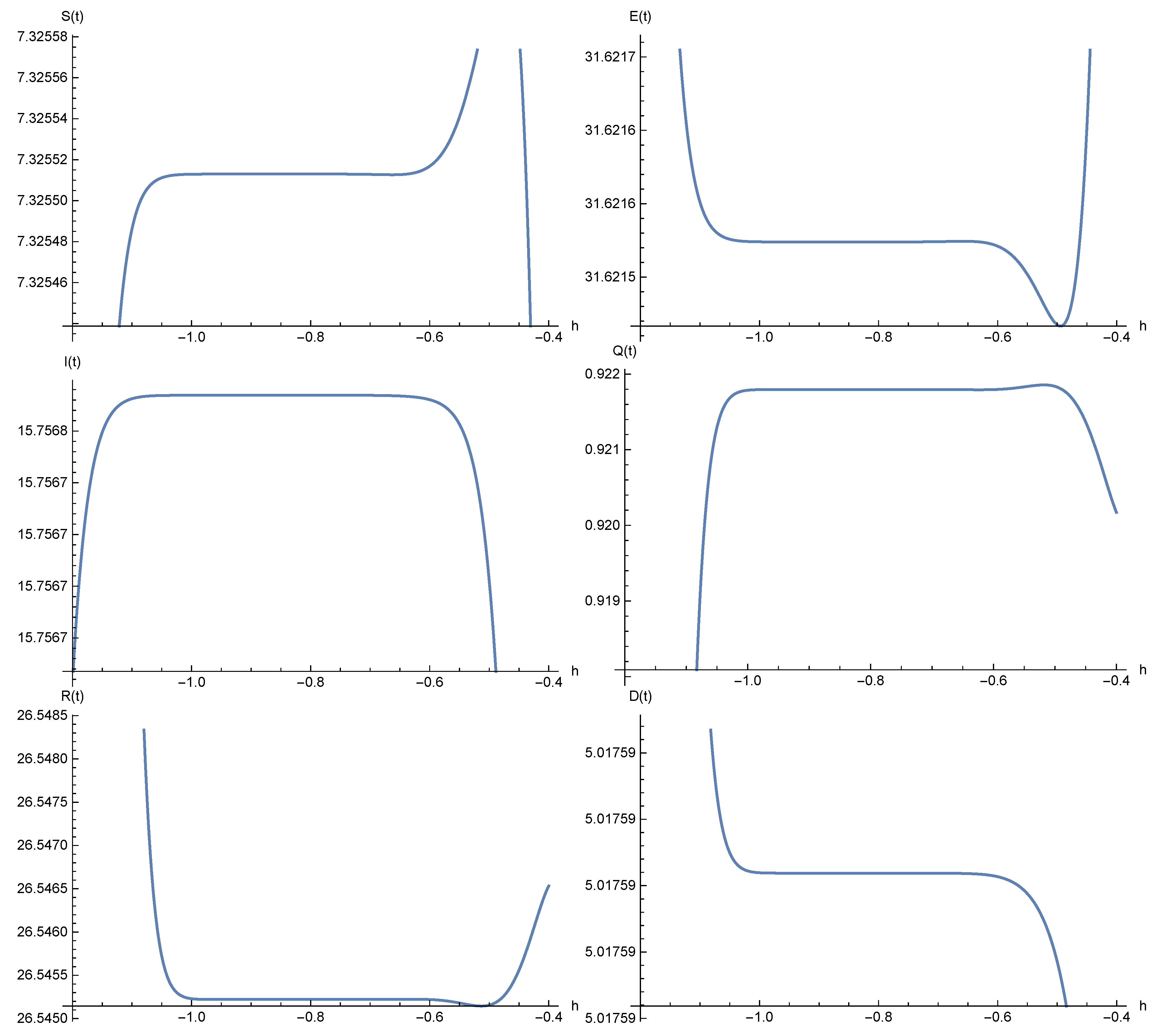
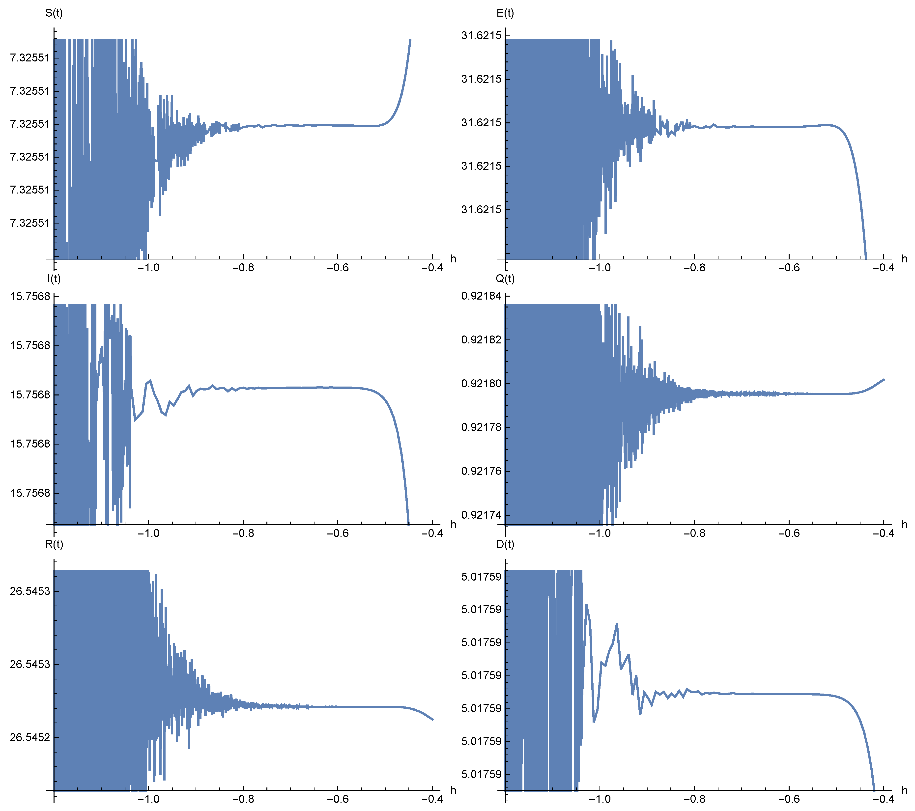
In this section, the numerical results of the HATM for solving the nonlinear fractional order model (4) are presented. As known in the HATM, we have some auxiliary functions and parameters that can help us find more accurate solutions with high-speed of convergence. In this method, the obtained solutions are based on t and such that the parameter can help identify and control the convergence region. To this aim, by plotting some -curves we can find these regions. In Figure 2, the -curves are presented for t = 0.2 and m = 15 . The convergence region for functions S , E , I , Q , R and D is 1 0.6 , , which is the parallel part of the -curve with the axis x. Additionally, by increasing the number of iterations of the HATM, we can plot more accurate -curves. In Figure 3, the -curves are plotted for m = 25 and we obtain:
0.7 S 0.5 , 0.55 Q 0.45 , 0.7 E 0.5 , 0.65 R 0.45 , 0.7 I 0.5 , 0.7 D 0.5 .
In Table 2, the numerical results obtained based on the DSA and using the CESTAC method are shown for t = 0.2 , ρ = 1 and = 0.8 . However, it is important to describe why we need to apply the DSA instead of the FPA. In the methods based on the FPA, generally we apply the traditional absolute error or residual error to show the accuracy of the method, but in these cases we need to know the exact solution and also in order to stop the numerical algorithm we need to apply a suitable termination criterion. Thus, instead of applying the methods based on the FPA, we propose methods based on the DSA. In this case, we apply the CESTAC method and the CADNA library to validate the numerical results. In the CESTAC method we use the difference between two successive approximations instead of the traditional absolute error. Additionally, we do not need to have positive small value such as ε and an important note is that we do not need to have the exact solution. Using this method, we can find the optimal number of iteration and the optimal approximation of the HATM for solving the mentioned model. According to Table 4, the optimal iteration is m o p t = 7 and the optimal approximations are:
S o p t = 0.732556 E + 001 , Q o p t = 0.91948 E + 000 , E o p t = 0.3162149 E + 002 , R o p t = 0.2654801 E + 002 , I o p t = 0.1575674 E + 002 , D o p t = 0.501759 E + 001 .
Sign @ . 0 in step 7 shows that the number of common significant digits between two successive approximations is zero. Thus, we can apply the difference between two successive approximations instead of traditional absolute error. Additionally, 24 numerical instabilities are reported by the CADNA library. In Table 3, the numerical results of the FPA based on Condition (1) for t = 0.2 and ε = 10 4 are presented. It is obvious that the stopping condition depends on the value of ε . In Table 4, the numbers of iterations for different values of ε are obtained. As we described before, the algorithm is stopped at the first steps for large values of ε . Additionally, for small values of ε we have large number of iterations. In Table 5, the numerical results are presented for t = 0.2 , ρ = 0.9 and = 0.6 based on the CESTAC method. Using this table we can find the optimal iteration m o p t = 10 and the following optimal approximations:
S o p t = 0.761582 E + 001 , Q o p t = 0.1916541 E + 002 , E o p t = 0.3076886 E + 002 , R o p t = 0.4576194 E + 002 , I o p t = 0.144270 E + 002 , D o p t = 0.528554 E + 001 .
In Figure 4, the approximate solution of the model using the HATM is demonstrated. We can see that by decreasing the number of susceptible people (red line), the quarantined people (dotted line) decreases, the infected people (dashed line) slowly decreases, the rate of exposed people (orange line) increases and after that slowly decreases, the death rate (green line) slowly increases, and the number of recovered people increases and then slowly increases. Thus, we have acceptable and logical results for the model.

9. Conclusions

Given the importance of modeling and controlling the COVID-19 pandemic, we focused on a nonlinear fractional order model of COVID-19. We applied the Caputo–Fabrizio fractional derivative to present a novel fractional order model. Some theorems were proven to show the existence of a solution and stability analysis. The HATM was used to solve the model numerically and the CESTAC method and the CADNA library were applied to validate the results. In order to show the accuracy of the results, instead of applying the absolute error we used the difference between two successive approximations. The main theorem of the CESTAC method enabled us to use the new termination criterion. This method is based on the DSA and using this method we can find the optimal iteration and the optimal approximation of the HATM for solving the fractional order model. A comparative study between the FPA and the DSA was presented to show the abilities of the CESTAC method and the CADNA library.

Author Contributions

Conceptualization, S.N., S.M. and J.J.N.; methodology, S.N.; software, S.N.; validation, S.N., S.M. and J.J.N.; formal analysis, S.N., S.M. and J.J.N.; investigation, S.N., S.M. and J.J.N.; resources, S.N.; data curation, S.N.; writing—original draft preparation, S.N.; writing—review and editing, S.N., S.M. and J.J.N.; visualization, S.N., S.M. and J.J.N.; supervision, S.N.; project administration, S.N.; funding acquisition, S.N. All authors have read and agreed to the published version of the manuscript.

Funding

The work of J.J.N. has been partially supported by the Xunta de Galicia under grant ED431C 2019/02, as well as by Instituto de Salud Carlos III and the Ministerio de Ciencia e Innovación of Spain, research grant COV20/00617. The work of S. Noeiaghdam has been supported by a grant from the Academic Council in the direction of the scientific school of Irkutsk National Research Technical University No. 14-NSH-RAN-2020.

Institutional Review Board Statement

Not applicable.

Informed Consent Statement

Not applicable.

Data Availability Statement

Not applicable.

Conflicts of Interest

The authors declare no conflict of interest.

References

  1. Coronavirus Disease (COVID-19) Pandemic. Available online: https://www.who.int/emergencies/diseases/novel-coronavirus-2019# (accessed on 2 March 2021).
  2. Srivastava, H.M.; Area, I.; Nieto, J.J. Power-series solutions of compartmental epidemiological models. Math. Biosci. Eng. 2021, 18. [Google Scholar] [CrossRef]
  3. Ndaïrou, F.; Area, I.; Nieto, J.J.; Silva, C.J.; Torres, D.F.M. Fractional model of COVID-19 applied to Galicia, Spain and Portugal. Chaos Solitons Fractals 2021, 144, 110652. [Google Scholar] [CrossRef]
  4. Bushnaq, S.; Saeed, T.; Torres, D.F.M.; Zeb, A. Control of COVID-19 dynamics through a fractional-order model. Alex. Eng. J. 2021, 60, 3587–3592. [Google Scholar] [CrossRef]
  5. Hu, F.; Huang, M.; Sun, J.; Zhang, X.; Liu, J. An analysis model of diagnosis and treatment for COVID-19 pandemic based on medical information fusion. Inf. Fusion 2021, 73, 11–21. [Google Scholar] [CrossRef]
  6. Gebremeskel, A.A.; Berhe, H.W.; Atsbaha, H.A. Mathematical modeling and analysis of COVID-19 epidemic and predicting its future situation in Ethiopia. Results Phys. 2021, 22, 103853. [Google Scholar] [CrossRef]
  7. Inc, M.; Acay, B.; Berhe, H.W.; Yusuf, A.; Khan, A.; Yao, S.-W. Analysis of novel fractional COVID-19 model with real-life data application. Results Phys. 2021, 23, 103968. [Google Scholar] [CrossRef]
  8. Zhang, W.; Zhang, C.; Bi, Y.; Yuan, L.; Jiang, Y.; Hasi, C.; Zhang, X.; Kong, X. Analysis of COVID-19 epidemic and clinical risk factors of patients under epidemiological Markov model. Results Phys. 2021, 22, 103881. [Google Scholar] [CrossRef]
  9. Galanis, G.; Hanieh, A. Incorporating Social Determinants of Health into Modelling of COVID-19 and other Infectious Diseases: A Baseline Socioeconomic Compartmental Model. Soc. Sci. Med. 2021, 274, 113794. [Google Scholar] [CrossRef]
  10. Panwar, V.S.; Sheik Uduman, P.S.; Gómez-Aguilar, J.F. Mathematical modeling of coronavirus disease COVID-19 dynamics using CF and ABC non-singular fractional derivatives. Chaos Solitons Fractals 2021, 145, 110757. [Google Scholar] [CrossRef]
  11. Naik, P.A.; Zu, J.; Owolabi, K.M. Modeling the mechanics of viral kinetics under immune control during primary infection of HIV-1 with treatment in fractional order. Phys. A Stat. Mech. Appl. 2020, 545, 123816. [Google Scholar] [CrossRef]
  12. Ghanbari, B.; Günerhan, H.; Srivastava, H.M. An application of the Atangana–Baleanu fractional derivative in mathematical biology: A three-species predator-prey model. Chaos Solitons Fractals 2020, 138, 109910. [Google Scholar] [CrossRef]
  13. Günerhan, H.; Dutta, H.; Dokuyucu, M.A.; Adel, W. Analysis of a fractional HIV model with Caputo and constant proportional Caputo operators. Chaos Solitons Fractals 2020, 139, 110053. [Google Scholar] [CrossRef]
  14. Noeiaghdam, S.; Sidorov, D. Caputo–Fabrizio Fractional Derivative to Solve the Fractional Model of Energy Supply-Demand System. Math. Model. Eng. Probl. 2020, 7, 359–367. [Google Scholar] [CrossRef]
  15. Naik, P.A.; Yavuz, M.; Zu, J. The role of prostitution on HIV transmission with memory: A modeling approach. Alex. Eng. J. 2020, 59, 2513–2531. [Google Scholar] [CrossRef]
  16. Naik, P.A.; Zu, J.; Owolabi, K.M. Global dynamics of a fractional order model for the transmission of HIV epidemic with optimal control. Chaos Solitons Fractals 2020, 138, 109826. [Google Scholar] [CrossRef]
  17. Suleman, M.; Lu, D.; He, J.H.; Farooq, U.; Noeiaghdam, S.; Chandio, F.A. Elzaki Projected Differential Transform method for Fractional order System of Linear and Nonlinear Fractional Partial Differential Equation. Fractals 2018, 26, 1850041. [Google Scholar]
  18. Noeiaghdam, S. A novel technique to solve the modified epidemiological model of computer viruses. SeMA J. 2019, 76, 97–108. [Google Scholar] [CrossRef]
  19. Hattaf, K.; Mohsen, A.A.; Harraq, J.; Achtaich, N. Modeling the dynamics of COVID-19 with carrier effect and environmental contamination. Int. J. Model. Simul. Sci. Comput. 2021. [Google Scholar] [CrossRef]
  20. Abboubakar, H.; Kumar, P.; Rangaig, N.A.; Kumar, S. A malaria model with Caputo–Fabrizio and Atangana–Baleanu derivatives. Int. J. Model. Simul. Sci. Comput. 2021, 2021 12, 2150013. [Google Scholar] [CrossRef]
  21. Liao, S.J. Beyond Perturbation: Introduction to Homotopy Analysis Method; Chapman & Hall/CRC Press: Boca Raton, FL, USA, 2003. [Google Scholar]
  22. Liao, S.J. Homotopy Analysis Method in Nonlinear Differential Equations; Higher Education Press: Beijing, China; Springer: Berlin/Heidelberg, Germany, 2012. [Google Scholar]
  23. Liao, S.J. The Proposed Homotopy Analysis Techniques for the Solution of Nonlinear Problems. Ph.D. Thesis, Shanghai Jiao Tong University, Shanghai, China, 1992. [Google Scholar]
  24. Noeiaghdam, S.; Fariborzi Araghi, M.A. A novel approach to find optimal parameter in the homotopy-regularization method for solving integral equations. Appl. Math. Inf. Sci. 2020, 14, 1–8. [Google Scholar]
  25. Noeiaghdam, S.; Fariborzi Araghi, M.A.; Abbasbandy, S. Finding optimal convergence control parameter in the homotopy analysis method to solve integral equations based on the stochastic arithmetic. Numer. Algorithms 2019, 81, 237. [Google Scholar] [CrossRef]
  26. Noeiaghdam, S.; Fariborzi Araghi, M.A. Homotopy regularization method to solve the singular Volterra integral equations of the first kind. Jordan J. Math. Stat. 2018, 11, 1–12. [Google Scholar]
  27. Fariborzi Araghi, M.A.; Noeiaghdam, S. A novel technique based on the homotopy analysis method to solve the first kind Cauchy integral equations arising in the theory of airfoils. J. Interpolat. Approx. Sci. Comput. 2016, 2016, 1–13. [Google Scholar] [CrossRef] [Green Version]
  28. Noeiaghdam, S.; Suleman, M.; Budak, H. Solving a modified non-linear epidemiological model of computer viruses by homotopy analysis method. Math. Sci. 2018, 12, 211–222. [Google Scholar] [CrossRef] [Green Version]
  29. Vignes, J. A stochastic arithmetic for reliable scientific computation. Math. Comput. Simul. 1993, 35, 233–261. [Google Scholar] [CrossRef]
  30. Laboratoire d’Informatique de Paris 6. Available online: https://www-pequan.lip6.fr/ (accessed on 10 December 2020).
  31. Chesneaux, J.M. CADNA, an ADA tool for round–off error analysis and for numerical debugging. In Proceedings of the Congress on ADA, Aerospace, Barcelona, Spain, 20–25 May 1990. [Google Scholar]
  32. Chesneaux, J.M.; Jézéquel, F. Dynamical control of computations using the Trapezoidal and Simpson’s rules. J. Univers. Comput. Sci. 1998, 4, 2–10. [Google Scholar]
  33. Graillat, S.; Jézéquel, F.; Wang, S.; Zhu, Y. Stochastic arithmetic in multi precision. Math. Comput. Sci. 2011, 5, 359–375. [Google Scholar] [CrossRef]
  34. Graillat, S.; Jézéquel, F.; Picot, R. Numerical Validation of Compensated Summation Algorithms with Stochastic Arithmetic. Electron. Notes Theor. Comput. Sci. 2015, 317, 55–69. [Google Scholar] [CrossRef]
  35. Jézéquel, F.; Mecanique, C.R. A dynamical strategy for approximation methods. Comptes Rendus Mec. 2006, 334, 362–367. [Google Scholar] [CrossRef] [Green Version]
  36. Noeiaghdam, S.; Sidorov, D.; Wazwaz, A.M.; Sidorov, N.; Sizikov, V. The numerical validation of the Adomian decomposition method for solving Volterra integral equation with discontinuous kernel using the CESTAC method. Mathematics 2021, 9, 260. [Google Scholar] [CrossRef]
  37. Noeiaghdam, S.; Sidorov, D.; Zamyshlyaeva, A.; Tynda, A.; Dreglea, A. A valid dynamical control on the reverse osmosis system using the CESTAC method. Mathematics 2021, 9, 48. [Google Scholar] [CrossRef]
  38. Noeiaghdam, S.; Fariborzi Araghi, M.A. A novel algorithm to evaluate definite integrals by the Gauss-Legendre integration rule based on the stochastic arithmetic: Application in the model of osmosis system. Math. Model. Eng. Probl. 2020, 7, 577–586. [Google Scholar] [CrossRef]
  39. Noeiaghdam, S.; Dreglea, A.; He, J.H.; Avazzadeh, Z.; Suleman, M.; Fariborzi Araghi, M.A.; Sidorov, D.; Sidorov, N. Error estimation of the homotopy perturbation method to solve second kind Volterra integral equations with piecewise smooth kernels: Application of the CADNA library. Symmetry 2020, 12, 1730. [Google Scholar] [CrossRef]
  40. Noeiaghdam, S.; Sidorov, D.; Sizikov, V.; Sidorov, N. Control of accuracy on Taylor-collocation method to solve the weakly regular Volterra integral equations of the first kind by using the CESTAC method. Appl. Comput. Math. Int. J. 2020, 19, 81. [Google Scholar]
  41. Noeiaghdam, S.; Fariborzi Araghi, M.A. Valid implementation of the Sinc-collocation method to solve the linear integral equations by CADNA library. J. Math. Model. 2019, 7, 63–84. [Google Scholar]
  42. Noeiaghdam, S.; Sidorov, D.; Muftahov, D.I.; Zhukov, A.V. Control of Accuracy on Taylor-Collocation Method for Load Leveling Problem. Bull. Irkutsk State Univ. Ser. Math. 2019, 30, 59–72. [Google Scholar] [CrossRef]
  43. Caputo, M.; Fabrizio, M. A new definition of fractional derivative without singular kernel. Prog. Fract. Differ. Appl. 2015, 1, 73–85. [Google Scholar]
  44. Losada, J.; Nieto, J.J. Properties of the new fractional derivative without singular kernel. Prog. Fract. Differ. Appl. 2015, 1, 87–92. [Google Scholar]
  45. Abdeljawad, T.; Baleanu, D. On fractional derivatives with exponential kernel and their discrete versions. Rep. Math. Phys. 2017, 80, 11–27. [Google Scholar] [CrossRef] [Green Version]
  46. Belgacem, F.B.M.; Karaballi, A.A.; Kalla, S.L. Analytical investigations of the Sumudu transform and applications to integral production equations. Math. Probl. Eng. 2003, 3, 103–118. [Google Scholar] [CrossRef] [Green Version]
  47. Bodkhe, D.S.; Panchal, S.K. On Sumudu transform of fractional derivatives and its applications to fractional differential equations. Asian J. Math. Comput. Res. 2016, 11, 69–77. [Google Scholar]
  48. Shah, K.; Junaid, N.A.M. Extraction of Laplace, Sumudu, Fourier and Mellin transform from the natural transform. J. Appl. Environ. Biol. Sci. 2015, 5, 1–10. [Google Scholar]
  49. Watugala, G.K. Sumudu transform: A new integral transform to solve differential equations and control engineering problems. Int. J. Math. Educ. Sci. Technol. 1993, 24, 35–43. [Google Scholar] [CrossRef]
  50. Wang, J.; Zhou, Y.; Medved, M. Picard and weakly Picard operators technique for nonlinear differential equations in Banach spaces. J. Math. Anal. Appl. 2012, 389, 261–274. [Google Scholar] [CrossRef] [Green Version]
  51. Chatterjee, K.; Chatterjee, K.; Kumar, A.; Shankar, S. Healthcare impact of COVID-19 epidemic in India: A stochastic mathematical model. Med. J. Armed Forces India 2020, 76, 147–155. [Google Scholar] [CrossRef]
  52. Sarkar, K.; Khajanchi, S.; Nieto, J.J. Modeling and forecasting the COVID-19 pandemic in India. Chaos Solitons Fractals 2020, 139, 110049. [Google Scholar] [CrossRef]
  53. Vignes, J. Discrete Stochastic Arithmetic for Validating Results of Numerical Software. Spec. Issue Numer. Algorithms 2004, 7, 377–390. [Google Scholar] [CrossRef]
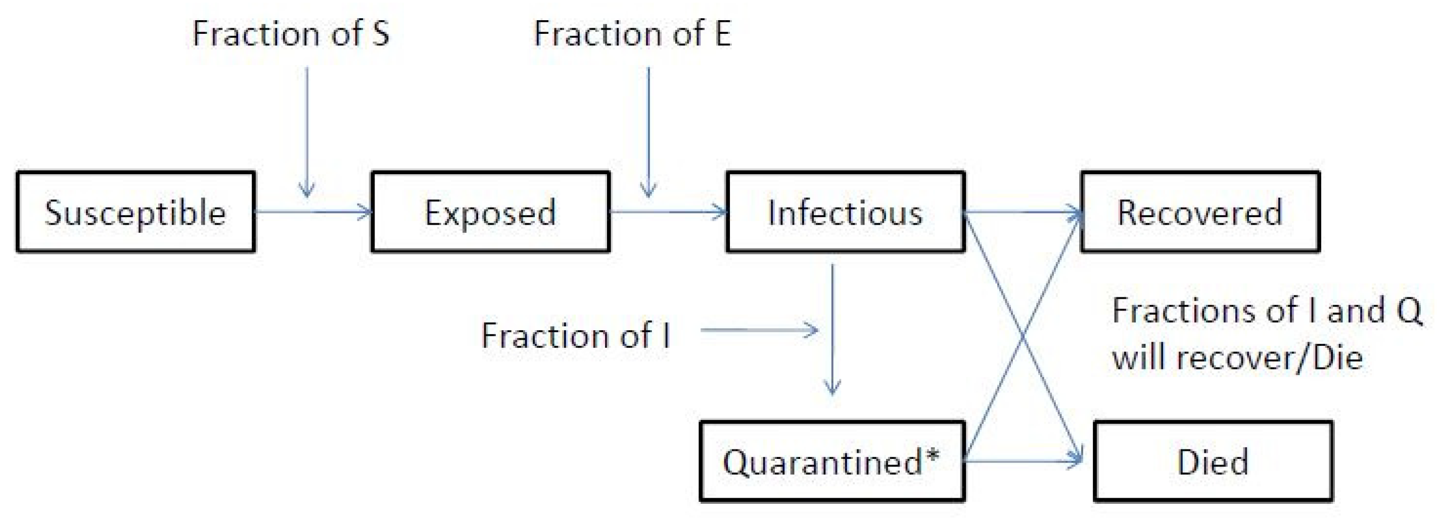
Figure 1. The model of COVID-19 [51].
Mathematics 09 01321 g001
Figure 2. The -curves of the approximate solutions obtained form HATM for t = 0.2 and m = 15 .
Mathematics 09 01321 g002
Figure 3. The -curves of the approximate solutions obtained form HATM for t = 0.2 and m = 25 .
Mathematics 09 01321 g003
Figure 4. The approximate solution for m = 15 , = 0.8 .
Mathematics 09 01321 g004
Table 1. List of parameters and functions [51].
ParametersValues
Incubation Period 1 ε Mean= 5.1 days
Infectious Period 1 γ Mean= 7 days
Basic Reproduction Number R 0 Mean= 2.28
Mean Death Rate 0.43 %
Active Cases Quarantined q0.01
Period Quarantined q t 14 days
Quarantined Cases S 0 20
Recovered Cases R 0 12
Deaths D 0 5
Exposed Cases E 0 20
Infected Cases I 0 15
Quarantined Cases Q 0 15
Table 2. Numerical results based on the DSA and using the CESTAC method for t = 0.2 , ρ = 1 and = 0.8 .
mApproximate SolutionsDifference between Two Iterations
1 4.365721 4.365721
35.00683 35.00683
15.39427 15.39427
18.58639 18.58639
45.94279 45.94279
5.020640 5.020640
2 7.081621 2.71589
31.93003 3.07679
15.70567 0.31139
12.3250 30.9114
15.1206 30.82215
5.013390 0.7249 × 10 2
3 7.329236 0.24761
31.62606 0.30397
15.75156 0.45893 × 10 1
2.0715 14.3966
29.53187 14.4112
5.01834 0.495 × 10 2
4 7.33754 0.831 × 10 2
31.61051 0.155 × 10 1
15.75638 0.482 × 10 2
1.0558 3.1274
26.40971 3.1221
5.017514 0.834 × 10 3
5 7.32929 0.825 × 10 2
31.61790 0.738 × 10 2
15.75678 0.39 × 10 3
1.00038 0.5541 × 10 1
26.46585 0.561 × 10 1
5.01755 0.4 × 10 4
6 7.32617 0.311 × 10 2
31.62090 0.2998352 × 10 2
15.75674 0.3 × 10 4
0.91942 0.8095 × 10 1
26.5475 0.8165 × 10 1
5.01759 0.3 × 10 4
7 7.32556 0.6 × 10 3
31.62149 0.59 × 10 3
15.75674 @ . 0
91948 0.6 × 10 4
26.54801 0.50 × 10 3
5.01759 @ . 0
Table 3. Numerical results based on the FPA and Condition (1) for t = 0.2 , ρ = 1 , = 0.8 and ε = 10 4 .
mApproximate SolutionsDifference between Two Iterations
1 4.365721 4.365721
35.00683 35.00683
15.39427 15.39427
18.58639 18.58639
45.94279 45.94279
5.020640 5.020640
2 7.081621 2.71589
31.93003 3.07679
15.70567 0.31139
12.3250 30.9114
15.1206 30.82215
5.013390 0.7249 × 10 2
3 7.329236 0.24761
31.62606 30397
15.75156 45893 × 10 1
2.0715 14.3966
29.53187 14.4112
5.01834 0.495 × 10 2
4 7.33754 0.831 × 10 2
31.61051 0.155 × 10 1
15.75638 0.482 × 10 2
1.0558 3.1274
26.40971 3.1221
5.017514 0.834 × 10 3
5 0.732929 0.825 × 10 2
31.61790 0.738 × 10 2
15.75678 0.39 × 10 3
1.00038 0.5541 × 10 1
26.46585 0.561 × 10 1
5.01755 0.4 × 10 4
Table 4. Number of iterations based on the FPA and Condition (1) for various ε and t = 0.2 , ρ = 1 , = 0.8 .
ε Small Values 10 5 10 4 10 1 0.5Large Values
m > > 9 95311
Table 5. Numerical results based on the DSA and using the CESTAC method for t = 0.2 , ρ = 0.9 and = 0.6 .
mApproximate SolutionsDifference between Two Iterations
10.64160380.6416040
35.7572135.75721
14.3051914.30519
21.3383921.33840
47.6399947.63999
5.2941205.294120
28.2905081.87447
30.375355.38186
14.486190.18099
34.0154312.67704
5.9242941.757
5.184150.10996
37.427540.86296
31.07350.69816
14.44400 0.4218 × 10 1
34.8834 0.86797 × 10 2
60.98040 0.17375 × 10 1
5.3737540.18960
    ⋮    ⋮     ⋮
97.61575 0.32 × 10 3
30.7691 0.1 × 10 3
14.42713 0.19 × 10 3
19.1588 0.43 × 10 3
45.76194 0.2 × 10 4
5.33333 0.6258 × 10 1
107.61582 0.7 × 10 4
30.76886@.0
14.4270 0.7 × 10 4
19.16541 0.6 × 10 4
45.76194@.0
5.28554 0.4779 × 10 1
Publisher’s Note: MDPI stays neutral with regard to jurisdictional claims in published maps and institutional affiliations.