Author Contributions
Conceptualization, L.R.-M., S.B., M.D.; methodology, L.R.-M., S.B., M.D.; software, L.R.-M., S.B., M.D.; validation, L.R.-M., S.B., M.D.; investigation, L.R.-M., S.B., M.D.; data curation, L.R.-M., S.B., M.D.; writing—original draft preparation, L.R.-M., S.B., M.D.; writing—review and editing, L.R.-M., S.B., M.D.; visualization, L.R.-M., S.B., M.D.; funding acquisition, S.B., M.D. All authors have read and agreed to the published version of the manuscript.
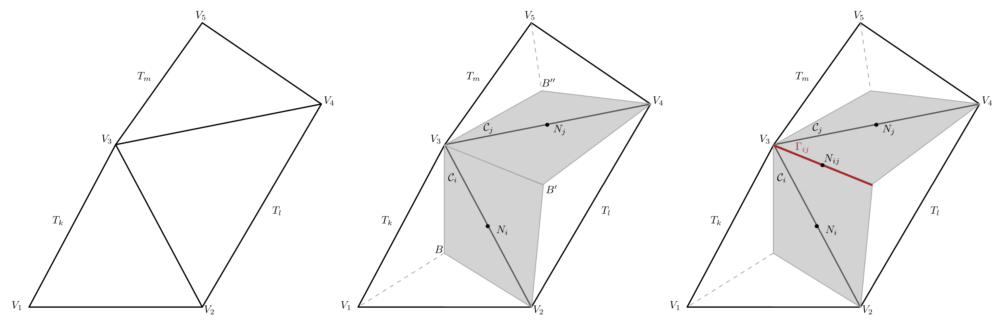
Figure 1.
Construction of face-type dual elements from a 2D triangular mesh. (Left) primal elements , , with vertex . (Center) dual interior cells , (shadowed in grey); white triangles correspond to boundary cells. (Right) boundary face, (highlighted in red), between the dual elements and .
Figure 1.
Construction of face-type dual elements from a 2D triangular mesh. (Left) primal elements , , with vertex . (Center) dual interior cells , (shadowed in grey); white triangles correspond to boundary cells. (Right) boundary face, (highlighted in red), between the dual elements and .
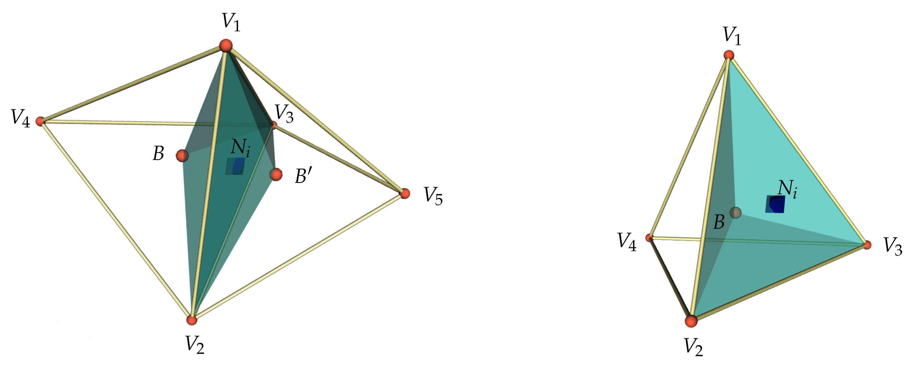
Figure 2.
Staggered dual mesh in 3D. (Left) interior finite volume. (Right) boundary finite volume.
Figure 2.
Staggered dual mesh in 3D. (Left) interior finite volume. (Right) boundary finite volume.
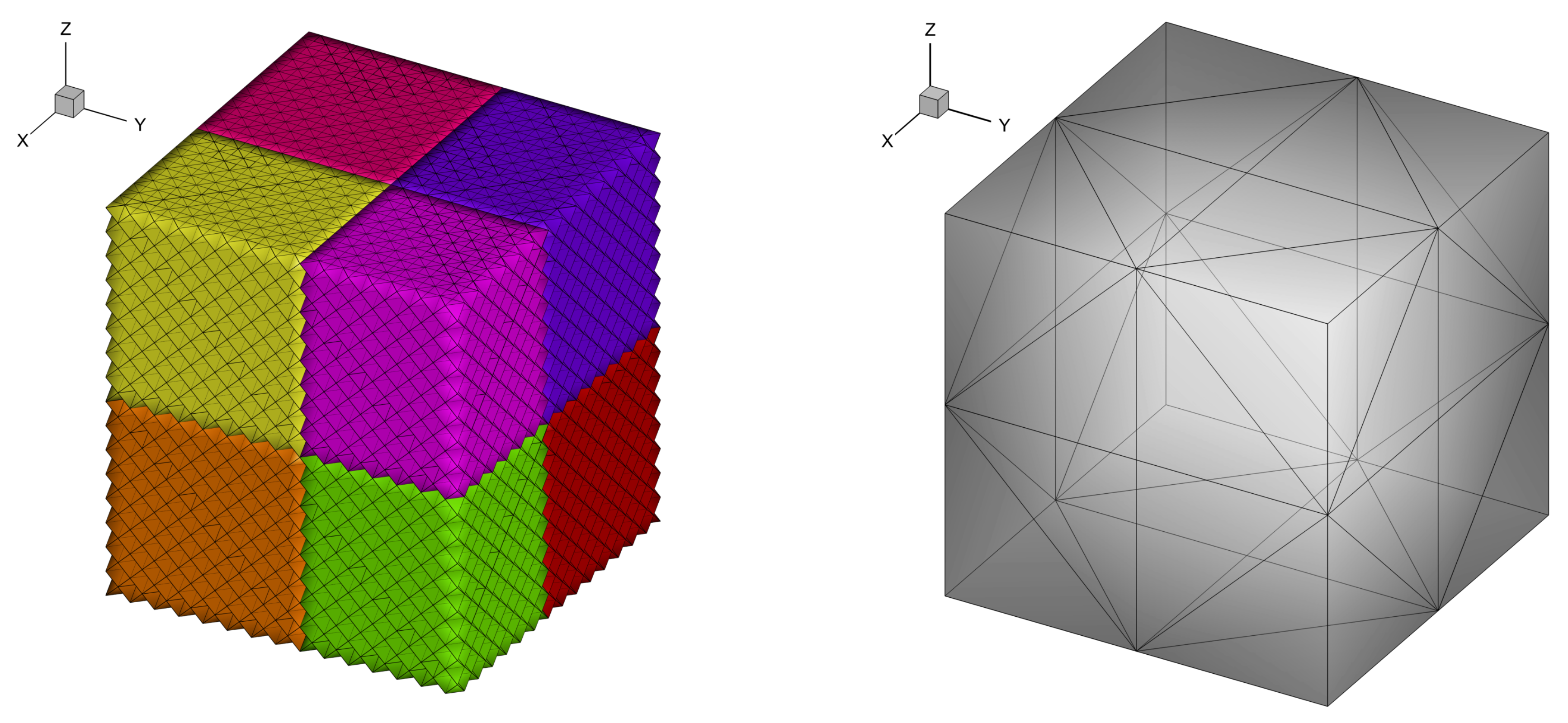
Figure 3.
(Left) Split-Cartesian mesh of hexahedra and MPI ranks. (Right) Detail of the division of hexahedra into tetrahedra.
Figure 3.
(Left) Split-Cartesian mesh of hexahedra and MPI ranks. (Right) Detail of the division of hexahedra into tetrahedra.
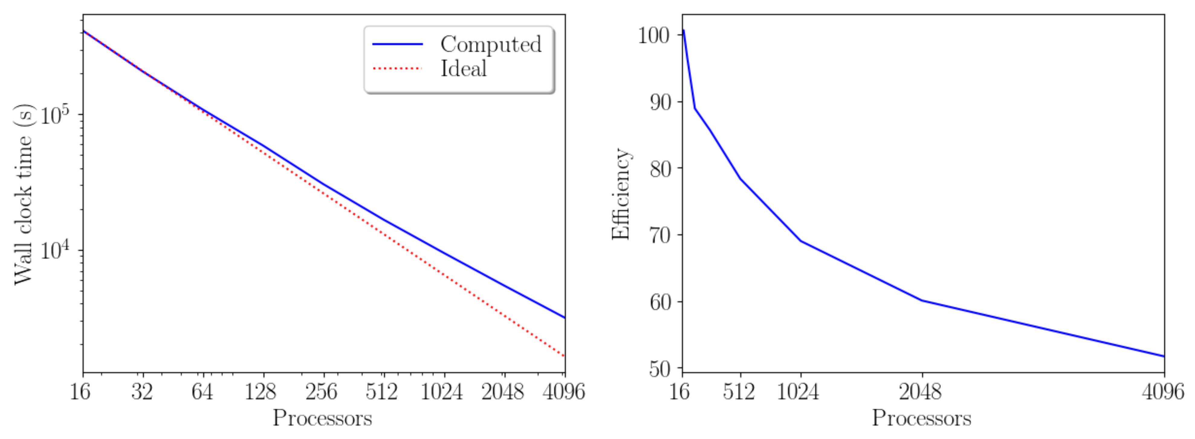
Figure 4.
(Left) Wall-clock time as a function of the processor number to solve the TGV benchmark with 83,886,080 primal elements. (Right) Efficiency.
Figure 4.
(Left) Wall-clock time as a function of the processor number to solve the TGV benchmark with 83,886,080 primal elements. (Right) Efficiency.
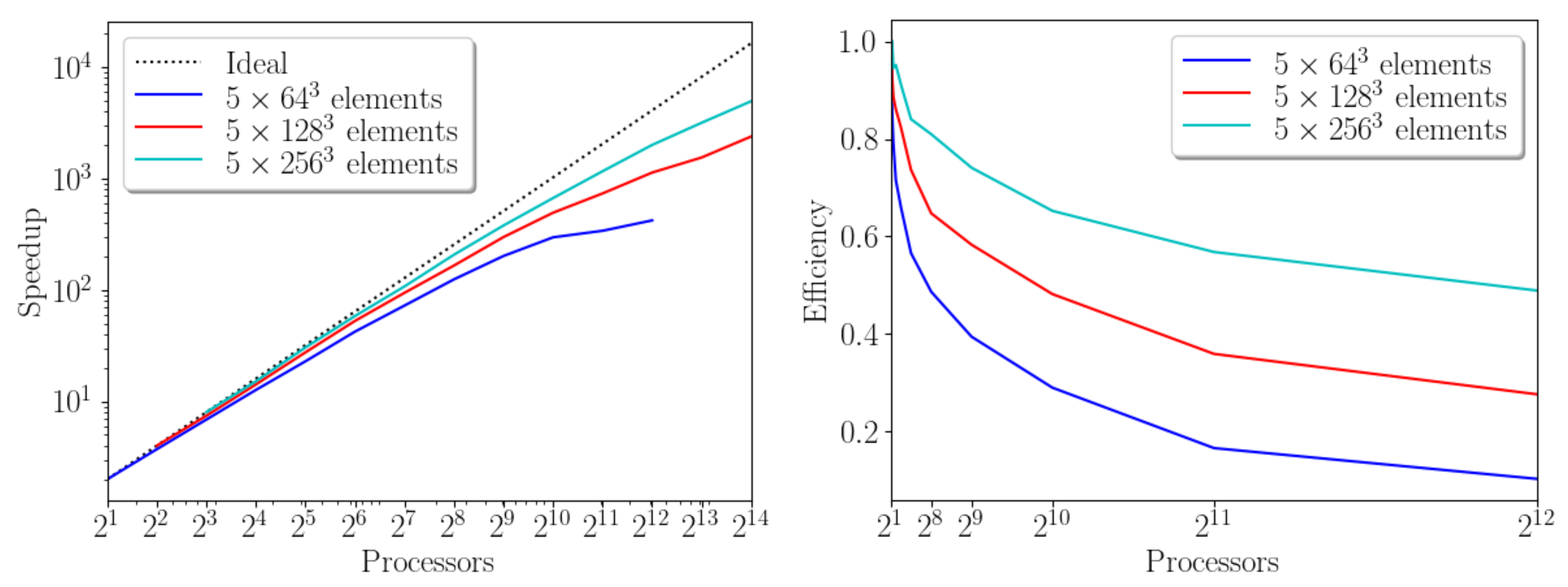
Figure 5.
Speedup graph (left) comparing the measured and the ideal wall-clock time from 16 to 4096 CPUs, and efficiency graph (right) considering three different meshes: tetrahedra (in blue), tetrahedra (in green), and tetrahedra (in cyan).
Figure 5.
Speedup graph (left) comparing the measured and the ideal wall-clock time from 16 to 4096 CPUs, and efficiency graph (right) considering three different meshes: tetrahedra (in blue), tetrahedra (in green), and tetrahedra (in cyan).
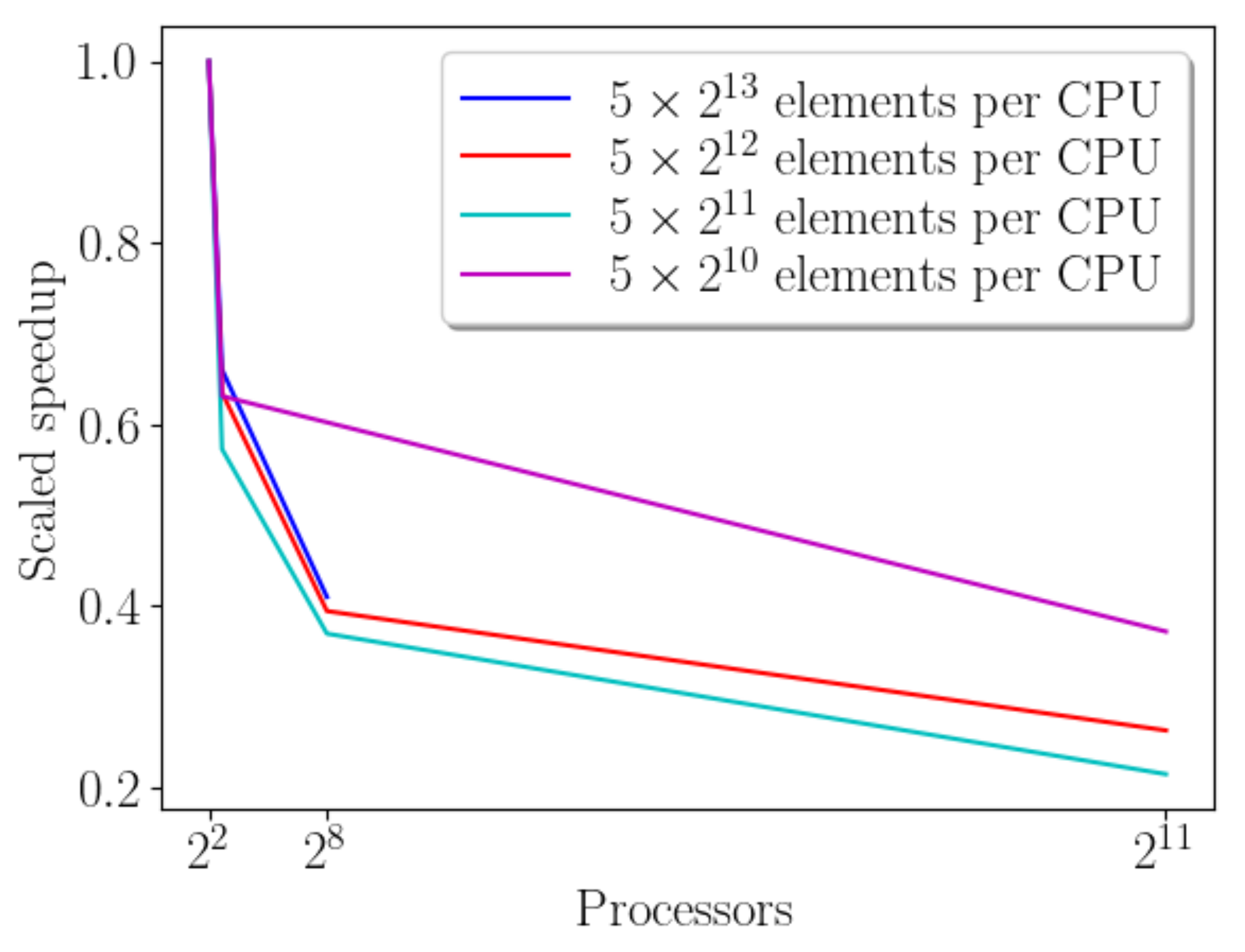
Figure 6.
Scaled speedup of a parallel simulation of the TGV benchmark. The number of elements per processor remains constant.
Figure 6.
Scaled speedup of a parallel simulation of the TGV benchmark. The number of elements per processor remains constant.
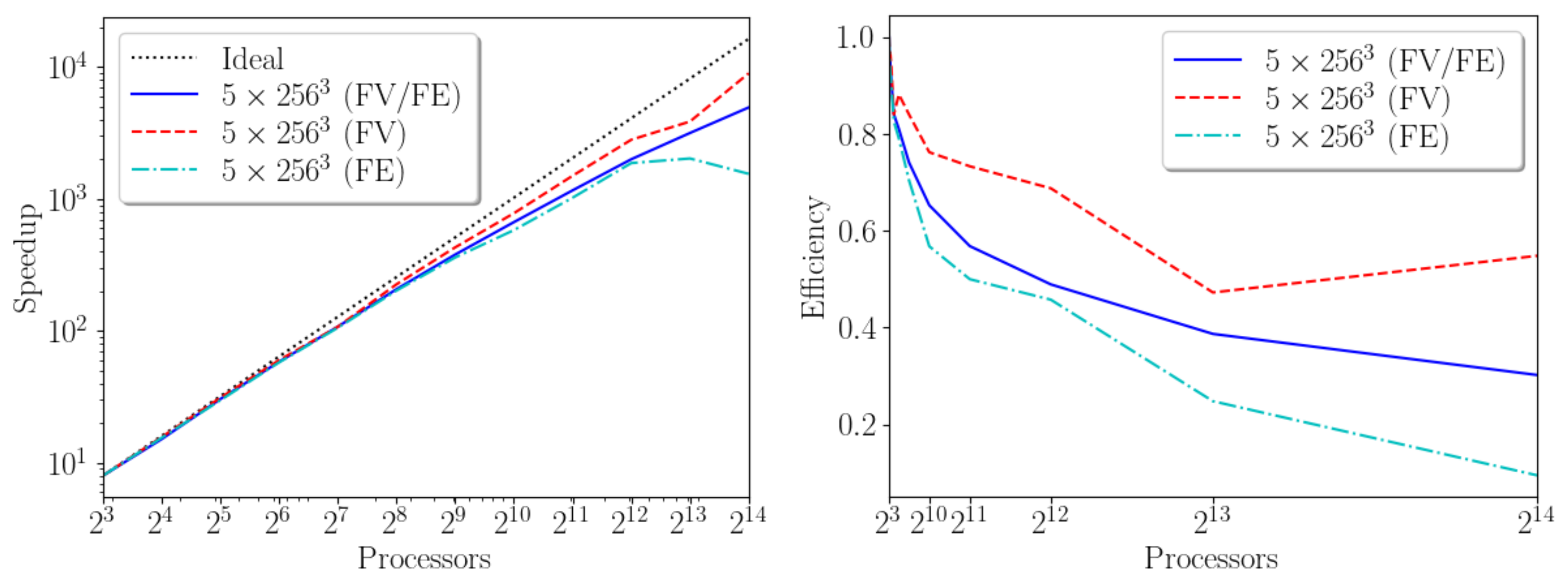
Figure 7.
Comparative of the wall-clock time (left) and the efficiency (right) considering the hybrid FV/FE method (solid blue line), finite volumes (dashed red line) and finite elements (dash-dotted cyan line) to solve the TGV benchmark with 83,886,080 primal elements.
Figure 7.
Comparative of the wall-clock time (left) and the efficiency (right) considering the hybrid FV/FE method (solid blue line), finite volumes (dashed red line) and finite elements (dash-dotted cyan line) to solve the TGV benchmark with 83,886,080 primal elements.
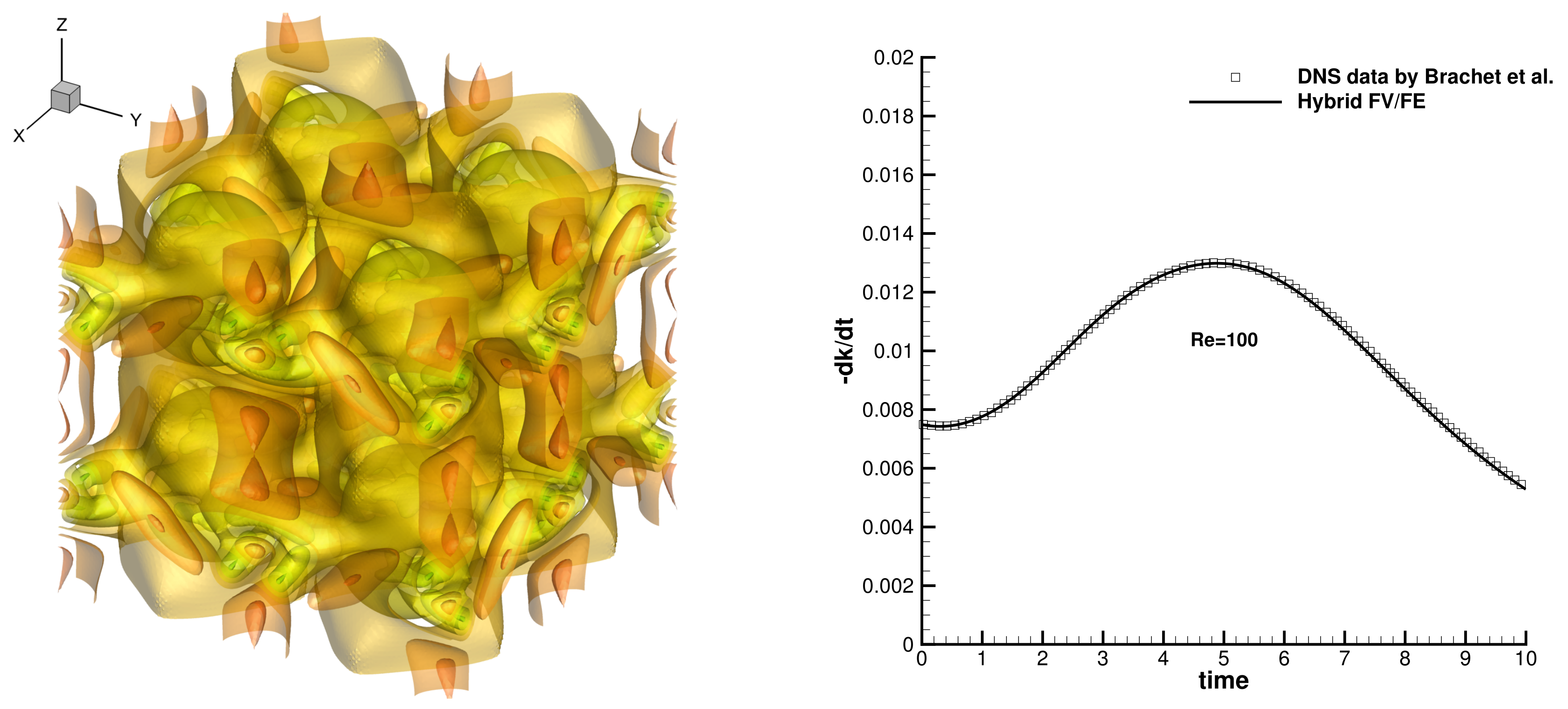
Figure 8.
Three-dimensional Taylor-Green vortex with
. Pressure isosurfaces at time
for
,
(
left) and 1D plot of the total kinetic energy dissipation rate compared against the DNS data in [
93] (
right).
Figure 8.
Three-dimensional Taylor-Green vortex with
. Pressure isosurfaces at time
for
,
(
left) and 1D plot of the total kinetic energy dissipation rate compared against the DNS data in [
93] (
right).
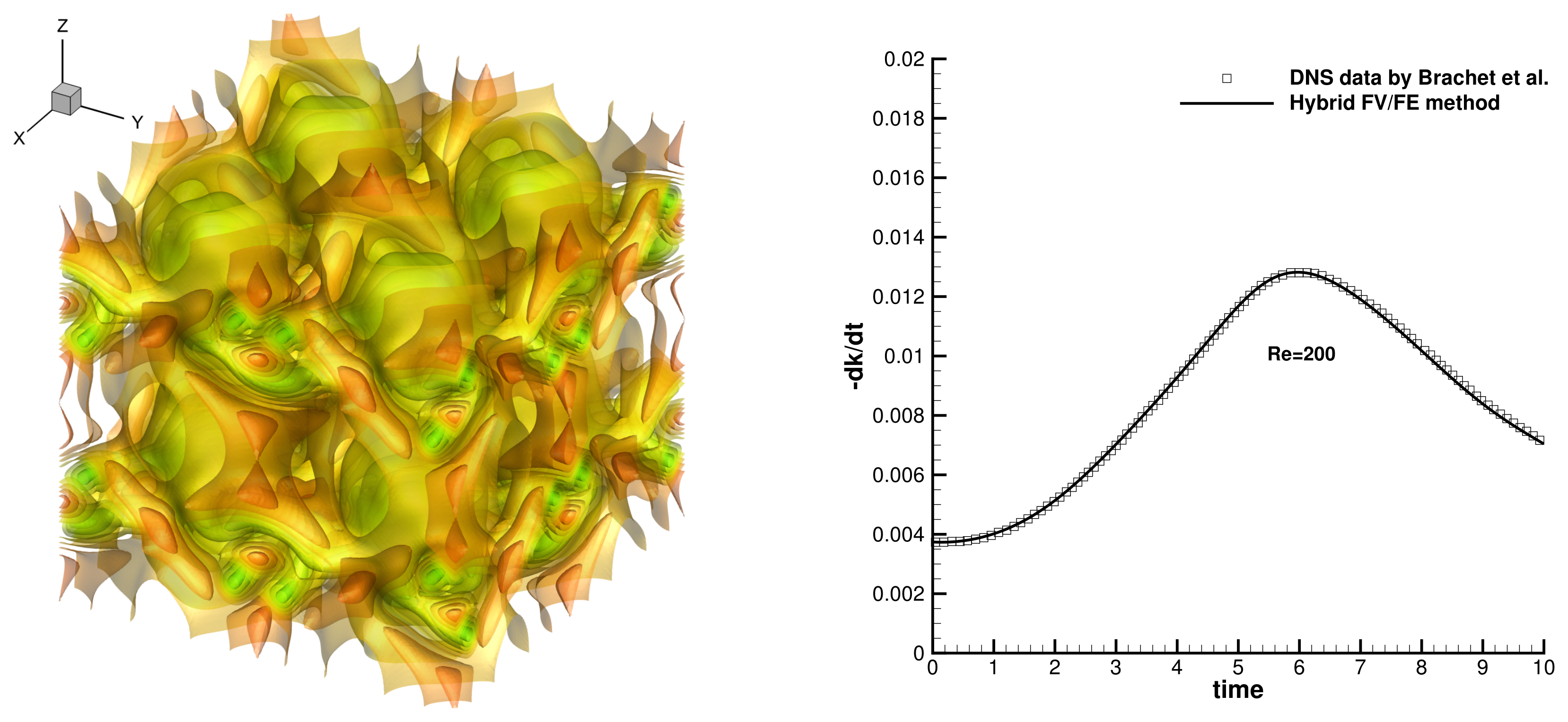
Figure 9.
Three-dimensional Taylor-Green vortex with
. Pressure isosurfaces at time
for
,
(
left) and 1D plot of the total kinetic energy dissipation rate compared against the DNS data in [
93] (
right).
Figure 9.
Three-dimensional Taylor-Green vortex with
. Pressure isosurfaces at time
for
,
(
left) and 1D plot of the total kinetic energy dissipation rate compared against the DNS data in [
93] (
right).
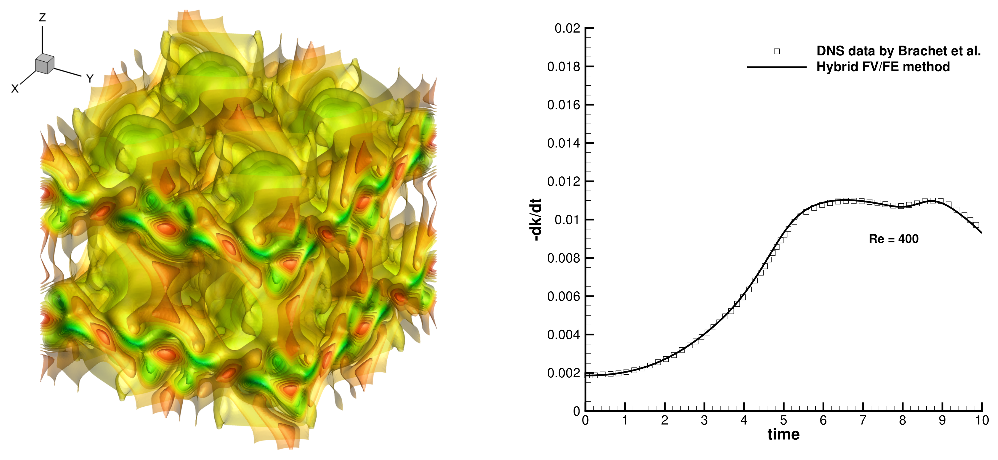
Figure 10.
Three-dimensional Taylor-Green vortex with
. Pressure isosurfaces at time
for
,
(
left) and 1D plot of the total kinetic energy dissipation rate compared against the DNS data in [
93] (
right).
Figure 10.
Three-dimensional Taylor-Green vortex with
. Pressure isosurfaces at time
for
,
(
left) and 1D plot of the total kinetic energy dissipation rate compared against the DNS data in [
93] (
right).
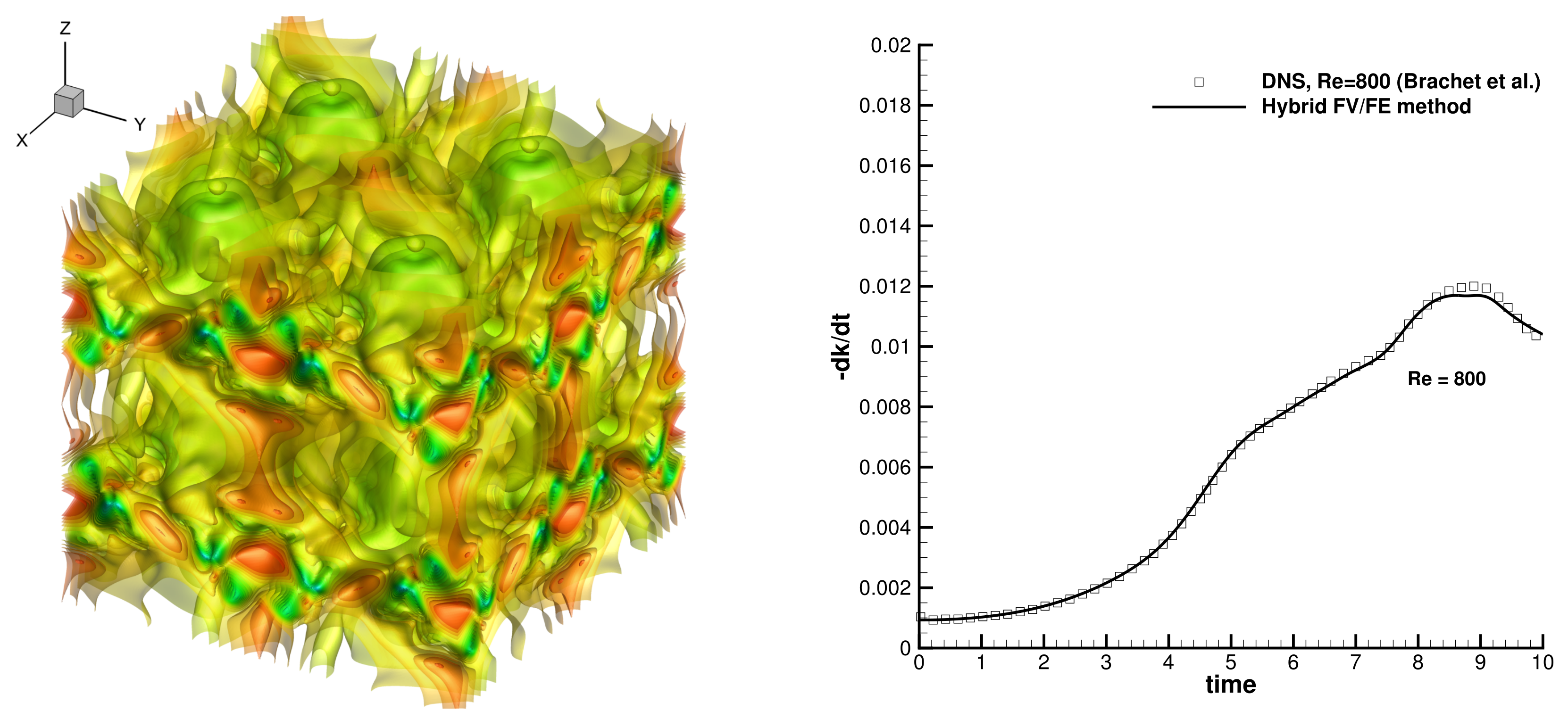
Figure 11.
Three-dimensional Taylor-Green vortex with
. Pressure isosurfaces at time
for
,
(
left) and 1D plot of the total kinetic energy dissipation rate compared against the DNS data in [
93] (
right).
Figure 11.
Three-dimensional Taylor-Green vortex with
. Pressure isosurfaces at time
for
,
(
left) and 1D plot of the total kinetic energy dissipation rate compared against the DNS data in [
93] (
right).
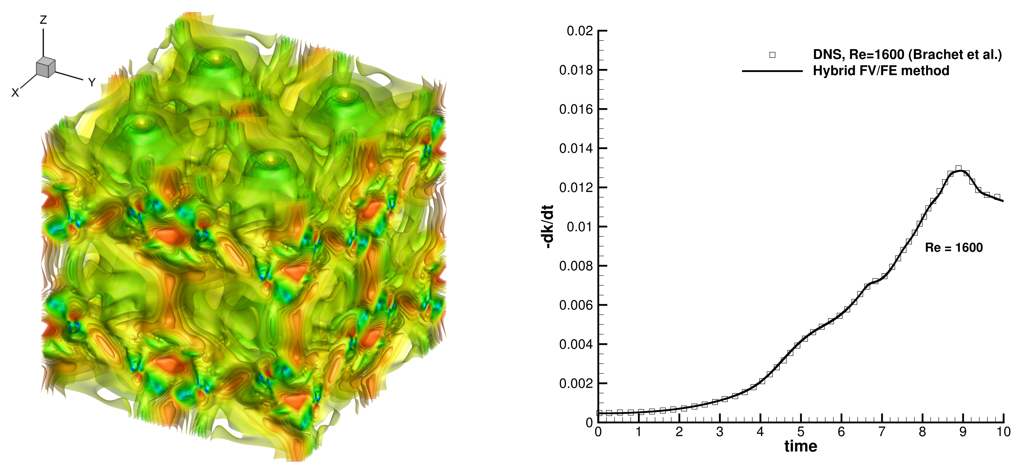
Figure 12.
Three-dimensional Taylor-Green vortex with
. Pressure isosurfaces at time
(
left) and 1D plot of the total kinetic energy dissipation rate compared against the DNS data in [
93] (
right).
Figure 12.
Three-dimensional Taylor-Green vortex with
. Pressure isosurfaces at time
(
left) and 1D plot of the total kinetic energy dissipation rate compared against the DNS data in [
93] (
right).
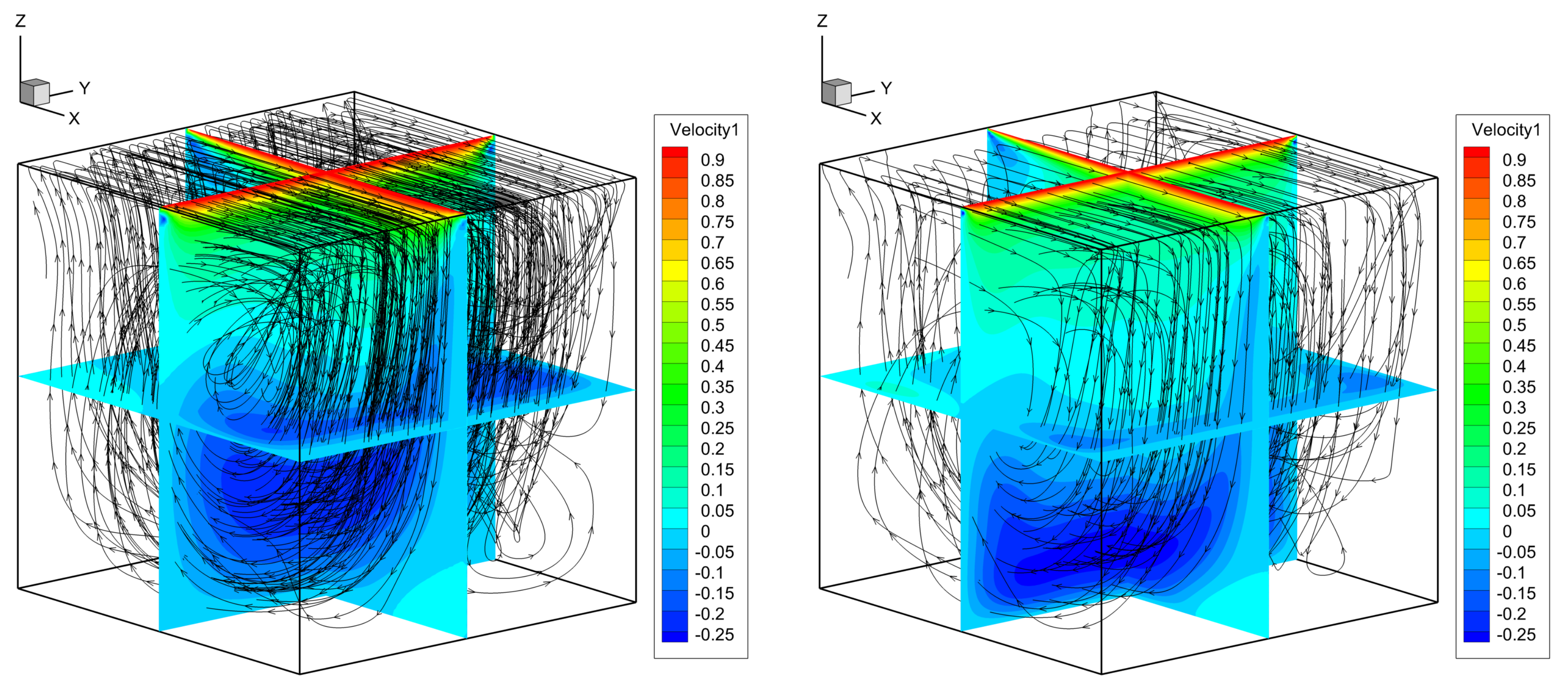
Figure 13.
Streamlines and velocity contour colors (m/s) for the three–dimensional lid–driven cavity at (left) and (right) at time .
Figure 13.
Streamlines and velocity contour colors (m/s) for the three–dimensional lid–driven cavity at (left) and (right) at time .
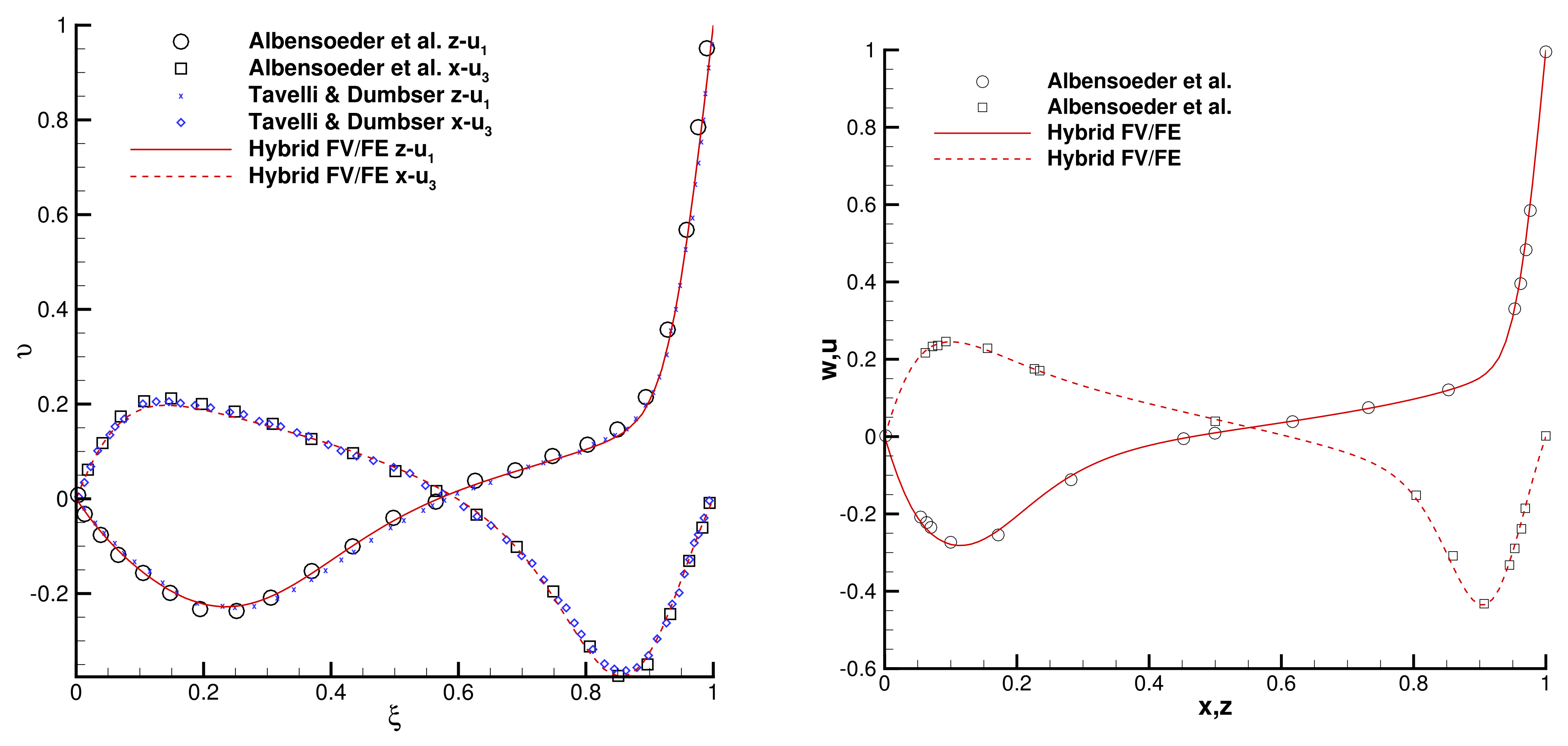
Figure 14.
1D cuts through the numerical solution for the 3D lid–driven cavity at time
and comparison with available numerical reference solutions in [
48,
94]. (
Left)
. (
Right)
.
Figure 14.
1D cuts through the numerical solution for the 3D lid–driven cavity at time
and comparison with available numerical reference solutions in [
48,
94]. (
Left)
. (
Right)
.
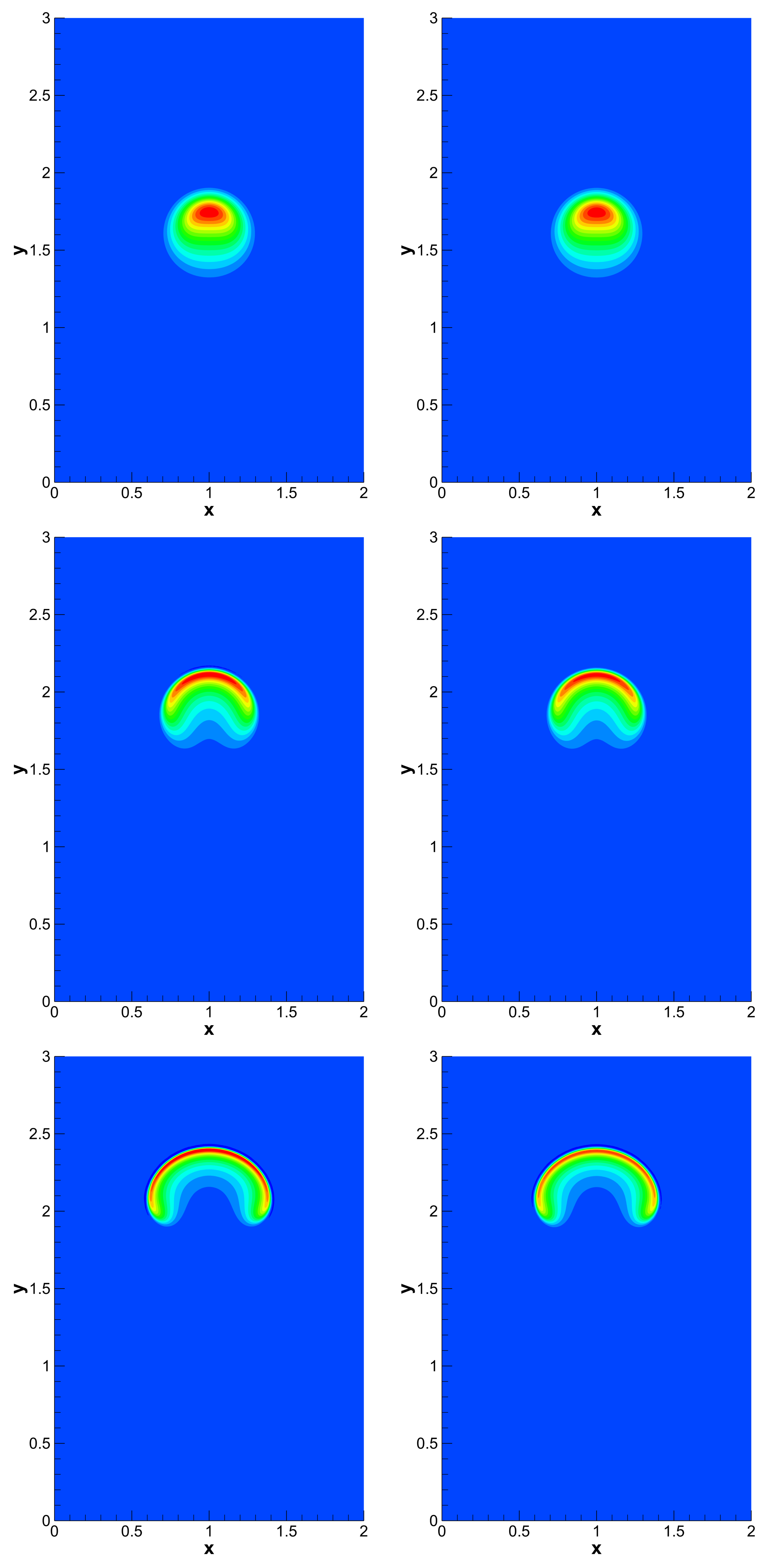
Figure 15.
Comparison of the temperature field obtained using the weakly compressible scheme (left) and the all Mach number solver. From top to bottom: , , .
Figure 15.
Comparison of the temperature field obtained using the weakly compressible scheme (left) and the all Mach number solver. From top to bottom: , , .
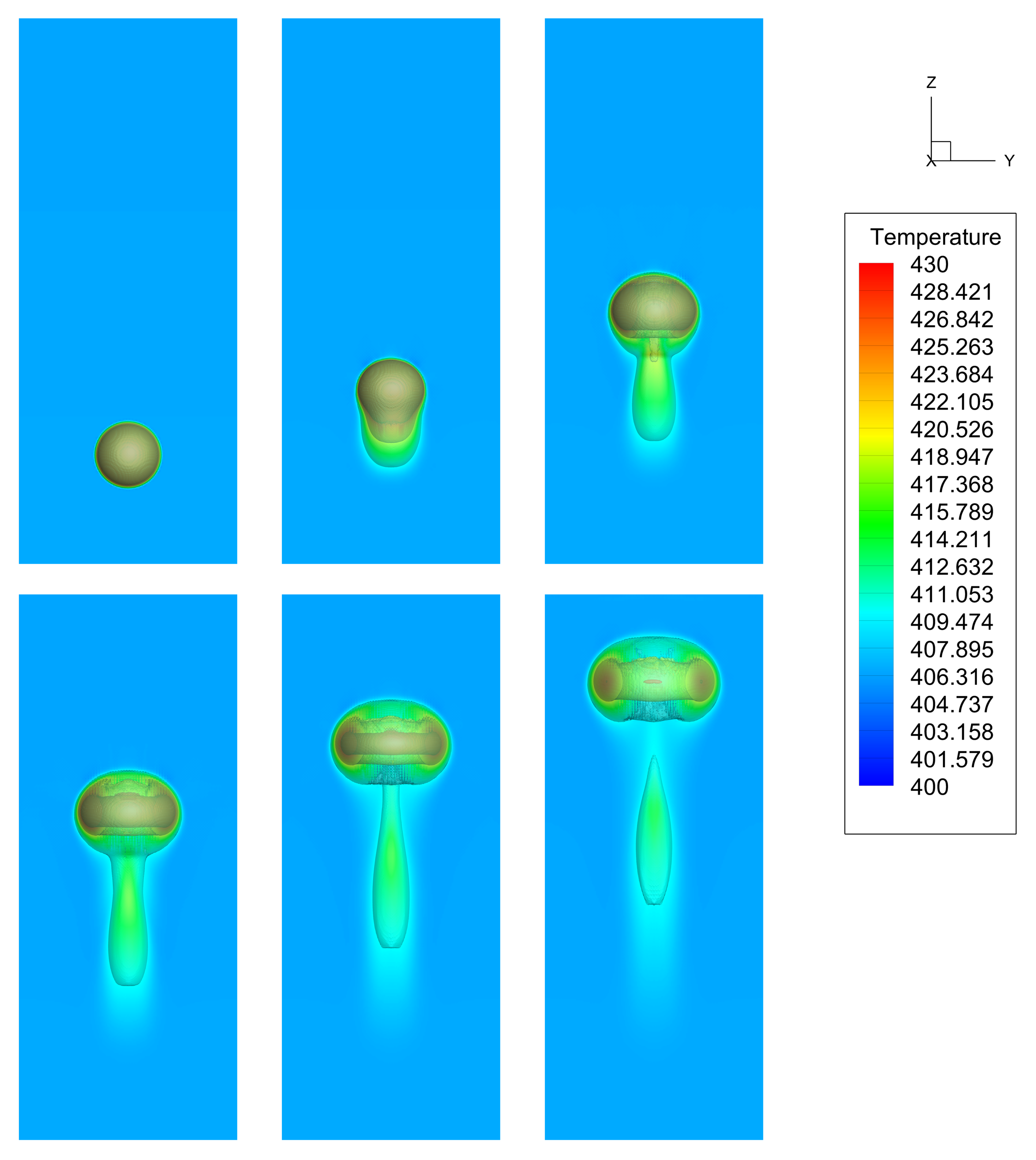
Figure 16.
Temperature contours at plane and isosurfaces for the 3D rising bubble. From top left to bottom right: , , , , , .
Figure 16.
Temperature contours at plane and isosurfaces for the 3D rising bubble. From top left to bottom right: , , , , , .
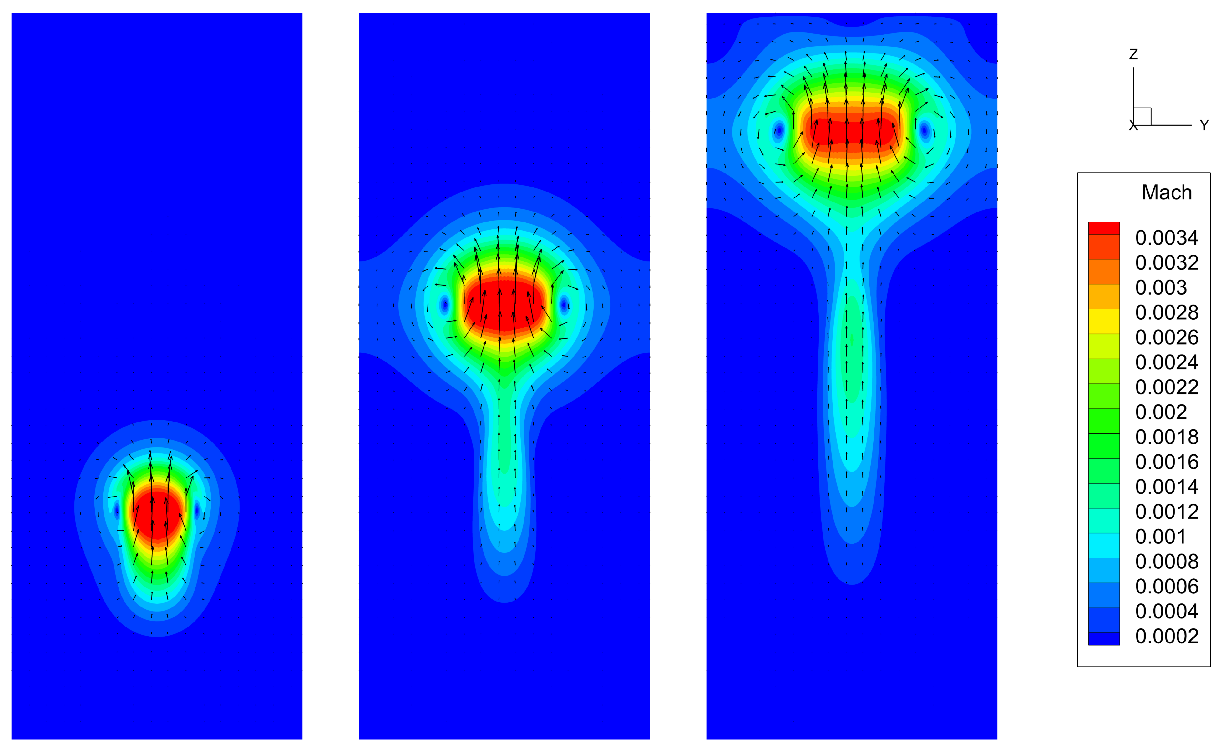
Figure 17.
Mach contours and velocity vectors at plane for the 3D rising bubble. From left to right: , , .
Figure 17.
Mach contours and velocity vectors at plane for the 3D rising bubble. From left to right: , , .
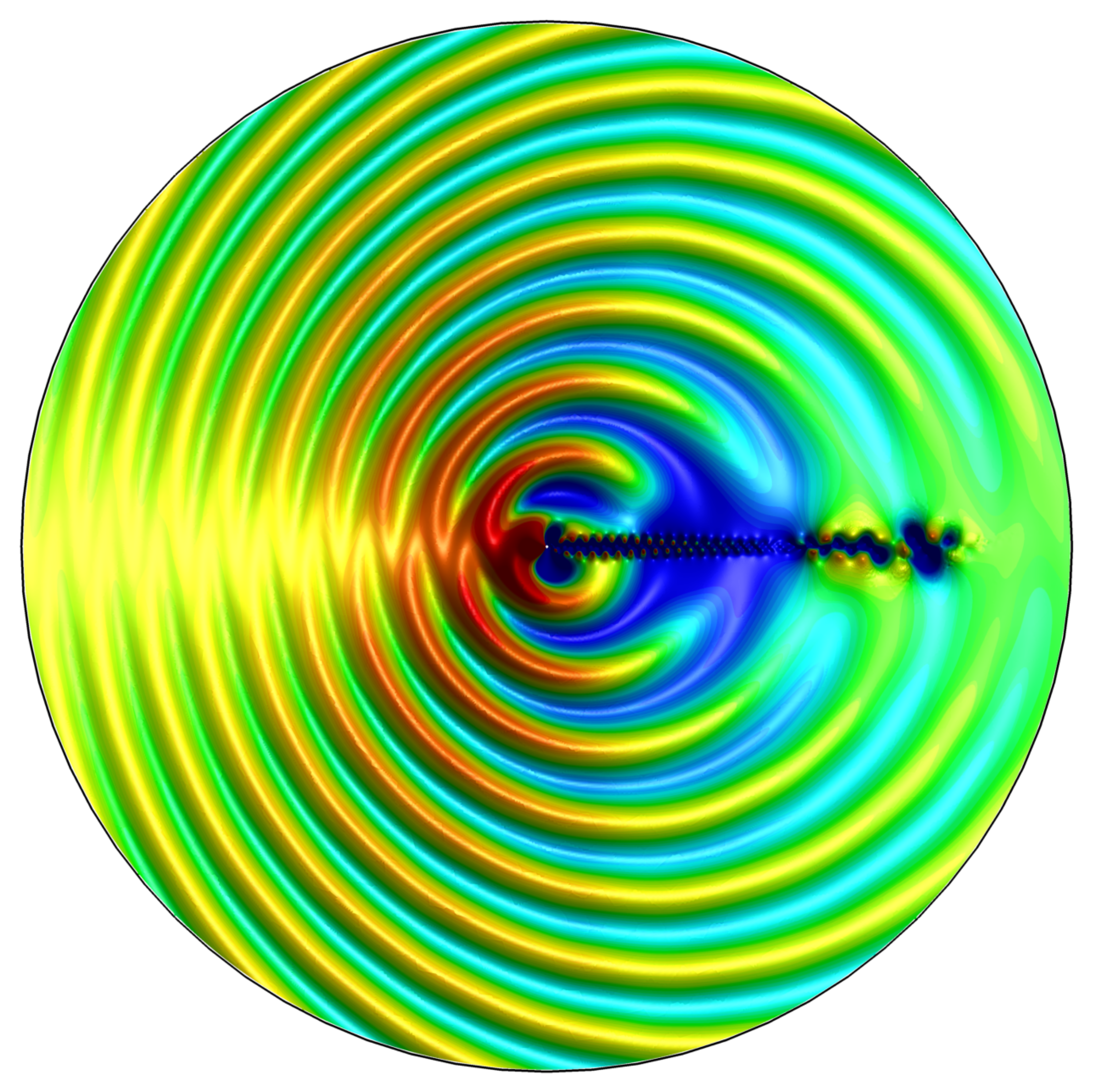
Figure 18.
Sound field generated by the weakly compressible flow around a circular cylinder at time .
Figure 18.
Sound field generated by the weakly compressible flow around a circular cylinder at time .
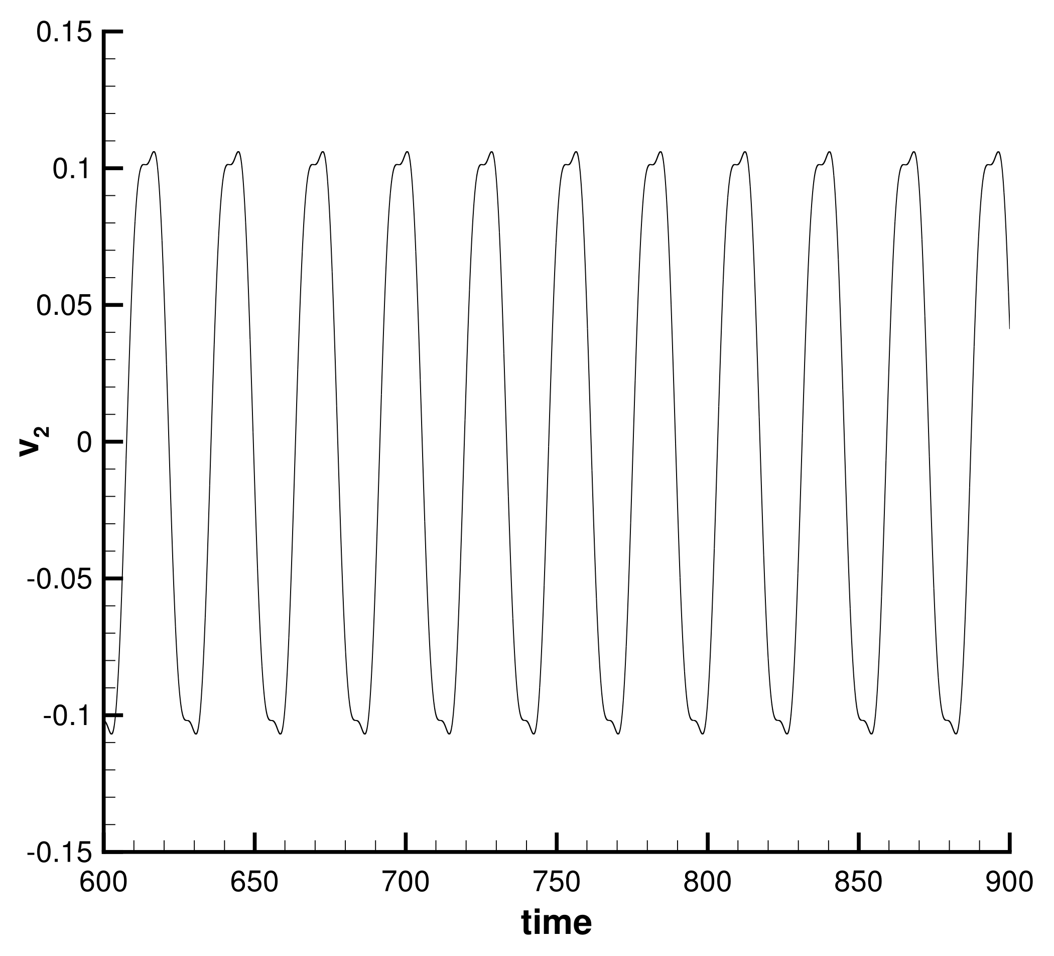
Figure 19.
Time series of the velocity component at in the time interval . The resulting Strouhal number is .
Figure 19.
Time series of the velocity component at in the time interval . The resulting Strouhal number is .
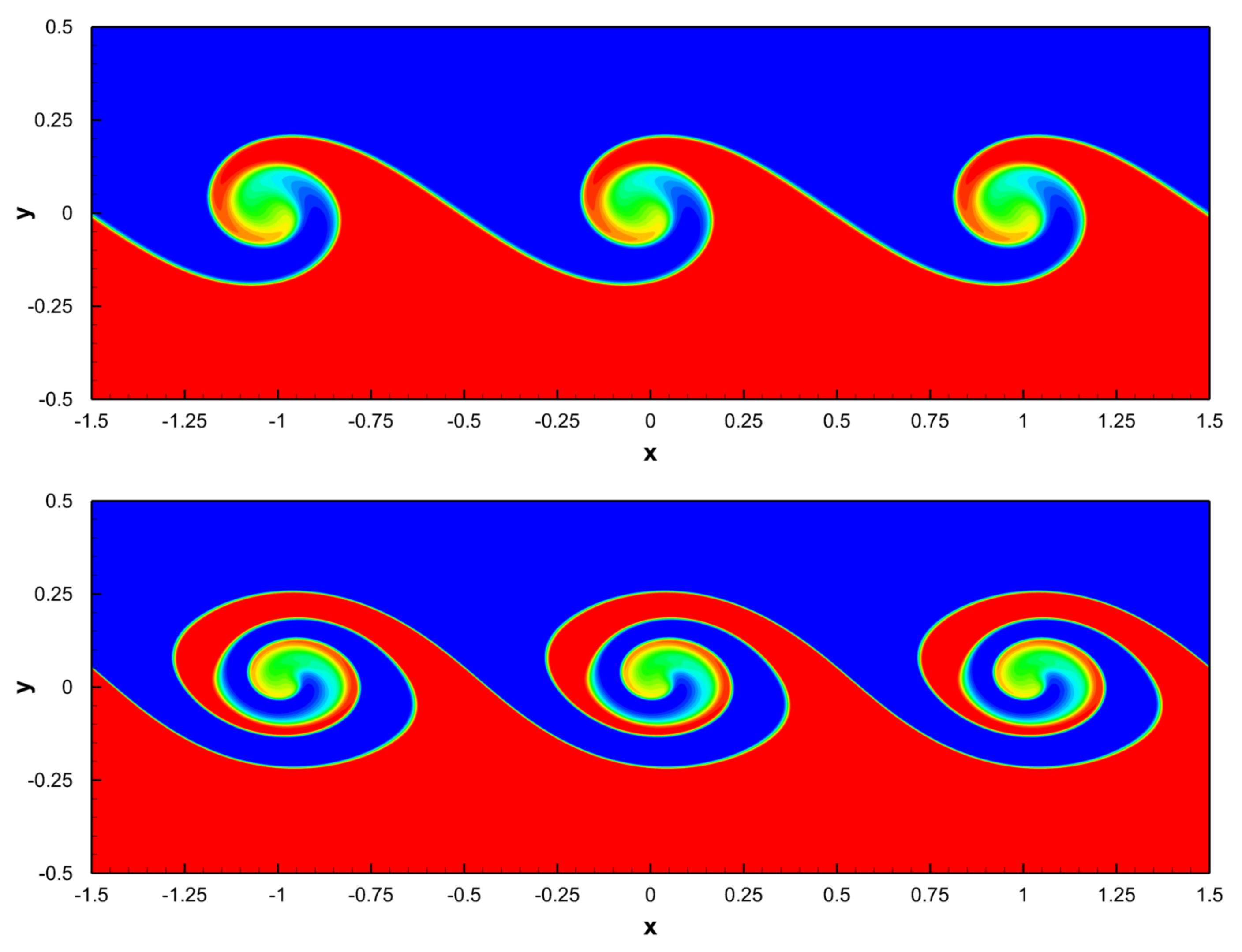
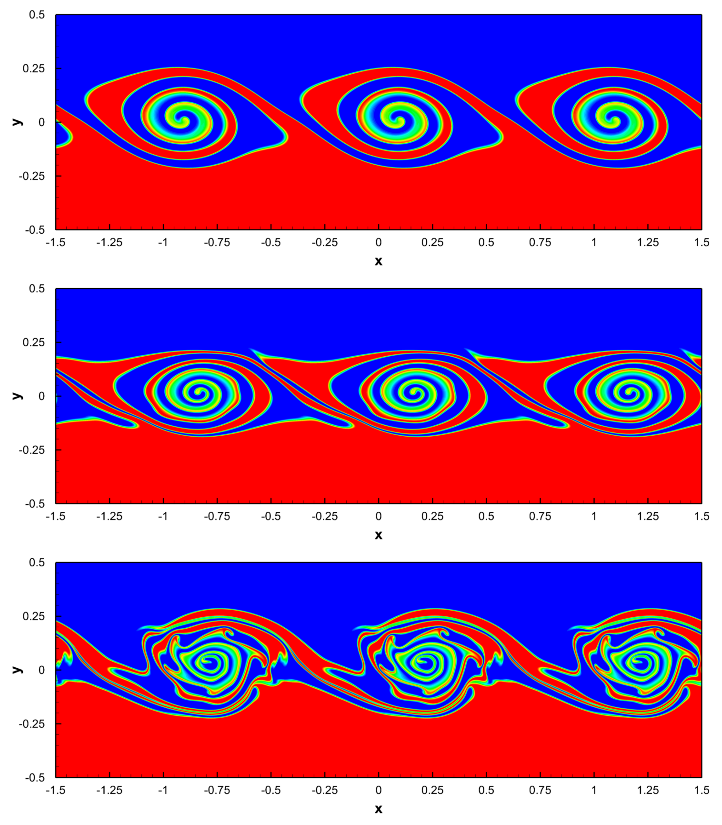
Figure 20.
Temporal evolution of the density contours of the 2D compressible Kelvin–Helmholtz instability at times , , , , , from top to bottom. Three periods of the periodic domain in the direction are shown.
Figure 20.
Temporal evolution of the density contours of the 2D compressible Kelvin–Helmholtz instability at times , , , , , from top to bottom. Three periods of the periodic domain in the direction are shown.
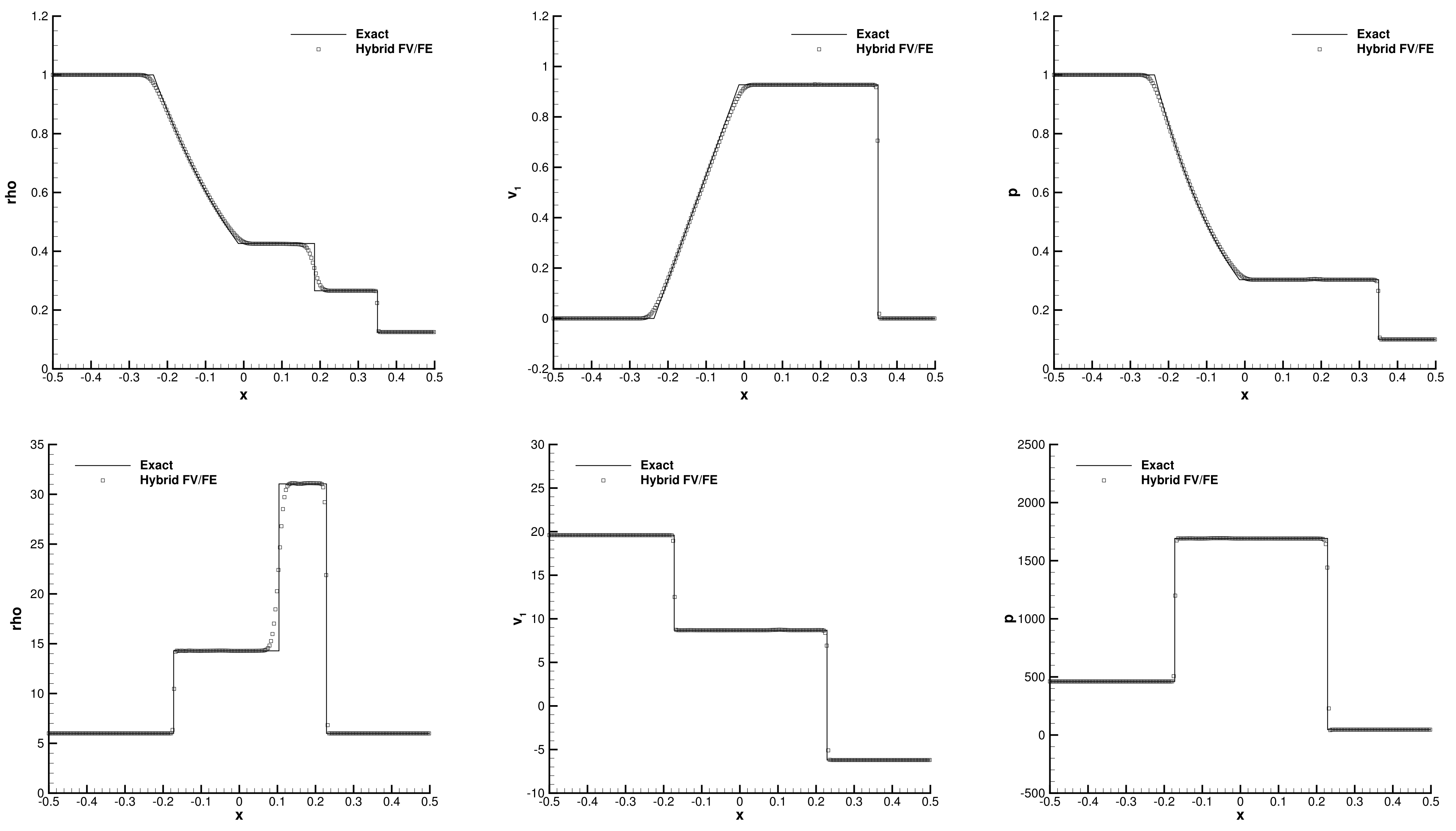
Figure 21.
Riemann problems solved on a regular unstructured 3D mesh composed of primal simplex elements. Top row: results obtained for the Sod shock tube at time . Bottom row: results obtained for the Riemann problem RP4 of Toro at time .
Figure 21.
Riemann problems solved on a regular unstructured 3D mesh composed of primal simplex elements. Top row: results obtained for the Sod shock tube at time . Bottom row: results obtained for the Riemann problem RP4 of Toro at time .
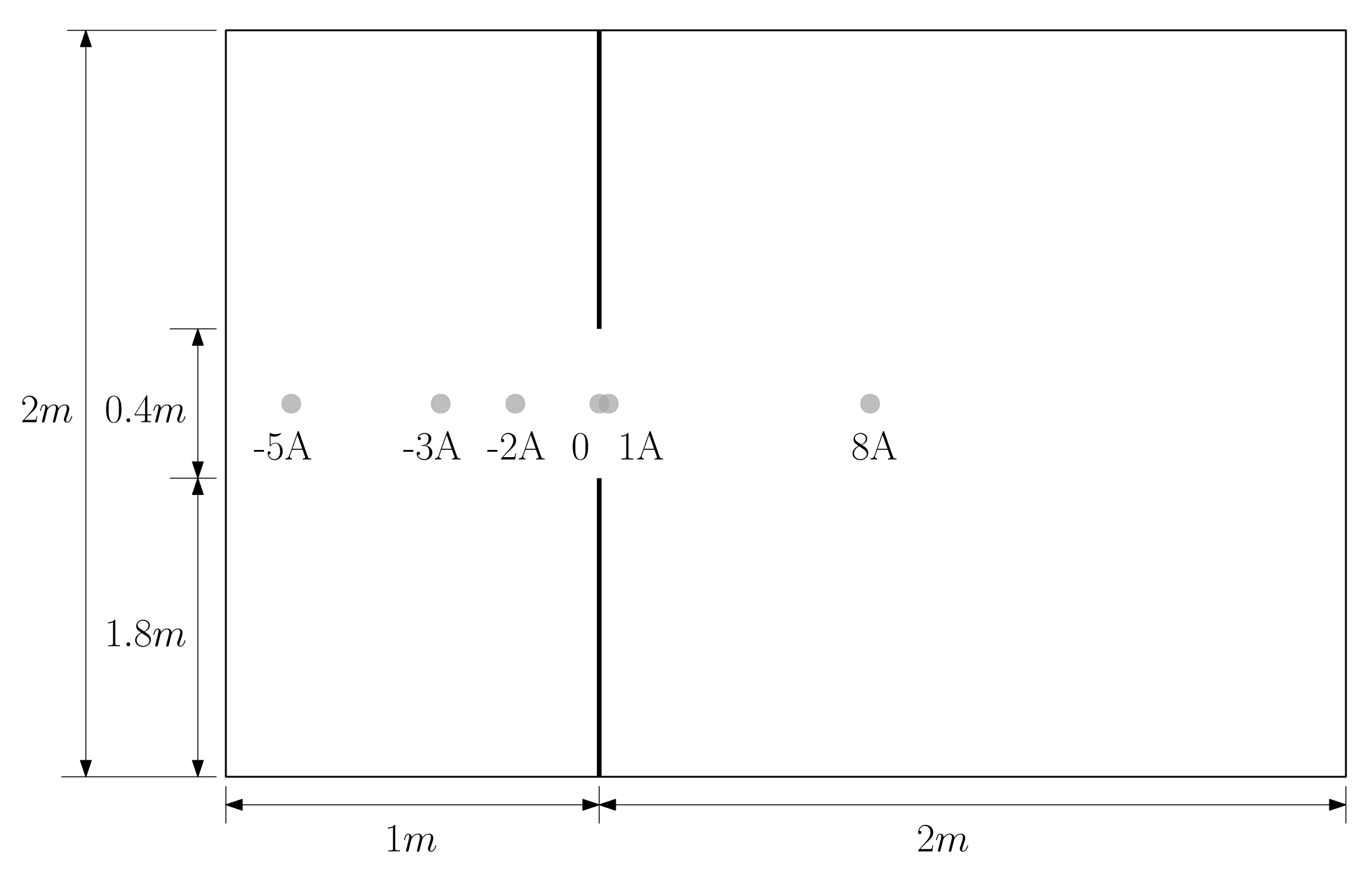
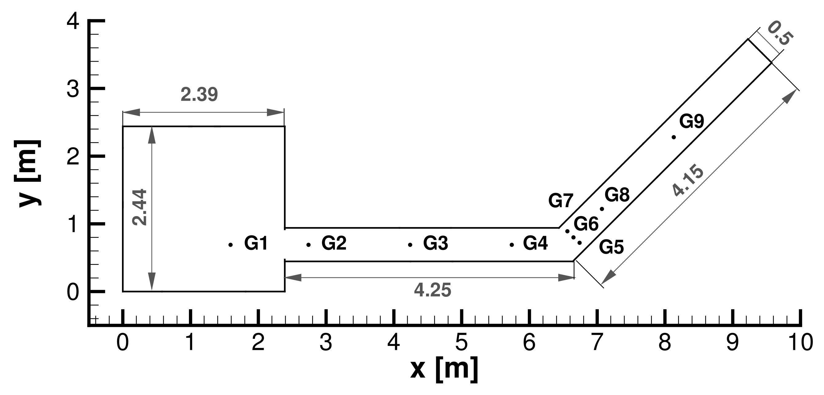
Figure 22.
Sketch of the computational domain for the 3D dambreak on a dry plane test case including the position of the wave gauges.
Figure 22.
Sketch of the computational domain for the 3D dambreak on a dry plane test case including the position of the wave gauges.
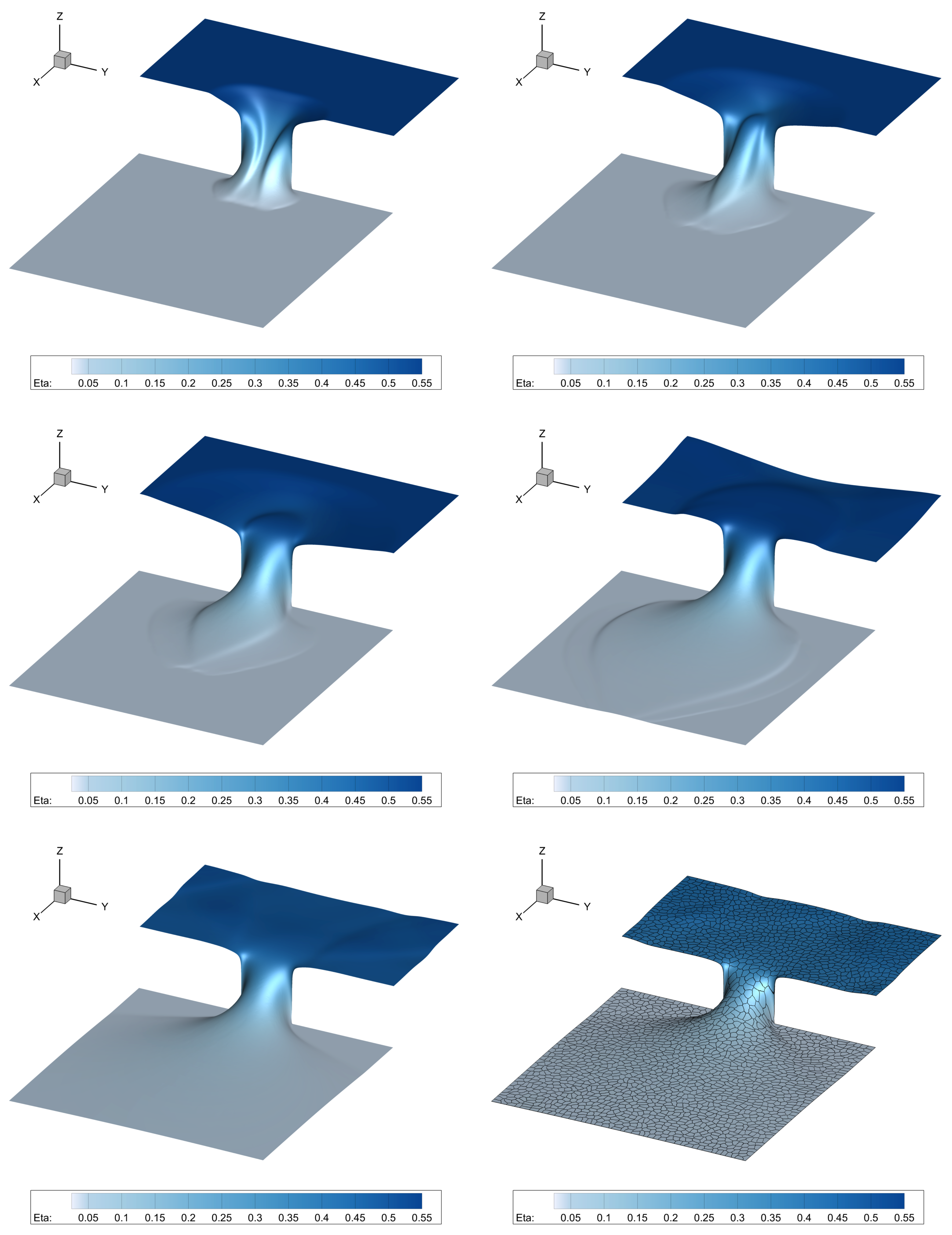
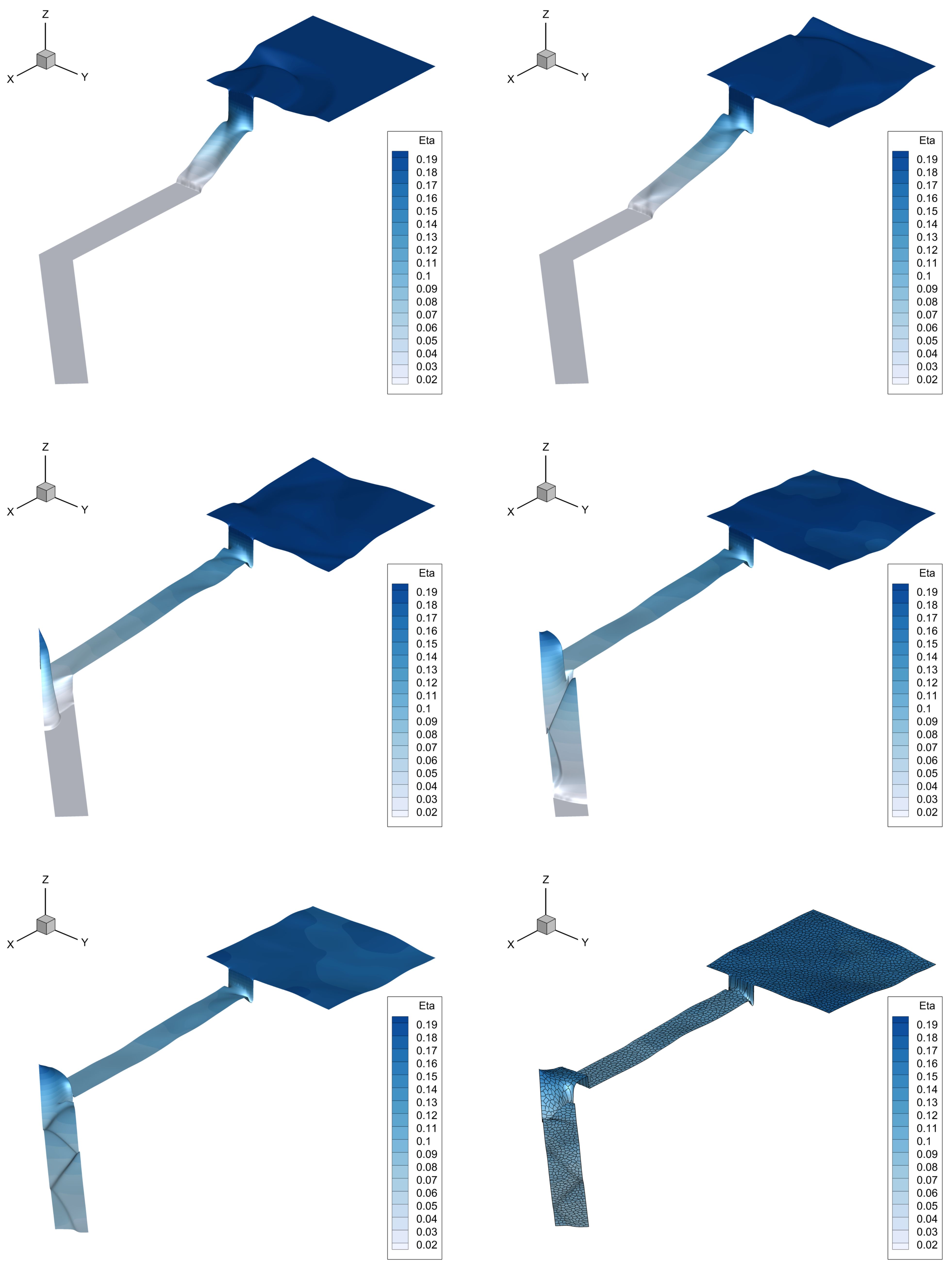
Figure 23.
Water surface for the dambreak over a plane dry bed obtained at times , from top left to bottom right. The last figure also depicts the MPI partition of the computational domain considered to run the simulation on 2400 CPU cores of the SuperMUC-NG supercomputer.
Figure 23.
Water surface for the dambreak over a plane dry bed obtained at times , from top left to bottom right. The last figure also depicts the MPI partition of the computational domain considered to run the simulation on 2400 CPU cores of the SuperMUC-NG supercomputer.
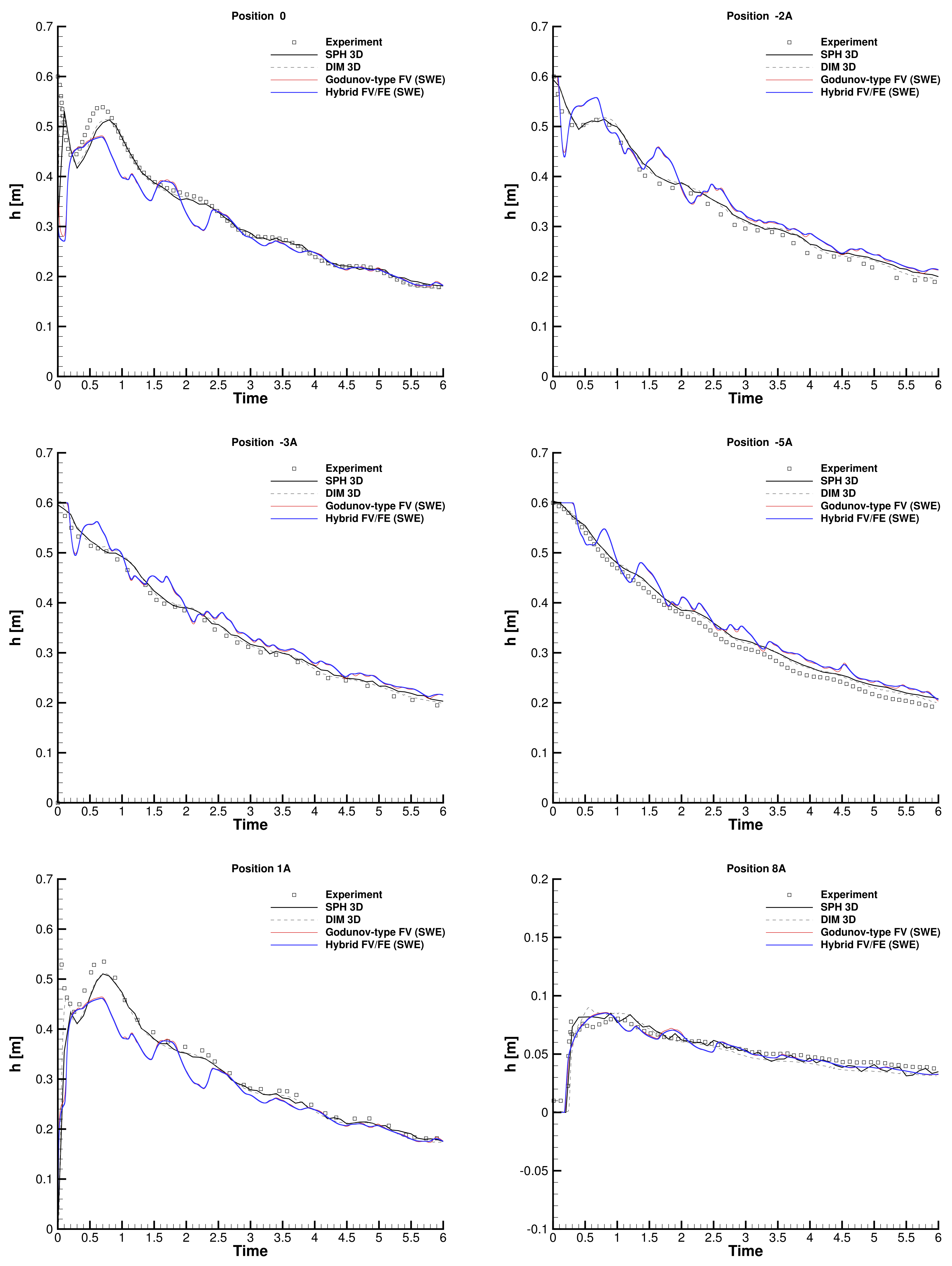
Figure 24.
Time evolution of the free surface elevation obtained at wave gauges 0,
A,
A,
A, 1 A and 8 A for the dambreak over a plane dry bed. Hybrid FV/FE scheme applied to the shallow water equations (blue line); experimental results of Fraccarollo and Toro [
102] (squares); explicit Godunov-type finite volume scheme (red line); fully nonhydrostatic 3D SPH scheme [
103] (black dashed line); 3D diffuse interface method [
104] (black line).
Figure 25.
Computational domain and wave gauges locations for the 3D CADAM test case.
Figure 25.
Computational domain and wave gauges locations for the 3D CADAM test case.
Figure 26.
Free surface elevation of the CADAM test case obtained at times . Right bottom figure also depicts the MPI partition obtained using METIS and used to run the test on 2400 CPU cores of SuperMUC-NG supercomputer.
Figure 26.
Free surface elevation of the CADAM test case obtained at times . Right bottom figure also depicts the MPI partition obtained using METIS and used to run the test on 2400 CPU cores of SuperMUC-NG supercomputer.
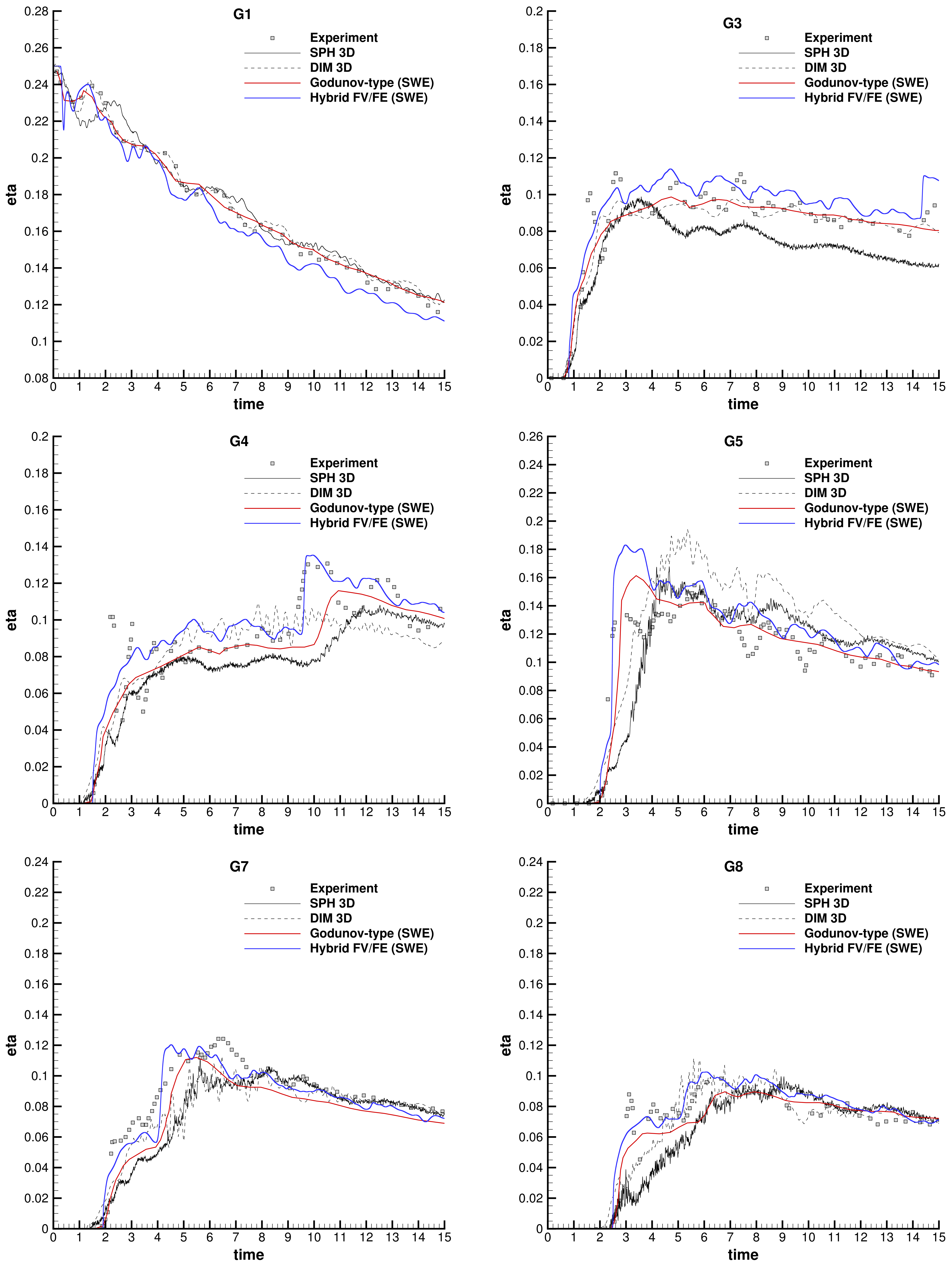
Figure 27.
Time evolution of the free surface at wave gauges G1, G3, G4, G5, G7, G8 (from
left top to
right bottom) for CADAM benchmark. Hybrid FV/FE scheme applied to the shallow water equations run in 2400 CPU cores (blue line); experimental results of Fraccarollo and Toro [
102] (squares); explicit Godunov-type finite volume scheme (red line); fully nonhydrostatic 3D SPH scheme [
106] (black dashed line); 3D diffuse interface method [
104] (black line).
Table 1.
Description of the meshes and time steps used to perform the convergence analysis with the Taylor-Green vortex benchmark in 2D.
Table 1.
Description of the meshes and time steps used to perform the convergence analysis with the Taylor-Green vortex benchmark in 2D.
| Mesh | Elements | Vertices | Dual Elements | |
|---|
| 128 | 81 | 208 | |
| 512 | 289 | 800 | |
| 2048 | 1089 | 3136 | |
| 8192 | 4225 | 12,416 | |
| 32,768 | 16,641 | 49,408 | |
| 131,072 | 66,049 | 197,120 | |
| 524,288 | 263,169 | 787,456 | |
| 2,097,152 | 1,050,625 | 3,147,776 | |
| 8,388,608 | 4,198,401 | 12,587,008 | |
Table 2.
Spatial error norms and convergence rates at time obtained using the LADER scheme for the Taylor-Green vortex benchmark in 2D.
Table 2.
Spatial error norms and convergence rates at time obtained using the LADER scheme for the Taylor-Green vortex benchmark in 2D.
| Mesh | | | | |
|---|
| M1 | 4.13E−01 | | 1.27E−01 | |
| M2 | 1.16E−01 | 1.83 | 3.08E−02 | 2.04 |
| M3 | 2.99E−02 | 1.96 | 7.63E−03 | 2.01 |
| M4 | 7.54E−03 | 1.98 | 1.90E−03 | 2.00 |
| M5 | 1.89E−03 | 1.99 | 4.75E−04 | 2.00 |
| M6 | 4.74E−04 | 2.00 | 1.19E−04 | 2.00 |
| M7 | 1.19E−04 | 2.00 | 2.97E−05 | 2.00 |
| M8 | 2.97E−05 | 2.00 | 7.42E−06 | 2.00 |
| M9 | 7.42E−06 | 2.00 | 1.85E−06 | 2.00 |
Table 3.
Number of spatial divisions and number of MPI subdomains (CPU cores) along each coordinate direction of the grids used for the solution of the three-dimensional Taylor-Green vortex with different Reynolds numbers.
Table 3.
Number of spatial divisions and number of MPI subdomains (CPU cores) along each coordinate direction of the grids used for the solution of the three-dimensional Taylor-Green vortex with different Reynolds numbers.
| Re Number | | |
|---|
| 100 | 128 | 8 |
| 200 | 128 | 8 |
| 400 | 128 | 8 |
| 800 | 256 | 16 |
| 1600 | 512 | 32 |
Table 4.
Initial states left and right, initial position of the discontinuity , and final simulation time t for each Riemann problem.
Table 4.
Initial states left and right, initial position of the discontinuity , and final simulation time t for each Riemann problem.
| Test | | | | | | | | t |
|---|
| RP1 | 1 | | 0 | 0 | 1 | | 0 | |
| RP4 | | | | | | | | |
Table 5.
Coordinates of the wave gauges of the three-dimensional dambreak on a dry plane for a bi-dimensional domain .
Table 5.
Coordinates of the wave gauges of the three-dimensional dambreak on a dry plane for a bi-dimensional domain .
| Wave Gauge | −5 A | −3 A | −2 A | 0 | 1 A | 8 A |
|---|
| x | | | | 0 | | |
| y | 0 | 0 | 0 | 0 | 0 | 0 |
Table 6.
Coordinates of the gauges G1–G8 of the CADAM test case.
Table 6.
Coordinates of the gauges G1–G8 of the CADAM test case.
| Gauge | G1 | G3 | G4 | G5 | G6 | G7 | G8 |
|---|
| x | 1.59 | 4.24 | 5.74 | 6.74 | 6.65 | 6.56 | 7.07 |
| y | 0.69 | 0.69 | 0.69 | 0.72 | 0.80 | 0.89 | 1.22 |


