Abstract
This study was conducted to investigate the applicability of measuring internet traffic as an input of short-term electricity demand forecasts. We believe our study makes a significant contribution to the literature, especially in short-term load prediction techniques, as we found that Internet traffic can be a useful variable in certain models and can increase prediction accuracy when compared to models in which it is not a variable. In addition, we found that the prediction error could be further reduced by applying a new multivariate model called VARX, which added exogenous variables to the univariate model called VAR. The VAR model showed excellent forecasting performance in the univariate model, rather than using the artificial neural network model, which had high prediction accuracy in the previous study.
1. Introduction
As electricity demand grows globally, load demand forecasting has become an important factor in many aspects of energy production and delivery. The time horizons for forecasting are classified as short-, medium-, or long-term. Short-term forecasting (STLF) refers to hourly forecasts, medium-term forecasting (MTLF) for a week to a month, and long-term forecasting (LTLF) for over a year [1]. STLF is mainly used in the operational phase, while LTLF is used in the planning phase. Before information and communication technologies (ICT) and smart grids were developed, forecasting was based primarily on supply-side aggregated data, in top-down formats at large governmental levels. However, owing to recent the development of smart-grid technology, it has become possible to consider end-user demand through a bottom-up approach [2], which can now be applied to STLF. Thus, these technologies have expanded their roles by undertaking the responsibility of forecasting load demand from energy suppliers to consumers.
Summer and winter temperatures are becoming more extreme with rapid climate change, and demand is increasing because of the operation of energy-intensive devices such as air conditioners and heating appliances. In addition, load demand is increasing in buildings and parking lots, because of the surge in electric vehicle (EV) sales [3]. Furthermore, Internet traffic is continuously increasing because of the growing global popularity of smartphones and other Internet communication devices. The Internet makes it possible to find information, send emails, share photos and videos, manage bank accounts, as well as enable access to home network devices remotely. This high demand can also be attributed to the process of traffic delivery and data storage [4].
From a supplier’s point of view, as renewable energy (RE) replaces energy produced from nuclear power, it has become more important to control supply and demand accurately [5]. However, the energy supply uncertainty has become an issue, because RE increases energy supply variability according to factors such as season, temperature, precipitation, cloud cover, and wind speed. The changing pattern of supply and demand has a direct impact on power production, as well as on relative energy prices, power rate settings and government policies. Accurate STLF is therefore an important foundation for the economic, administrative and policy sectors.
Thus, the combination of technology developments, environmental issues, and energy policies for EV, RE, and ICT have made STLF a critical issue in energy markets. Poor STLF can cause energy loss when the demand is overestimated, and blackouts when underestimated, which directly affects economic issues. Therefore, various STLF methods have been studied in recent decades.
Forecasting methods are classified into statistical and non-statistical methods, according to the underlying technique. Statistical methods generate mathematical equations from existing historical data, to estimate model parameters and produce predictions. These methods include autoregressive integrated moving average (ARIMA) models [6,7], Reg-SARIMA-general autoregressive conditional heteroscedasticity (GARCH) models [8], exponential smoothing methods [9], time series models for series exhibiting multiple complex seasonality (TBATS) [10], regression models [11], support vector machine (SVM) models [12,13], fuzzy models [14,15], and Kalman filters [16].
On the other hand, AI-based techniques are known to have high predictive power. They are mainly suitable for nonlinear data because of their nonlinear and nonparametric function characteristics. Many studies using neural network models have been published [17,18]. The recent studies are briefly reviewed here.
For example, Elamin and Fukushige [19] described the SARIMA model with multiple exogenous variables such as temperature, humidity, and monthly, weekly, and hourly dummies. To explain the cross-effects between weather and seasonal factors, combinations of the main effects are considered as interaction variables. Models with interaction terms improved the accuracy of the forecasts.
Sadaei et al. [20] presented a combined method based on the fuzzy time series (FTS) and convolutional neural networks (CNNs) for STLF. The multivariate time series of load demands and temperatures were converted into multi-channel images, and the accuracy of the FTS-CNN model was higher than others.
Al-Musaylh et al. [21] compared multiple data-driven models, such as multivariate adaptive regression spline (MARS), support vector regression (SVR) and ARIMA models, in STLF over forecast horizons. The MARS model showed greater accuracy for 0.5 h and 1.0 h forecasting. However, the SVR model performed better in 24 h forecasting.
Yang and Yang [22] suggested STLF methods for selecting optimal input features (i.e., feature selection, FS) rather than establishing models. Given that the least squares SVM (LSSVM) can solve complex nonlinear problems, a hybrid model combining the auto correlation function FS model and LSSVM regression was applied in STLF.
Singh and Dwivedi [23] implemented a follow-the-leader scheme with a neural network model for STLF, to overcome the problem of overfitting in traditional neural network models. The proposed algorithm was found to outperform the artificial neural network (ANN) and genetic algorithm (ANN-GA), ANN and Jaya algorithm (ANN-Jaya), ANN and PSO algorithm (ANN-PSO), and back propagation neural network (BPNN) models.
Li et al. [24] presented a subsampling strategy for the SVR ensemble forecast method, to improve the accuracy and efficiency in computation. Point estimations were computed, along with confidence levels, to overcome the uncertainty of the forecasts.
Shah et al. [25] attempted to decompose the log demand into deterministic (trend, multiple periodicities) and stochastic parts. To estimate each element from the components of the log transformed data, the autoregressive (AR), non-parametric AR, autoregressive moving average (ARMA), and vector AR (VAR) models were compared. The results showed that the multivariate time series forecasting was superior in accuracy.
Kim et al. [26] comprehensively compared multiple time series (i.e. SARIMA, ARIMA-GARCH and exponential smoothing) and AI-based (i.e.,ANN) methods for STLF over 1 h to 1 day forecasting horizons. It was shown that the optimal model was the ANN model with external variables for weather and holiday effects over the time horizons.
Muzaffar and Afshari [27] studied long short-term memory (LSTM) networks, which are a special type of recurrent neural network, and applied them in learning the long-term dependencies in STLF. Global horizontal, direct normal, and diffused horizontal irradiance, as well as temperature, humidity, and wind speed variables, were considered as potential exogenous variables. Only temperature was applied as a dependent variable, in terms of reducing computational costs. It was shown that LSTM outperforms other methods, such as ARMA, SARIMA, and ARMA with exogenous variables.
Zhu et al. [28] proposed a new weather forecasting technique generated with the dry-bulb temperature profile, relative humidity, and global solar radiation. Then, some of the ranked influential factors were filtered. The final input variables were grouped and applied in an ANN model with back-propagation.
Reddy [29] proposed a Bat algorithm-based back-propagation approach for STLF, with weather factors such as temperature, humidity, and dew point; the best results were obtained in a case study considering temperature and humidity.
J. Morley et al. [30] suggested that understanding Internet traffic usage patterns may lead to simulating the electricity load demand area because Internet networks such as mobile, ICT-related devices, and PCs consume electricity. This phenomenon has become more important as network-based infrastructures grow.
Kim [31] proposed Internet traffic forecasting models using an AR-GARCH error model with seasonal ARIMA models. This motivated our study to build various forecasting models considering Internet traffic data.
As outlined above, some of the common external variables used in these studies include weather and socio-economic variables. As smart grid technology quickly advances, electronic device usage data, as well as non-electronic data, such as meteorological or economic variables, can be easily accessed by region. Many attempts have been made to keep up with the technologies; however, at the time of writing, no clear studies have considered Internet traffic data to forecast load demand. In this study, we have adopted Internet traffic data as an external variable in an ARIMA-based model, and as a dependent variable in a vector AR with exogenous variables (VARX) model. Although the AI-based models are widely used for producing accurate forecast results, it is difficult to discover inference about the variables. Therefore, we demonstrate several representative statistical forecasting methods, and adopt them in a smart grid environment.
The contributions of this paper are presented as follows.
- The existing STLF for load demand is limited to considering only predictor variables such as weather, holidays, and weekends. Thus, we present the effectiveness of considering Internet traffic data as a dependent variable in a multivariate time series forecasting method, and also as an external variable in univariate methods.
- Moving-window prediction techniques were used in STLF to determine which models are superior in the interval k unit from the basic 15 min to 2 h forecasting, and whether the superior models exhibit robustness through these time horizons.
2. Time Series Model
2.1. Taylor’s Double Seasonal Exponential Smoothing Method
Taylor [32] introduced an extended version of the Holt–Winters double seasonal method, to address multiplicative seasonality. This model also assumes that the process of white noise is correlated.
where represents the actual value of demand, represents the seasonal component observed over time (), and and are double seasonal cycles. The components and are the level and trend components of the series at time , respectively. The coefficients , , and are smoothing parameters. is the predicting value of ahead from time .
The initial values are calculated as follows:
The formula of the Taylor’s method is expressed as
where represents the adjusted first-order coefficient, and the smoothing parameters are given by , , , , and .
2.2. Reg-ARIMA-GARCH Model
First, we introduce the basic ARIMA model. The ARIMA model has undergone various developments and was once a benchmark model for time series analysis and forecasting [33]. Once the stationary assumption of the data is confirmed, various time series data are explained with different non-seasonal () orders and seasonal () orders of ARIMA. When series follows ARIMA()() with a mean of , the time series takes the form
where represents the actual value of demand (in kilowatts) observed at time (), and represents the random errors assumed to be white noise during , with a mean of zero and a constant variance of ; and are integers and orders of the model; , where denotes the degree of the non-seasonal autoregressive polynomial; , where is the degree of the non-seasonal moving average polynomial; for the seasonal operators, , where denotes the degree of the seasonal autoregressive polynomial; and , where denotes the degree of the seasonal moving average polynomial. The terms and are the non-seasonal and seasonal difference operators of order and , respectively; is a seasonal cycle.
Next, the external variables are considered to explain the many factors that affect electricity load demand, including holidays, temperature, and socio-economic variables. Typically, climate-related variables are regarded as important factors, imposing high demand on electrical appliances such as heating systems in winter and air conditioning in summer. In this study, temperature, and weekend and holiday indices were included as an explanatory variable in the model.
The Reg-ARIMA model is a regression ARIMA model with error terms [34]. When the series follows the Reg-ARIMA model with number of predictors, the time series takes the form
where is the coefficient of predictors .
The basic ARIMA models can be specifically used under the assumption of constant variance. To adjust the fluctuations of the time series, Engle [35] proposed the autoregressive conditional heteroscedasticity (ARCH) model. Bollerslev [36] extended it as the general ARCH (GARCH) model, whose main feature is that it can handle data with heavier-tailed error distributions. The error term of the ARIMA-GARCH model is defined as
where and are the orders of the GARCH and ARCH processes, respectively; , and are constants; is the error term; is the conditional variance of ; and is a standardized error term.
2.3. VARX Model
Sims [37] introduced the VARX model, a method used to analyze the relationship between multivariate influencing variables. The model is a combination of several AR models, where these models form a vector between the variables affecting each other. The VAR model is a quantitative forecasting approach usually applied to multivariate time-series data.
The VARX() model is defined as
where is a vector of multivariate time-series variables, and is a vector of exogenous variables; and are matrix coefficients; and are and ( column vectors, and and are and matrices, respectively; and is a noise process vector that has a zero mean and is independent during .
3. Data Description and Analysis
3.1. Electricity Load Data
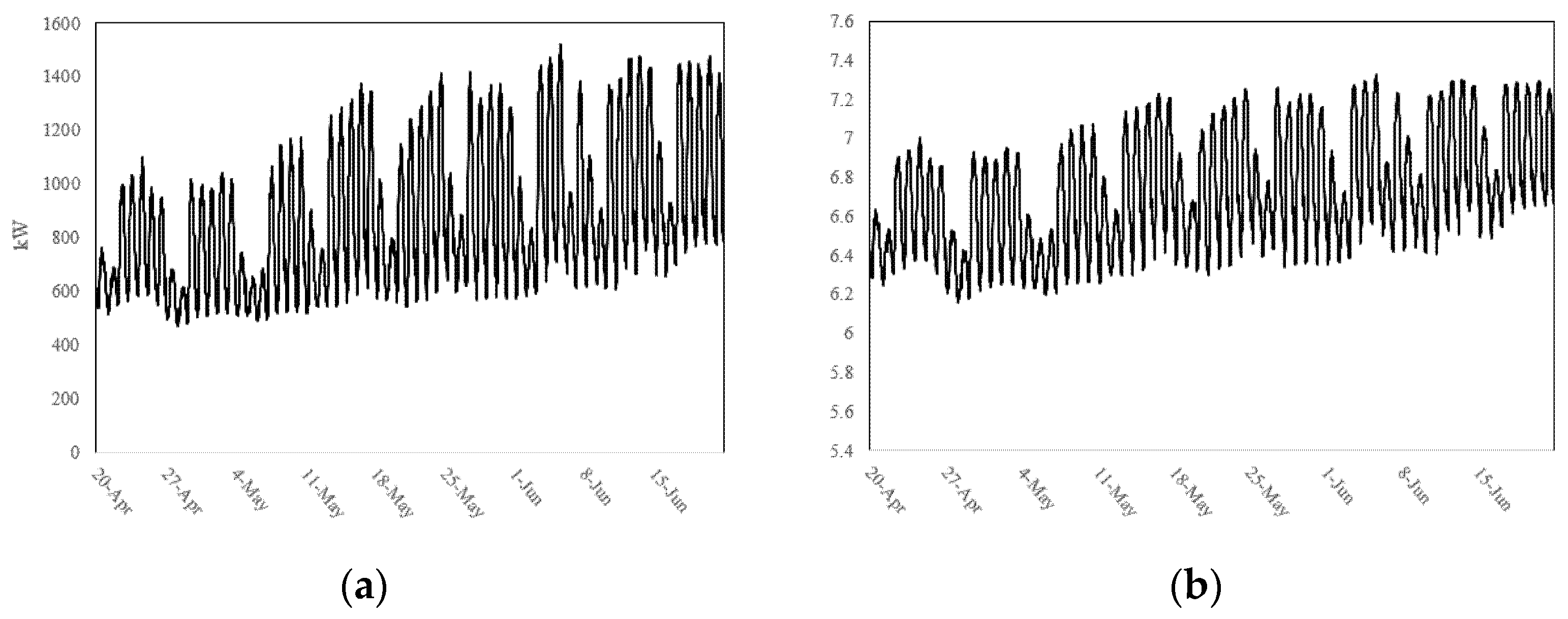
The electricity load data were obtained from Chung-ang University, Seoul, Korea. They were collected at 15 min intervals during the period from 20 April to 21 June 2019. There are a total of 6048 data points. The total floor area of the buildings is approximately 182,730 m2. The campus has 25 buildings comprising research facilities, administrative offices, classrooms, cafeterias, and dormitories. Figure 1a shows a general time series profile of the load data. The electricity load demand shows daily and weekly patterns. It is clear that the Monday through Friday demand is higher than that of the weekend. There is also a decline pattern for the day during national holidays. Figure 1b shows a time-series plot of log-transformed data; it was used as a dependent variable instead of the original series to make an assumption of homoscedasticity in the ARIMA-GARCH models and the VAR model.
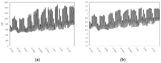
Figure 1.
Electricity load demand plot in (a) Original and (b) Log-transformation.
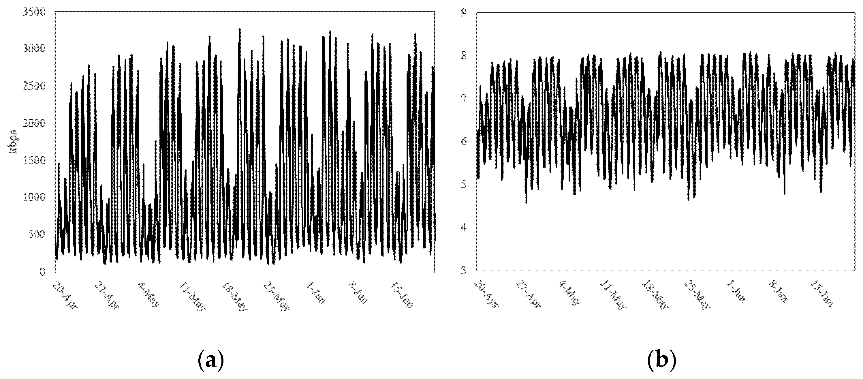
3.2. Internet Traffic Data
The Internet traffic data were obtained from the same campus buildings, over the same period. However, they were collected at 5 min intervals. The data were aggregated into 15 min intervals to ensure comparability to those of the electricity load variable. Figure 2a shows the time series plots of the Internet traffic data. It shows cyclic patterns for the days and weeks, with clearer patterns revealed between weekdays and weekends, compared to Figure 2a. The series was also log-transformed, as shown in Figure 2b. The data were used as an exogenous variable in the Reg-ARIMA-GARCH models, and as a dependent variable in the VAR model.
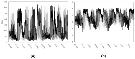
Figure 2.
Internet traffic demand plot in (a) Original and (b) Log-transformation.
3.3. Temperature Data
Weather variables have been widely studied as important variables that may have a great impact on electricity load demand. A positive correlation relationship exists between the temperature and the demand during summer, because of the increased use of air conditioning. However, temperature is also correlated with high demand as temperatures fall during winter, because of the use of heating appliances.
Thus, the relationship between temperature and demand is usually negative in winter, compared to that in summer. Therefore, heating and cooling degree day indices are derived over a half year, to explain such opposite directions of correlation. However, the data used in this study cover April through June (spring in Korea). It was considered that the original temperature data were appropriate for use as an exogenous variable. The data were obtained from the Korea Meteorological Administration as predictor values in the Reg-ARIMA-GARCH models and the VARX model.
3.4. Special Days
To fit the different patterns in demand on weekends and holidays, dummy variables for these days were created. These were applied in the Reg-ARIMA-GARCH models and VARX model, as a predictor variable.
3.5. Data Analysis
The 6048 data observations (9 weeks) were divided into 7 weeks of training data, with the rest for validation. In this study, moving window forecasting methods were considered, and the optimal number of parameters, at each k step, was identified according to the Akaike information criterion for the ARIMA-based models, and to the Schwarz criterion (SC) for the VAR model. Thus, the models are recursively updated to forecast at each training set. Table 1, Table 2, Table 3 and Table 4 represent the examples of estimated parameters and the results for assumptions in the training set.

Table 1.
Parameter estimations of Taylor’s adjusted double seasonal exponential smoothing model.
Table 2.
Parameter estimations of the model.
Table 3.
Parameter estimations of the model with temperature, weekend, and holiday variables.
Table 4.
Parameter estimations of the model with temperature, weekend, holiday, and Internet traffic variables.
Table 1 indicates the estimated coefficients for Taylor’s double seasonal exponential smoothing method. We took the double seasonal cycles to describe a day () and a week ().
The residuals from ARIMA-fitted values were checked to see if there was a heteroscedasticity in the case of basic ARIMA models: (1) without any predictor variables; (2) with temperature and special-day variables and (3) with temperature, special-day, and Internet traffic variables. Although the Ljung-Box Q-statistics show that the standardized residuals were insignificant for the ARIMA models (1) p = 0.5735, (2) p = 0.5551, (3) p = 0.7010), it was shown that there is heteroscedasticity from the same results on the squared standardized residuals (1) p < 0.0001, (2) p < 0.0001, (3) p < 0.0001). To ensure that there are ARCH effects in the model, Engle’s Lagrange multiplier tests were additionally conducted. The tests proved that the volatilities need to be fitted by the GARCH term in the ARIMA-based models.
Table 2, Table 3 and Table 4 show the estimated coefficients from the ARIMA-GARCH model for the same cases as the ARIMA models. Here we can interpret how much each exogenous variable impacts the demand by coefficients. For example, Table 4 shows that more demand was observed as temperature or Internet traffic increased. On the other hand, less demand was observed on weekends and holidays.
Rather than considering the Internet traffic data as one of the input variables in the models, we tried to forecast the electricity load demand and the Internet traffic demand using the VAR model. Before fitting the model, the augmented Dickey–Fuller (ADF) test was conducted to determine if the main dependent variables had a unit root. The log-transformed series datasets were used for the test, setting trends and intercepts in both series. The optimal lag length was automatically selected based on the SC. Given that Table 5 indicates that those two series were stationary, there is no need to perform a further Johansen’s cointegration test. To clarify the stationary assumption, the ADF test for the series, with the option having intercepts without trends, was conducted. In addition, the null hypothesis of non-stationarity was rejected in both series. Therefore, the VARX model was deemed an appropriate method. Table 6 shows the estimated coefficients matrix from the VAR model with temperature and special-day variables.
Table 5.
Augmented Dickey–Fuller (ADF) test of log-transformed Electricity Load and Internet traffic data.
Table 6.
Parameter estimations of VARX(4,0) model.
4. Performance Evaluations
This section discusses comparisons of the various models performed using mean-absolute-percentage-error (MAPE) and root-mean-square error (RMSE). These evaluation methods are widely used to evaluate model performance, especially for STLF.
MAPE is defined as
where is the actual value and is the forecasted demand at time . The equation of RMSE is given by
Here we also obtained the accuracy results of the Internet traffic from the VAR model, but given that the main purpose of our study is to forecast electricity load demand, we only discuss the results of the power demand. Table 7 presents the MAPE results in the validation set at k steps ahead. It shows that the VARX model is superior to other models, through all steps. The second-best model was the ARIMA-GARCH model (3), with temperature, special-day, and Internet traffic variables; it showed higher accuracy than the other ARIMA-GARCH models that did not consider Internet traffic values as an input.
Table 7.
Forecast performance evaluation by MAPE.
Table 8 shows the validation RMSE values; the performance of the VARX and GARCH-based models showed the same patterns as those for the MAPE. However, in the case of comparing the exponential smoothing method to ARIMA model (1), without any predictor variables, the ARIMA model showed better performance than that of the Taylor’s model. That is, it is preferred to fit ARIMA models for univariate datasets.
Table 8.
Forecast performance evaluation by RMSE.
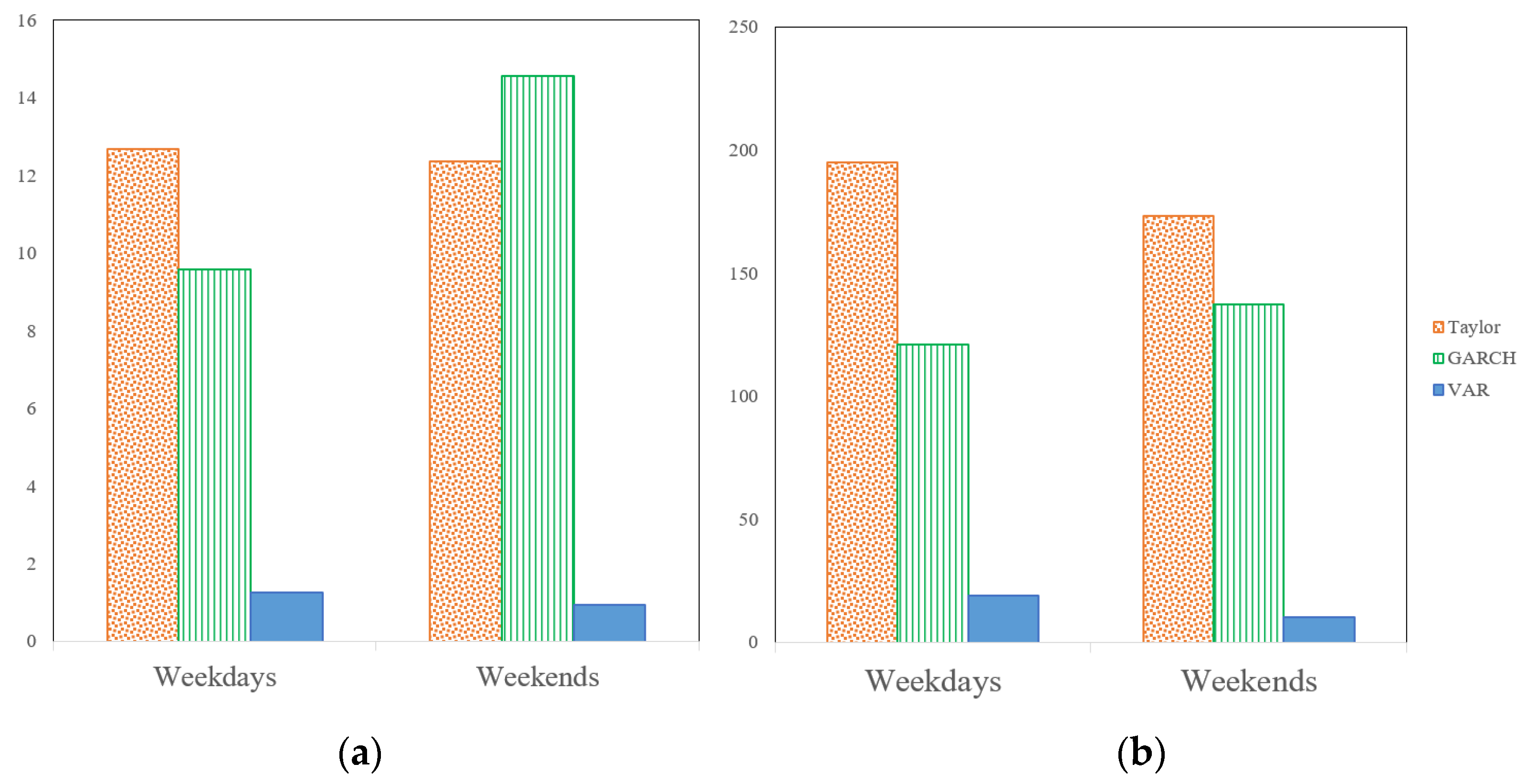
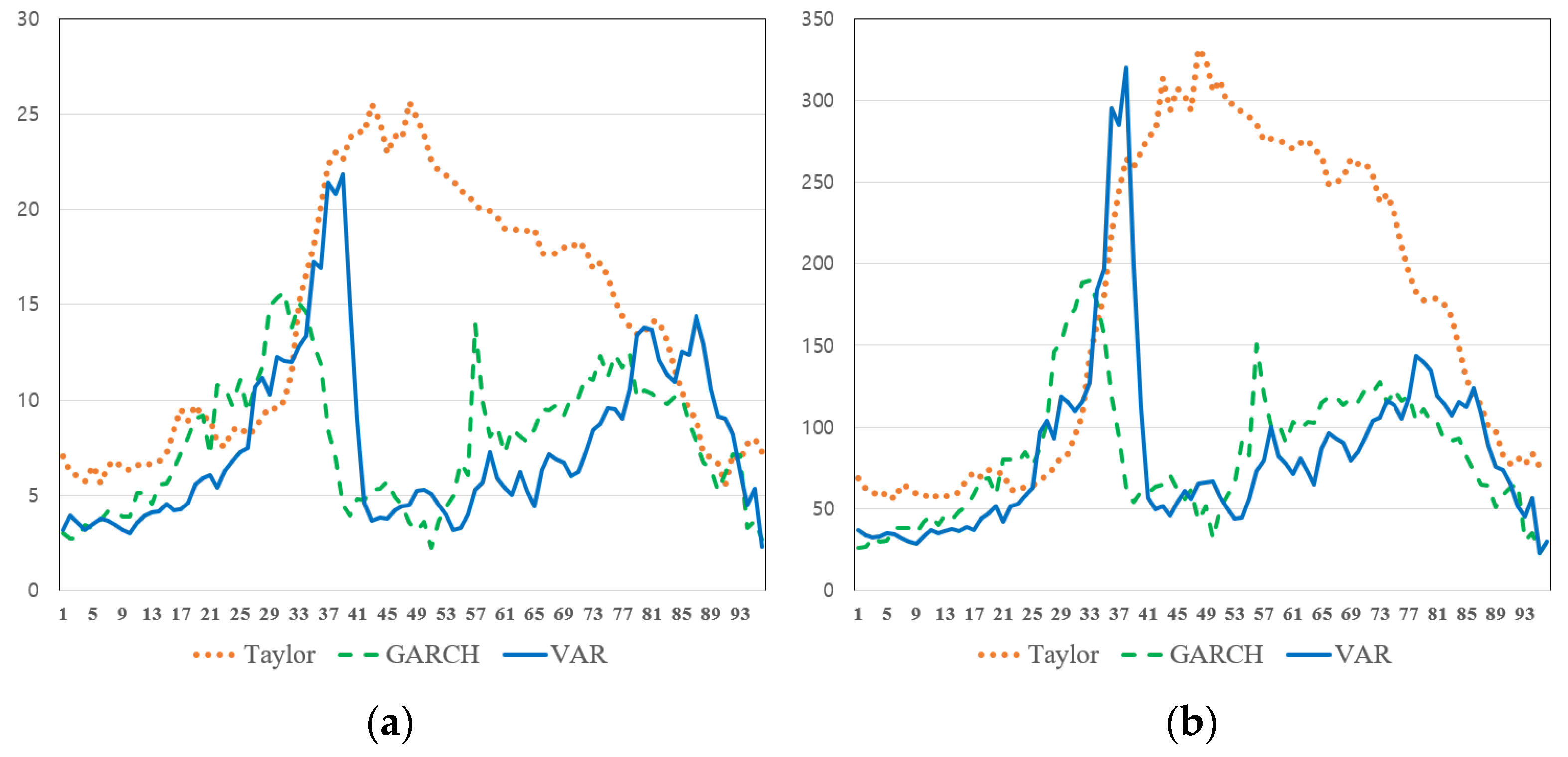
Figure 3, Figure 4, Figure 5 and Figure 6 show graphical model performances stratified by day type (Figure 3 and Figure 4) and quarter-hour (Figure 5 and Figure 6) for the MAPE and RMSE for 1 h and 8 h forecasts, respectively. Here, we only compare three representative models: Taylor’s exponential smoothing method, ARIMA-GARCH 3, and VARX models; and we assume four variables were available: temperature, special day, Internet traffic, and Electricity load demand.
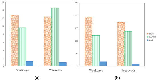
Figure 3.
Forecast (k = 1) performance evaluations categorized by day type for models in terms of (a) MAPE and (b) RMSE.
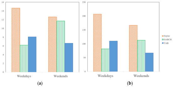
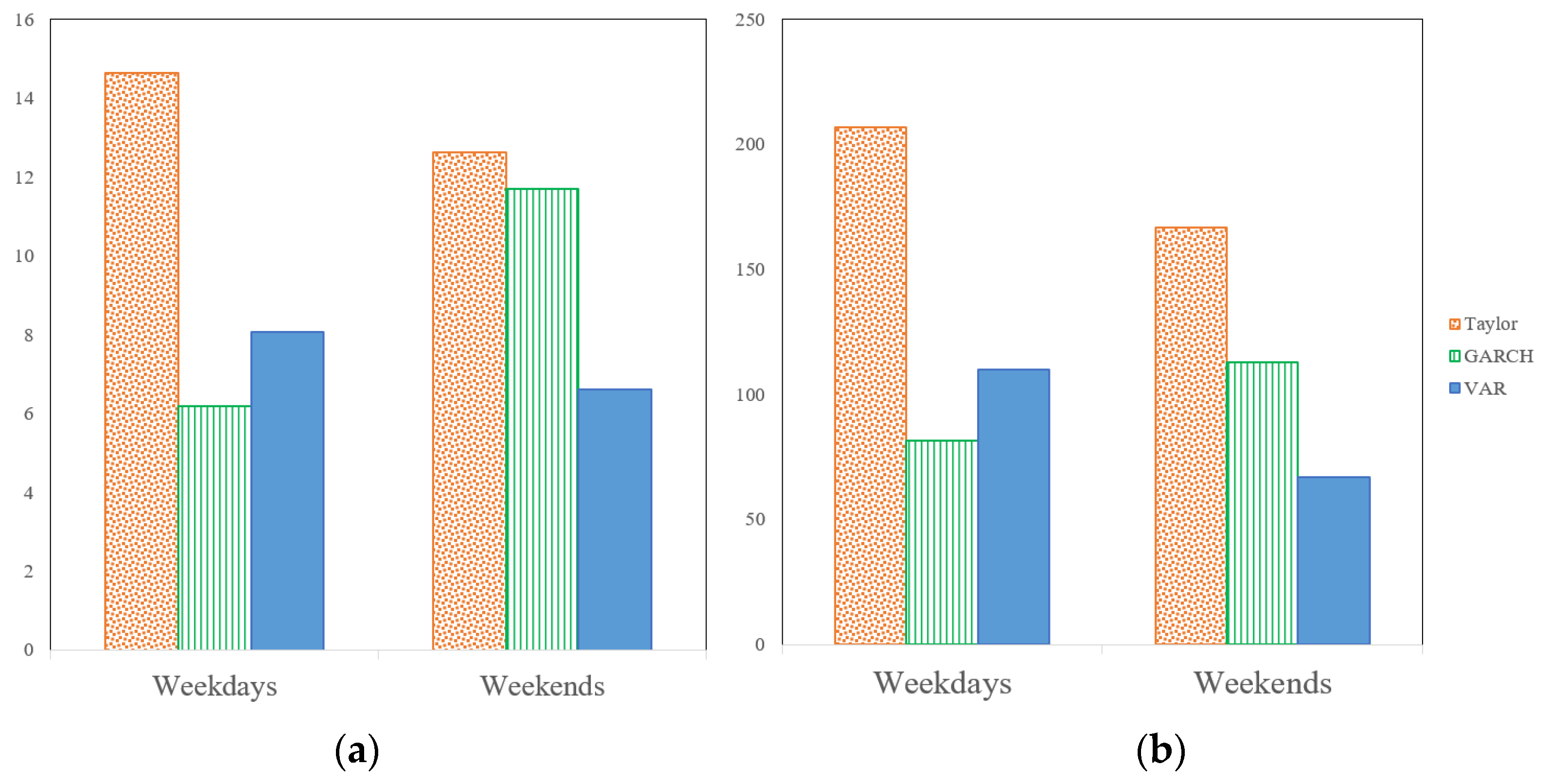
Figure 4.
Forecast (k = 8) performance evaluations categorized by day type for models in terms of (a) MAPE and (b) RMSE.
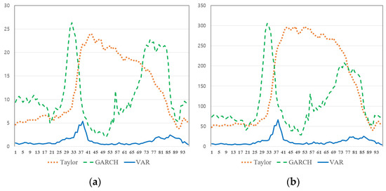
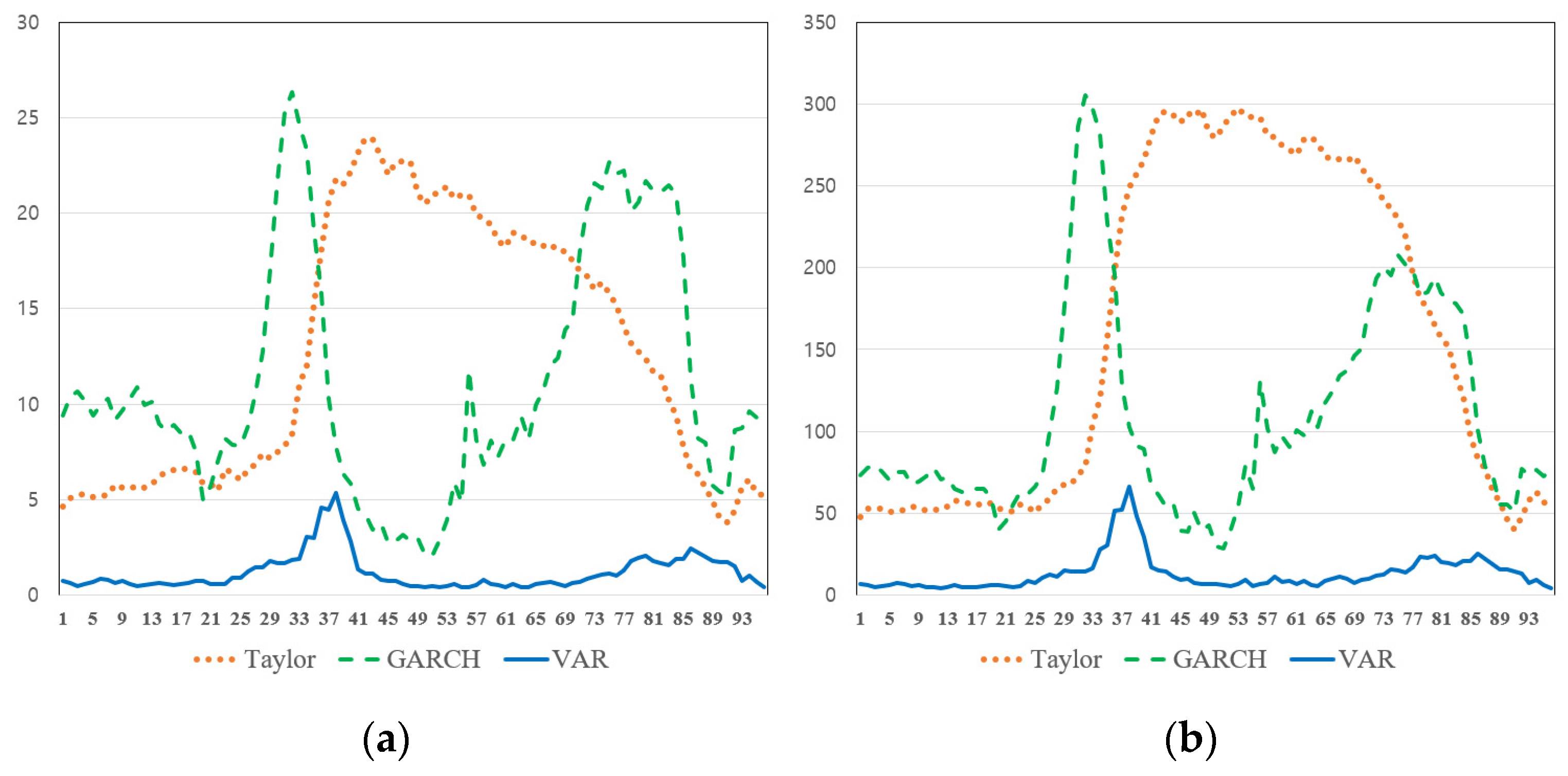
Figure 5.
Forecast (k = 1) performance evaluations categorized by quarter-hour for models in terms of (a) MAPE and (b) RMSE.
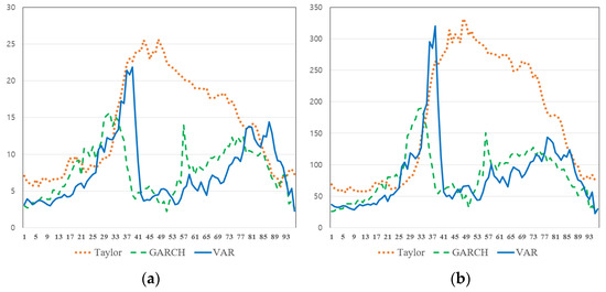
Figure 6.
Forecast (k = 8) performance evaluations categorized by quarter-hour for models in terms of (a) MAPE and (b) RMSE.
Figure 3 represents accuracy plots categorized by day type for 15 min forecasting. Special days were excluded in the day type stratification because there were no holiday seasons in the test set period. The VAR model shows the lowest error regardless of the day type, in terms of MAPE and RMSE. However, forecasts on weekdays were less accurate in ARIMA and VAR models, while the GARCH model shows the opposite.
Figure 4 shows the accuracy plots by day type for 2 h forecasting. It shows similar patterns to that of the 15 min forecasting, but the VAR model show less accuracy in weekday results. If the forecasting horizons are very short (k = 1), then the VAR model should be suggested. However, if the horizons are short (k = 8), the ARIMA-GARCH model is worth consideration.
Figure 5 shows accuracy plots categorized by quarter-hour forecasting. Notably, the x-axis sequence of 1 to 96 corresponds to 00:15 a.m. to midnight. Forecasts prove less accurate between 9:00 a.m. to 10:45 a.m. (x = 32–39) when the morning classes begin. Although the GARCH and VAR models show better performances in the afternoon, the ARIMA model shows continuously poor results until night. The VAR model outperforms during general hours, but the accuracies of the GARCH model diminishes again between 07:00 p.m. to 10:30 p.m. (x = 72–86).
Figure 6 shows the accuracy plots for 2 h forecasting. The ARIMA and GARCH models show similar patterns to the 15 min forecasting. However, the performance of the VAR model is poor as it is best suited to very short-term forecasting. As seen in Figure 4, the ARIMA-GARCH model provides higher accuracy than the VAR model.
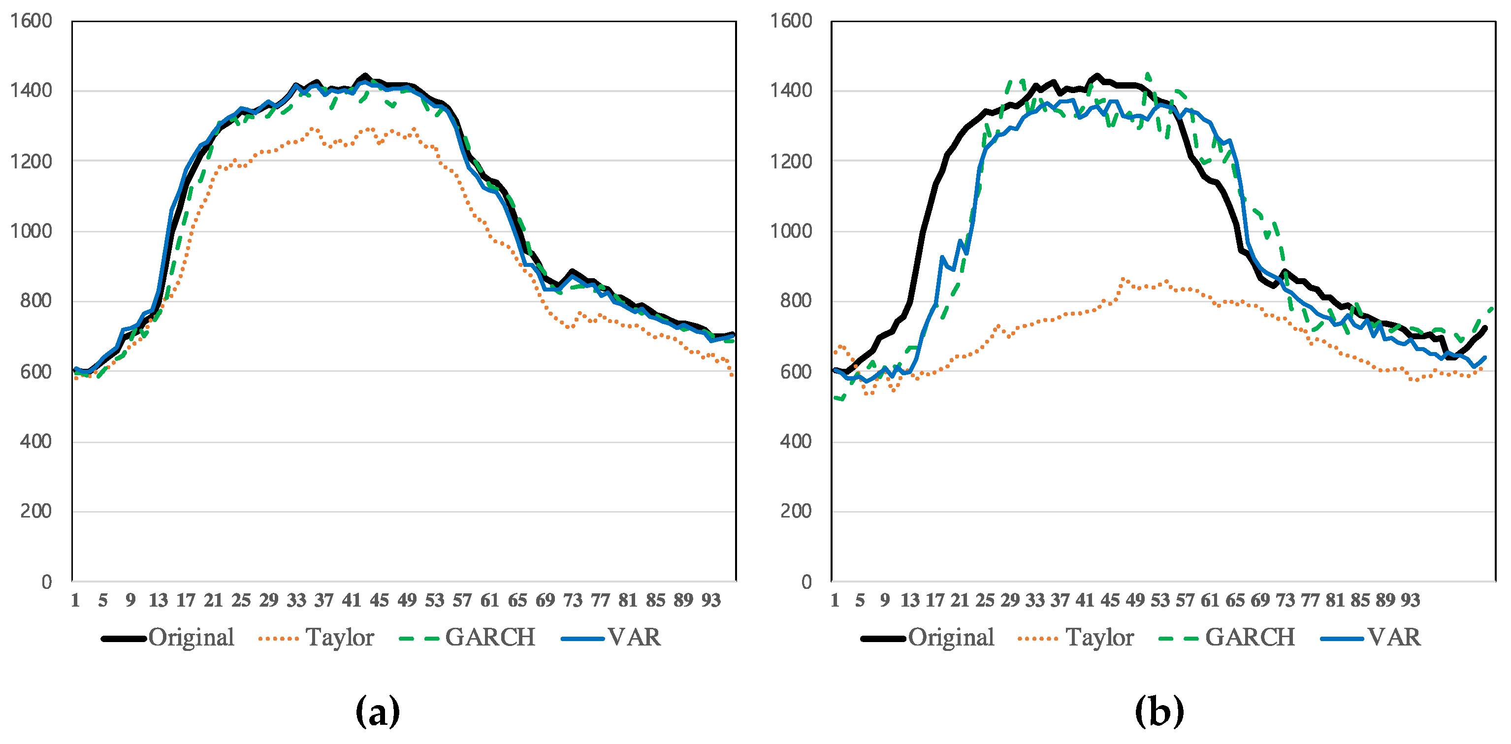
Figure 7 represents the actual values of the day after the national holiday from the validation set to compare the predicted values from each model. The 15 min (k = 1) forecasting does not show much difference in general, but Taylor’s model showed underestimated in terms of level. The 2 h (k = 8) forecasting also shows that Taylor’s model significantly underestimates predicted values above the others. We assume the main reason for this is the fact that Taylor’s model cannot apply the exogenous variables such as a special day.
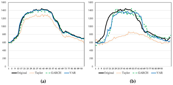
Figure 7.
Comparison between the original values and each model from (a) forecast (k = 1) and (b) forecast (k = 8).
5. Concluding Remarks
Accurate STLF is a critical issue for decision makers and power generation companies in terms of policy making and development planning. Thus, many attempts have been made to improve the performance of electricity load prediction. This study examined the relevant time series methods for short-term forecasting of electricity load demand through 15 min to 2 h time horizons, in an institutional campus in Seoul. Taylor’s double seasonal exponential smoothing methods, ARIMA-GARCH models, and the VARX model were used for optimization. In this study, these models provided the lowest MAPEs and RMSEs from 15 min (k = 1) to 2 h (k = 8) forecasting.
The results show that the VAR model is superior to the other univariate models through all steps. Taking the indirect variable as another dependent variable, rather than applying it as input values, provided high accuracy as well as the advantage of time efficiency, with a multivariate model. However, caution must be applied when using the VAR model, by checking the series are stationary and if not, a further cointegration test is required. Sometimes the cointegrated relationship shows up in the same variables with longer data sets, with lower frequency. If this is the case, the vector error correction model is considered the appropriate method. It is known that sometimes it shows strong evidence in the relationship between multivariate variables, depending on the length, or time, unit of the datasets.
The second-best model was the ARIMA-GARCH with Internet traffic, temperature and special-day predictors. It demonstrated that Internet traffic data are useful as input values, even in univariate models. The results were not always good when fitting volatilities, with the GARCH term in the ARIMA models through all steps, even though the ARCH effects tests indicated heteroscedasticity in the data. However, the data in this study were appropriate for STLF, by fitting GARCH models including the Internet traffic usage data.
In buildings that do not offer Internet traffic data, it is worth considering finding a potential dependent variable in a multivariate model such as VARX.
The results demonstrated that weather and holiday characteristics have an impact in demand forecasting. However, even if the external variables were appropriate, the accuracy varies, depending on whether the model fits the volatilities in the data. Although the best-fitted model was the VARX model using electricity load demand and Internet traffic data as multiple dependent variables, the other models still offer great insights for considering explanatory factors. In addition, using the VARX model is fast and time-effective.
Further, we discuss the model performances in depth by stratifying day types and quarter-hour of the days, to compare ARIMA, ARIMA-GARCH, and VAR models with exogenous variables. We show that the forecasts degrade over the time horizon, and the VARX model is not universally superior to other models.
In this study, we mainly aimed to compare the performance of the exponential smoothing methods, ARIMA-GARCH models, and VARX models. However, different adaptations of the models, such as SVM models, fuzzy models, and Kalman filters will be examined in future study.
Other future studies may set the goal of building an optimal and customized forecasting model for each single unit/building, according to building size, age, and type of external wall (for smaller units).
Author Contributions
Conceptualization, S.K. and Y.K.; methodology, S.K. and Y.K.; software, Y.K.; validation, S.K.; formal analysis S.K. and Y.K.; writing—original draft preparation, Y.K.; writing—review and editing, S.K.; visualization, Y.K.; supervision, S.K.; project administration, S.K.; funding acquisition, S.K. Both authors have read and agreed to the published version of the manuscript.
Funding
This research was funded by Korea Institute of Energy Technology Evaluation and Planning (grant number 20199710100060), and the National Research Foundation of Korea (grant number 2016R1D1A1B01014954).
Institutional Review Board Statement
Not applicable.
Informed Consent Statement
Not applicable.
Data Availability Statement
The data have been collected from Office of Information and Communication Technology, Chung-Ang university.
Conflicts of Interest
The authors declare no conflict of interest. The funders had no role in the design of the study; in the collection, analyses, or interpretation of data; in the writing of the manuscript, or in the decision to publish the results.
References
- Hong, T.; Fan, S. Probabilistic electric load forecasting: A tutorial review. Int. J. Forecast. 2016, 32, 914–938. [Google Scholar] [CrossRef]
- Reyna, J.L.; Chester, M.V. Energy efficiency to reduce residential electricity and natural gas use under climate change. Nat. Commun. 2017, 8, 14916. [Google Scholar] [CrossRef] [PubMed]
- Habib, S.; Kamran, M.; Rashid, U. Impact analysis of vehicle-to-grid technology and charging strategies of electric vehicles on distribution networks–a review. J. Power Sources 2015, 277, 205–214. [Google Scholar] [CrossRef]
- Coroama, V.C.; Hilty, L.M.; Heiri, E.; Horn, F.M. The direct energy demand of internet data flows. J. Ind. Ecol. 2013, 17, 680–688. [Google Scholar] [CrossRef]
- Renn, O.; Marshall, J.P. Coal, nuclear and renewable energy policies in Germany: From the 1950s to the “Energiewende”. Energy Policy 2016, 99, 224–232. [Google Scholar] [CrossRef]
- Alberg, D.; Last, M. Short-term load forecasting in smart meters with sliding window-based ARIMA algorithms. Vietnam J. Comput. Sci. 2018, 5, 241–249. [Google Scholar] [CrossRef]
- Nie, H.; Liu, G.; Liu, X.; Wang, Y. Hybrid of ARIMA and SVMs for short-term load forecasting. Energy Procedia 2012, 16, 1455–1460. [Google Scholar] [CrossRef] [Green Version]
- Sigauke, C.; Chikobvu, D. Prediction of daily peak electricity demand in South Africa using volatility forecasting models. Energy Econ. 2011, 33, 882–888. [Google Scholar] [CrossRef]
- Chan, K.Y.; Dillon, T.S.; Singh, J.; Chang, E. Neural-network-based models for short-term traffic flow forecasting using a hybrid exponential smoothing and Levenberg–Marquardt algorithm. IEEE trans. Intell. Transp. Syst. 2011, 13, 644–654. [Google Scholar] [CrossRef]
- BROŻYNA, J.; Mentel, G.; Szetela, B.; Strielkowski, W. Multi-Seasonality in the tbats model using demand for electric energy as a case study. Econ. Comput. Econ. Cybern. Stud. Res. 2018, 52, 229–246. [Google Scholar] [CrossRef]
- Dudek, G. Pattern-based local linear regression models for short-term load forecasting. Electr. Power Syst. Res. 2016, 130, 139–147. [Google Scholar] [CrossRef]
- Cao, G.; Wu, L. Support vector regression with fruit fly optimization algorithm for seasonal electricity consumption forecasting. Energy 2016, 115, 734–745. [Google Scholar] [CrossRef]
- Barman, M.; Choudhury, N.D.; Sutradhar, S. A regional hybrid GOA-SVM model based on similar day approach for short-term load forecasting in Assam, India. Energy 2018, 145, 710–720. [Google Scholar] [CrossRef]
- Song, K.B.; Baek, Y.S.; Hong, D.H.; Jang, G. Short-term load forecasting for the holidays using fuzzy linear regression method. IEEE Trans. Power Syst. 2005, 20, 96–101. [Google Scholar] [CrossRef]
- Sadaei, H.J.; Guimarães, F.G.; da Silva, C.J.; Lee, M.H.; Eslami, T. Short-term load forecasting method based on fuzzy time series, seasonality and long memory process. Int. J. Approx. Reason. 2017, 83, 196–217. [Google Scholar] [CrossRef]
- Zheng, Z.; Chen, H.; Luo, X. A Kalman filter-based bottom-up approach for household short-term load forecast. Appl. Energy 2019, 250, 882–894. [Google Scholar] [CrossRef]
- Zhang, X.; Wang, J.; Zhang, K. Short-term electric load forecasting based on singular spectrum analysis and support vector machine optimized by Cuckoo search algorithm. Electr. Power Syst. Res. 2017, 146, 270–285. [Google Scholar] [CrossRef]
- Yazici, I.; Temizer, L.; Beyca, O.F. Short term electricity load forecasting with a nonlinear autoregressive neural network with exogenous variables (NarxNet). In Industrial Engineering in the Big Data Era, 1st ed.; Calisir, F., Cevikcan, E., Camgoz Akdag, H., Eds.; Springer: New York, NY, USA, 2019; pp. 259–270. [Google Scholar] [CrossRef]
- Elamin, N.; Fukushige, M. Modeling and forecasting hourly electricity demand by SARIMAX with interactions. Energy 2018, 165, 257–268. [Google Scholar] [CrossRef]
- Sadaei, H.J.; e Silva, P.C.L.; Guimarães, F.G.; Lee, M.H. Short-term load forecasting by using a combined method of convolutional neural networks and fuzzy time series. Energy 2019, 175, 365–377. [Google Scholar] [CrossRef]
- Al-Musaylh, M.S.; Deo, R.C.; Adamowski, J.F.; Li, Y. Short-term electricity demand forecasting with MARS, SVR and ARIMA models using aggregated demand data in Queensland, Australia. Adv. Eng. Inform. 2018, 35, 1–16. [Google Scholar] [CrossRef]
- Yang, A.; Li, W.; Yang, X. Short-term electricity load forecasting based on feature selection and Least Squares Support Vector Machines. Knowl.-Based Syst. 2019, 163, 159–173. [Google Scholar] [CrossRef]
- Singh, P.; Dwivedi, P. Integration of new evolutionary approach with artificial neural network for solving short term load forecast problem. Appl. Energy 2018, 217, 537–549. [Google Scholar] [CrossRef]
- Li, Y.; Che, J.; Yang, Y. Subsampled support vector regression ensemble for short term electric load forecasting. Energy 2018, 164, 160–170. [Google Scholar] [CrossRef]
- Shah, I.; Iftikhar, H.; Ali, S.; Wang, D. Short-Term Electricity Demand Forecasting Using Components Estimation Technique. Energies 2019, 12, 2532. [Google Scholar] [CrossRef] [Green Version]
- Kim, Y.; Son, H.G.; Kim, S. Short term electricity load forecasting for institutional buildings. Energy Rep. 2019, 5, 1270–1280. [Google Scholar] [CrossRef]
- Muzaffar, S.; Afshari, A. Short-Term Load Forecasts Using LSTM Networks. Energy Procedia 2019, 158, 2922–2927. [Google Scholar] [CrossRef]
- Zhu, G.; Chow, T.T.; Tse, N. Short-term load forecasting coupled with weather profile generation methodology. Build. Serv. Eng. Res. Technol. 2018, 39, 310–327. [Google Scholar] [CrossRef]
- Reddy, S.S. Bat algorithm-based back propagation approach for short-term load forecasting considering weather factors. Electr. Eng. 2018, 100, 1297–1303. [Google Scholar] [CrossRef]
- Morley, J.; Widdicks, K.; Hazas, M. Digitalisation, energy and data demand: The impact of Internet traffic on overall and peak electricity consumption. Energy Res. Soc. Sci. 2018, 38, 128–137. [Google Scholar] [CrossRef]
- Kim, S. Forecasting internet traffic by using seasonal GARCH models. J. Commun. Netw. 2011, 13, 621–624. [Google Scholar] [CrossRef]
- Taylor, J.W. Triple seasonal methods for short-term electricity demand forecasting. Eur. J. Oper. Res. 2010, 204, 139–152. [Google Scholar] [CrossRef] [Green Version]
- Box, G.E.; Jenkins, G.M.; Reinsel, G.C. Forecasting. In Time Series Analysis: Forecasting and Control, 5th ed.; John Wiley & Sons: Hoboken, NJ, USA, 2015; pp. 129–174. [Google Scholar]
- Bell, W.R.; Hillmer, S.C. Modeling time series with calendar variation. J. Am. Stat. Assoc. 1983, 78, 526–534. [Google Scholar] [CrossRef]
- Engle, R.F. Autoregressive conditional heteroscedasticity with estimates of the variance of United Kingdom inflation. Econom. J. Econom. Soc. 1982, 50, 987–1007. [Google Scholar] [CrossRef]
- Bollerslev, T. Generalized autoregressive conditional heteroskedasticity. J. Econom. 1986, 31, 307–327. [Google Scholar] [CrossRef] [Green Version]
- Sims, C.A. Macroeconomics and reality. Econom. J. Econom. Soc. 1980, 48, 1–48. [Google Scholar] [CrossRef] [Green Version]
Publisher’s Note: MDPI stays neutral with regard to jurisdictional claims in published maps and institutional affiliations. |
© 2021 by the authors. Licensee MDPI, Basel, Switzerland. This article is an open access article distributed under the terms and conditions of the Creative Commons Attribution (CC BY) license (https://creativecommons.org/licenses/by/4.0/).