Control Techniques for a Class of Fractional Order Systems

Abstract

The paper discusses several control techniques for a class of systems described by fractional order equations. The paper presents the unit frequency criteria that ensure the closed loop control for: Fractional Order Linear Systems, Fractional Order Linear Systems with nonlinear components, Time Delay Fractional Order Linear Systems, Time Delay Fractional Order Linear Systems with nonlinear components. The stability criterion is proposed for the systems composed of fractional order subsystems. These techniques are used in two applications: Soft Exoskeleton Glove Control, studied as a nonlinear model with time delay and Disabled Man-Wheelchair model, analysed as a fractional-order multi-system.

1. Introduction

In the last decade, the extension of the applications of the fractional order systems (FOS) has determined a corresponding increase of the control techniques, of the methods of investigation of the special requirements imposed by these systems. Enumerating these methods would be an extremely difficult operation. A summary of these efforts can be found in [1,2]. Seeking to capture certain aspects in this domain, we could identify some directions that mark this activity. The stability criteria of FOS are obtained both by conventional methods deriving from the study of transfer functions with fractional exponent [3,4,5] and from those derived from Lyapunov’s second method [6,7,8,9,10]. Mittag-Leffler stability is studied by Lyapunov techniques in [11]. FOS models defined by Caputo derivatives are analyzed in [12,13]. Nonlinear FOS or linear FOS with nonlinear components are treated in [14,15,16,17,18,19]. A physical interpretation of fractional viscoelasticity based on the fractal structure of media is investigated in [20]. Nonlinear optimal control techniques are proposed in [21]. Other control and stability issues refer to delayed FOS models. Stability criteria are formulated in the form of algebraic criteria [22,23,24] or are derived by analytical techniques derived from the Lyapunov method [25,26,27,28]. The control of multi-system architectures defined by FOS models is discussed in [29,30,31]. Frequency criteria for the control of Linear FOS are presented in [32,33,34]. A comprehensive review of literature related to the industrial use and integration of FOPID control is presented in [35]. FPGA implementation techniques of Fractional Order Systems is discussed in [36] and analog-hardware implementation of a FOPID for a DC motor [37] is emphasized. Memristor-based implementation with neuromorphic circuits which provide guidelines for physical realization of FOPID controllers, and a discrete implementation are presented in [38,39] respectively. Motivated by the above discussion, our main objective in this paper is to develop new stability criteria for FOS models via the approach in which the control laws are defined by frequency criteria. The main contribution of this paper, compared with the existing results, are listed as follows:

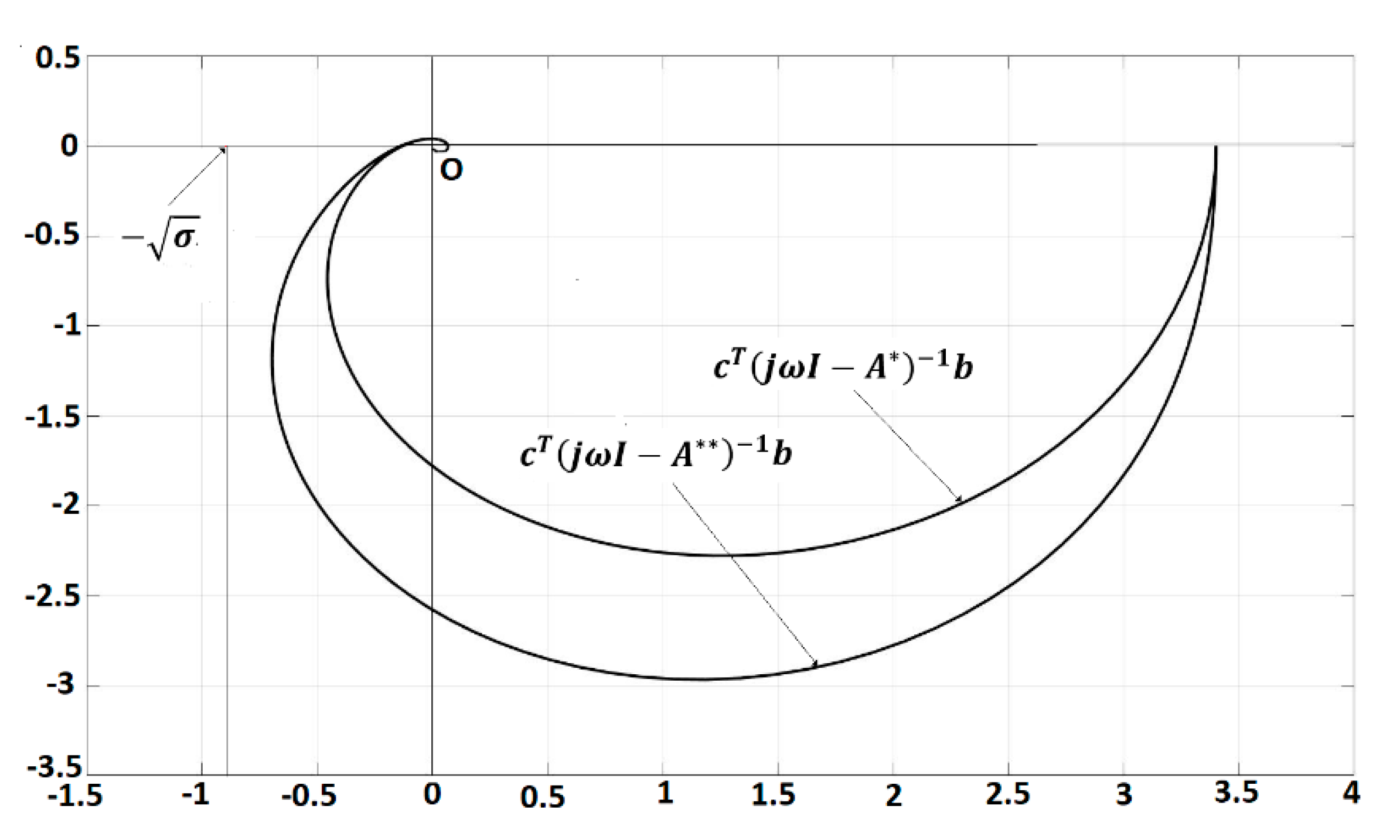
• Frequency criterion for linear FOS is proposed. Lyapunov techniques and the methods that derive from Yakubovici-Kalman-Popov Lemma [40] are used and the criteria that ensure asymptotic stability of the closed loop system are inferred. The criterion is extended to linear FOS with nonlinear components.
• Frequency criterion for time delay FOS is proposed using an approximate model based on Grunwald-Letnikov formula. The result is extended to the systems with nonlinear components.
• Stability criterion is proposed for systems composed of fractional order subsystems.
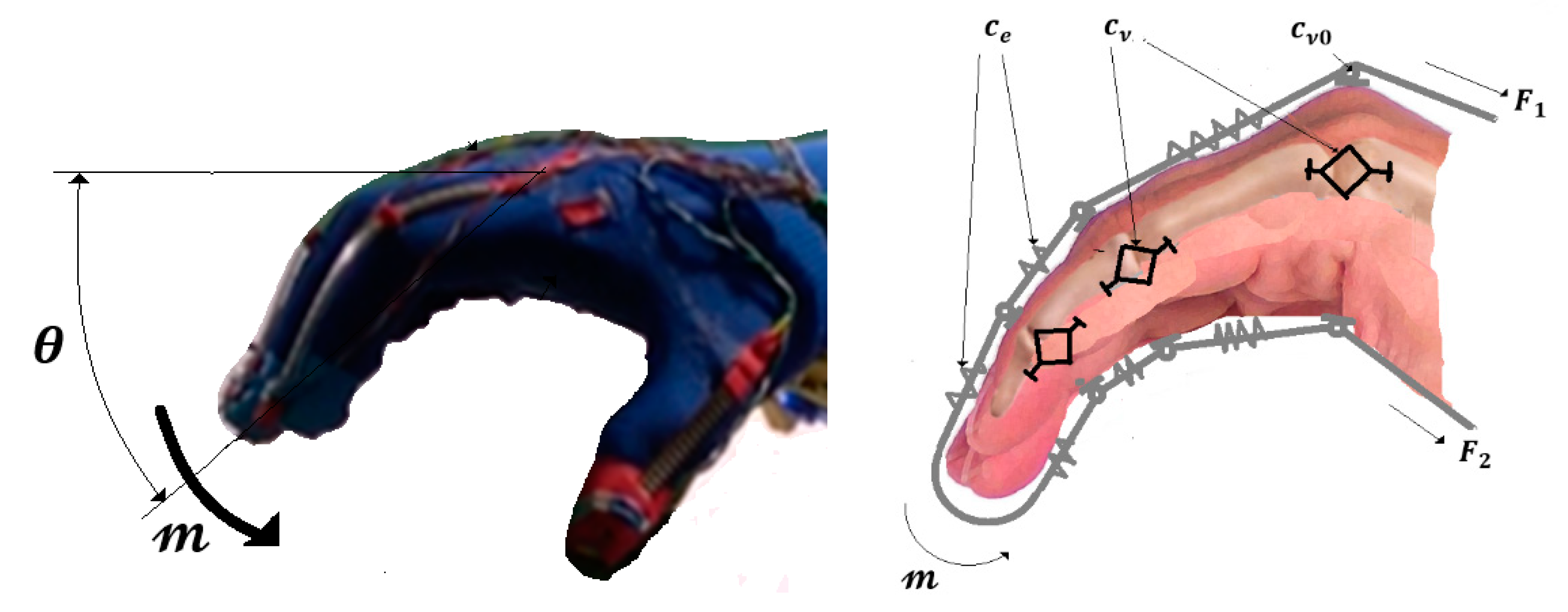
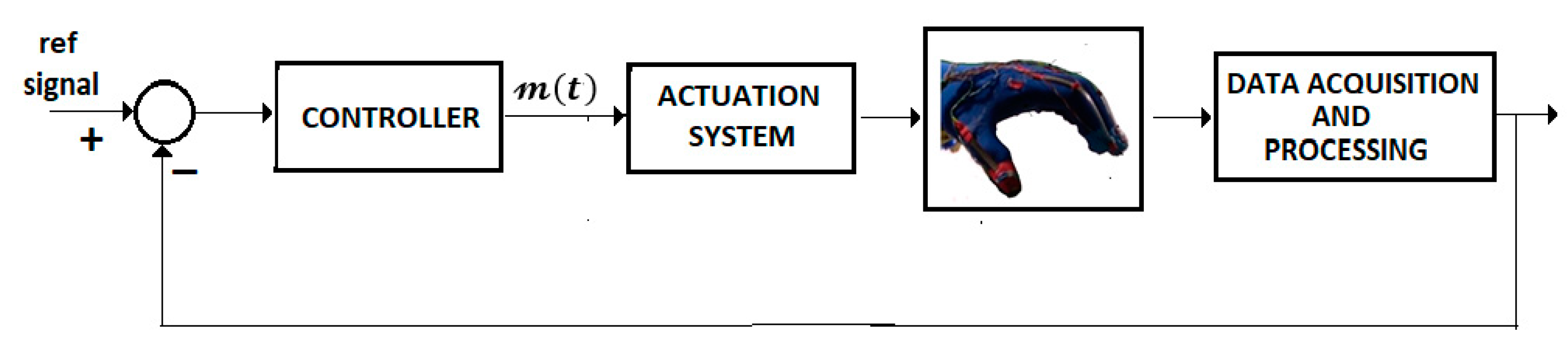
• The proposed methods have been implemented on two major applications: Soft Exoskeleton Glove Control that is studied as a nonlinear FOS model with time delay and Disabled Man-Wheelchair system that is studied as a fractional-order multi- system.

The paper is structured as follows: Section 2 presents mathematical preliminaries, and the control techniques proposed in this paper, Section 3 treats two applications: Soft Exoskeleton Glove Control and Disabled Man-Wheelchair system control, Section 4 is dedicated to Discussion and Section 5 presents Conclusions.

2. Control Techniques

Notations 1.

Let$X\in R^{n\times n}$be a real matrix. We denote the eigenvalues of$X$by${\lambda }_i\left(X\right).$We denote by${\lambda }_{min\left(X\right)}, {\lambda }_{max\left(X\right)}$, the minimum eigenvalue and maximum eigenvalue of$X,$respectively. Write$X\succcurlyeq (\succ )0,$if$X$is a positive semidefinite (positive definite) matrix.$X\succcurlyeq Y$if$X-Y\succcurlyeq 0$. The identity matrix in$R^{n\times n}$is shown by I. Let$z\in R^n$be a vector, $\Vert z\Vert ={\left({{\displaystyle \sum }}^{}{z}_i^2\right)}^{\frac{1}{2}}$. We denote by$j$the complex number, $j^2=-1$.

2.1. Mathematical Preliminaries

Lemma 1.

Ref. [29] For matrix $PϵR^{nxn}$, $P=P^T\succ 0,$the following inequality holds:

$${\lambda }_{\min \left(P\right)}\mathrm{I}\preccurlyeq P\preccurlyeq {\lambda }_{\max \left(P\right)} \mathrm{I}$$

Consider the fractional order system

$$D^{\beta }z\left(t\right)=Az\left(t\right)$$

(1)

where $D^{\beta }z\left(t\right)$ is the Caputo derivative of $z\left(t\right)$ for $0<\beta <1$.

Definition 1.

The matrix$A$is Hurwitz stable if

$$Arg\left(eig\left(A\right)\right)>\frac{\pi }{2}$$

(2)

Definition 2.

The matrix$A$is$\beta$-fractional order stable if

$$Arg\left(eig\left(A\right)\right)>\beta \frac{\pi }{2}$$

(3)

Theorem 1.

Refs. [6,14,15] The system (1), where $A$ is $\beta$-fractional order stable, is asymptotically stable.

Theorem 2.

Refs. [6,9,14,15] The system $D^{\beta }z\left(t\right)=f\left(z\left(t\right)\right), z\left(t_0\right)=z_0$ is asymptotically stable if there exist a continuously differentiable function $V\left(t,z\right)$ that satisfies

$${\alpha }_1{\Vert z\Vert }^2\le V\left(t,z\left(t\right)\right)\le {\alpha }_2{\Vert z\Vert }^2$$

(4)

$$D^{\beta }V\left(t,z\left(t\right)\right)\le -{\alpha }_3{\Vert z\Vert }^2$$

(5)

where ${\alpha }_1, {\alpha }_2, {\alpha }_3$ are positive constants, $0<\beta <1$.

Lemma 2.

Refs. [16,18] Let $z(.)\in R^n$ be a differentiable vector function. Then, the following inequality holds:

$$\frac{1}{2}{D}^{\beta }\left[z^T\left(t\right)z\left(t\right)\right]\le z^T\left(t\right)D^{\beta }z\left(t\right), \beta \in \left(0,1\right), t\ge t_0$$

(6)

2.2. Control Algorithms

2.2.1. Fractional Order Linear Systems (FOLS)

Consider the following FOLS model

$$D^{\beta }z\left(t\right)=Az\left(t\right)+bu\left(t\right)$$

(7)

$$z\left(t_0\right)=z_0$$

(8)

$$y\left(t\right)=c^{T}z\left(t\right)$$

(9)

where $D^{\beta }z\left(t\right)$ is the Caputo derivative of $z\left(t\right)$ for $0<\beta <1$, $A, b, c$ are $\left(n\times n\right), \left(n\times 1\right), \left(n\times 1\right)$ respectively, constant matrices, $z\in S \complement R^n, y\in R^1, u\in R^1$ are the system state, output and input.

Consider the following control law

$$u\left(t\right)=-ky\left(t\right)$$

(10)

where the controller gain $k=k_1+k_2$ is a positive constant that verifies the conditions

$$Arg(eig\left(\left(A-k_{1}b{c}^T\right)\right)>\frac{\pi }{2}$$

(11)

$$k_2\sigma \le 1$$

(12)

and $\sigma$ is a positive constant.

Theorem 3.

The system (7)–(12) which satisfies the following condition

$$Re\left(c^T{\left(j\omega \mathrm{I}-\left(A-k_{1}b{c}^T\right)\right)}^{-1}b\right)\ge -\sqrt{\sigma },,\forall \omega \in \left(-\infty ,+\infty \right)$$

(13)

is asymptotically stable.

Proof. 

The following Lyapunov function will be considered

$$V\left(z\right)=z^{T}Pz$$

(14)

where $P=P^T\succ 0$. This function verifies the conditions of Theorem 2 for ${\alpha }_1={\lambda }_{\min \left(P\right)},{\alpha }_2={\lambda }_{\max \left(P\right)}$ [7,15].

$$D^{\beta }V\left(z\right)\le \left(D^{\beta }{z}^T\right)Pz+z^{T}P\left(D^{\beta }z\right)$$

(15)

By evaluating (15) along the solutions of (7)–(10), yields

$$D^{\beta }V\left(z\right)\le z^T\left({\left(A-k_{1}b{c}^T\right)}^{T}P+P\left(A-k_{1}b{c}^T\right)\right)z+2{\mathit{z}}^{\mathit{T}}Pb{u}_2$$

(16)

where $u_2=-k_{2}y.$ This inequality can be rewritten as

$$D^{\beta }V\left(z\right)\le z^T\left({\left(A-k_{1}b{c}^T\right)}^{T}P+P\left(A-k_{1}b{c}^T\right)\right)z+2{\mathit{z}}^{\mathit{T}}Pb{u}_2-z^{T}c{u}_2+y{u}_2$$

(17)

Then by (10) and (12) it follows that

$$y{u}_2<-\sigma u_2^2$$

(18)

Substituting this result into (17) results in

$$D^{\beta }V\left(z\right)\le z^T\left({\left(A-k_{1}b{c}^T\right)}^{T}P+P\left(A-k_{1}b{c}^T\right)\right)z+2z^{\mathit{T}}\left(Pb-\frac{1}{2}c\right)u_2-\sigma u_2{}^2$$

(19)

By employing Yakubovici-Kalman-Popov (YKP) Lemma [40] and the condition (11), it follows that

$$z^T\left({\left(A-k_{1}b{c}^T\right)}^{T}P+P\left(A-k_{1}b{c}^T\right)\right)z=-q{q}^T$$

(20)

$$Pb-\frac{1}{2}c=\sqrt{\sigma }q$$

(21)

Now, substituting this result into (19) and considering the control law (10), it yields

$$D^{\beta }V\left(\mathit{z}\right)\le -z^T\left(q+k_2\sqrt{\sigma }c\right){\left(q+k_2\sqrt{\sigma }c\right)}^{T}z$$

(22)

or,

$$D^{\beta }V\left(\mathit{z}\right)\le -\rho {\Vert z\Vert }^2$$

(23)

where

$$\rho =\Vert \left(q+k_2\sqrt{\sigma }c\right){\left(q+k_2\sqrt{\sigma }c\right)}^T\Vert$$

(24)

□

2.2.2. Fractional Order Linear Systems with Nonlinear Components

Consider the following system

$$D^{\beta }z\left(t\right)=Az\left(t\right)+bu\left(t\right)+f\left(z\left(t\right)\right)$$

(25)

where $A, b, c$ are defined as in (7), (9) and $f\left(z\right)$ is a nonlinear function ($f:R^n\to R^n, f\left(0\right)=0)$ that satisfies the condition

$$\left|z^{T}f\left(z\right)\right|\le \mu {\Vert z\Vert }^2, \mu >0$$

(26)

Consider the control law (10)–(12).

Theorem 4.

The system (25), (9) with the control law (10)–(12), which satisfies the following condition

$$Re\left(c^T{\left(j\omega I-A^{*}\right)}^{-1}b\right)\ge -\sqrt{\sigma },,\forall \omega \in \left(-\infty ,+\infty \right)$$

(27)

is asymptotically stable, where

$$A^{*}=A-k_{1}b{c}^T+\mu \zeta \left(Q\right) \mathrm{I}$$

(28)

is a Hurwitz matrix and$P$is the solution of the Lyapunov equation,$A^{*}P+P{A}^{*}=-q{q}^T=-Q$and$\Vert P\Vert <{\lambda }_{max\left(P\right)}<\zeta \left(Q\right), \zeta$represents the upper matrix bound of$P$[29].

Proof. 

The proof is similar to that for Theorem 1. □

2.2.3. Time Delay Fractional Order Linear Systems (TDFOLS)

Consider the following TDFLOS model:

$$D^{\beta }z\left(t\right)=Az\left(t\right)+A_{1}z\left(t-\tau \right)+bu\left(t\right), \mathrm{t}\in \left[0,\mathrm{T}\right],\tau \in \mathbf{\Im }$$

(29)

z(t) = φ(t), t ∈ [−τ, 0]

(30)

$$y\left(t\right)=c^{T}z\left(t\right),$$

(31)

where $0<\beta <1$, $A,A_1,b,c$ are $\left(n\times n\right),\left(n\times n\right),\left(n\times 1\right),\left(n\times 1\right)$respectively, constant matrices, $z\in R^n,y\in R^1,u\in R^1$ are the system state, output, and input.

Consider the control law

$$u\left(t\right)=-ky\left(t\right)$$

(32)

Assumption 1.

The following constraint is satisfied:

$$\left|z^T\left(t-\tau \right)z\left(t\right)\right|\le \alpha \left(\tau \right)z^T\left(t\right)z\left(t\right), \tau \in \mathbf{\Im }$$

(33)

where$\mathbf{\Im }=[{\tau }_{min}, {\tau }_{max}]$and $\alpha \left(\tau \right)$can be approximated by a linear relation

$$\alpha \left(\tau \right)={\alpha }_1+{\alpha }_2{\tau }^{\beta }, \tau \in \mathbf{\Im }$$

(34)

or,

$$\left|z^T\left(t-\tau \right)\Vert z\left(t\right)\Vert \right|\le {\alpha }_{max}z\left(t\right)$$

(35)

Assumption 2.

There exist the control gain$k_1>0,$$(k_1<k)$such that

$$A^{*}=A-k_1 b{c}^T, \tau \in \mathbf{\Im }$$

(36)

is a Hurwitz matrix. As in the previous sections, consider that$k_2=k-k_1$verifies the condition

$$k_2\sigma \le 1$$

(37)

Theorem 5.

The system (29)–(31), with the control law (32) and which satisfies the following condition

$$Re\left(c^T{\left(j\omega I-A^{*})\right)}^{-1}b\right)\ge -\sqrt{\sigma } ,\forall \omega \in \left(-\infty ,+\infty \right)$$

(38)

$$\rho -{\rho }^{*}>0$$

(39)

is asymptotically stable, where$\rho ,{\rho }^{*}$are defined by (26), (42), respectively.

Proof. 

The Lyapunov function (16) is considered and, using the same techniques as in Section 2.2.1, taking into account the control law (32), the conditions (36), (37), and YKP Lemma (22), (23), it is obtained

$$D^{\beta }V\left(z\left(t\right)\right)\le -z{\left(t\right)}^T\left(q+k_2\sqrt{\sigma }c\right){\left(q+k_2\sqrt{\sigma }c\right)}^{T}z\left(t\right)+z{\left(t\right)}^T\left(A_1^{T}P+P{A}_1\right)z\left(t-\tau \right)$$

(40)

Therefore, applying inequalities (33), (35) yields

$$D^{\beta }V\left(z\left(t\right)\right)\le -z{\left(t\right)}^T\left(q+k_2\sqrt{\sigma }c\right){\left(q+k_2\sqrt{\sigma }c\right)}^{T}z\left(t\right)+{\rho }^{*}\Vert z{\left(t\right)\Vert }^2$$

(41)

where

$${\rho }^{*}={\lambda }_{\max \left(A_1^{T}P+P{A}_1\right)}{\alpha }_{max}$$

(42)

The inequality (41) can be rewritten as

$$D^{\beta }V\left(z\left(t\right)\right)\le -\left( \rho -{\rho }^{*}\right)\Vert z{\left(t\right)\Vert }^2$$

(43)

where $\rho$ is given by (26). □

Remark 1.

The result of Theorem 3 can be easily extended to systems with nonlinear components,

$$D^{\beta }z\left(t\right)=Az\left(t\right)+A_{1}z\left(t-\tau \right)+f\left(z\right)+bu\left(t\right), \mathrm{t}\in \left[0,\mathrm{T}\right],\tau \in \mathbf{\Im }$$

(44)

where$f\left(z\right)$verifies the condition (26). In this case, the frequential condition (38) is verified for$A^{*}+\mu \zeta \left(Q\right) I$, where$\mu , \zeta , Q$are defined in Section 2.2.2.

2.2.4. Systems Composed of Linear Fractional Order Subsystems

Consider the linear systems

$$D^{\beta }{z}^i\left(t\right)=A_i{z}^i\left(t\right), i=1,2,\dots ,N$$

(45)

$$z^i\left(t_0\right)=z_0^i$$

(46)

where the exponent, $A_i$is a $\left(n_i\times n_i\right)$constant matrix, $z^i\in S^i \complement R^{n_i}$ In the composite system, a number of components can be $\beta$-fractional order stable systems,

$$Arg\left(eig\left(A_j\right)\right)>\beta \frac{\pi }{2}, j=1,2,\dots ,K, K\le N$$

(47)

Consider the Lyapunov function associated with each system $i, \left(V_i:R^{n_i}\to R^1\right),$

$$V_i\left(z^i\left(t\right)\right)=z^{i }{}^T\left(t\right)z^{i }\left(t\right)$$

(48)

From (4) and Lemma 1 (6), yields

$$D^{\beta }{V}_i\left(z^i\left(t\right)\right)\le 2z^{i }{}^T\left(t\right)D^{\beta }\left(z^{i }\left(t\right)\right)=2z^{i }{}^T\left(t\right)A_i{z}^i\left(t\right), i=1,2,\dots ,N$$

(49)

or

$$D^{\beta }{V}_i\left(z^i\left(t\right)\right)\le 2{\lambda }_{\max \left(A_i\right)}{z}^{i }{}^T\left(t\right)z^{i }\left(t\right)=2{\lambda }_{\max \left(A_i\right)}{V}_i\left(z^i\left(t\right)\right)$$

(50)

Consider the following composite system

$$D^{\beta }{z}^i\left(t\right)=A_i{z}^i\left(t\right)+{{\displaystyle \sum }}_{j=1}^N{B}_{ij}{z}^j\left(t\right), i=1,2,\dots ,N$$

(51)

where $B_{ij}$ is a $\left(n_i\times n_j\right)$inter-connection matrix that satisfies the following condition

$$z^{i }{}^T\left(t\right){\displaystyle \sum }_{j=1}^N{B}_{ij}{z}^j\left(t\right)\le {{\displaystyle \sum }}_{j=1}^N{\gamma }_{ij}{z}^{j }{}^T\left(t\right) z^{j }\left(t\right), i=1,2,\dots ,N$$

(52)

where the following inequalities were used [29]:

$$z^{i }{}^T\left(t\right)B_{ij}{z}^j\left(t\right)\le \Vert B_{ij}\Vert \Vert z^{i }\left(t\right)z^j\Vert \Vert \left(t\right)\Vert$$

(53)

$$\Vert z^{i }\left(t\right)\Vert \Vert z^j\left(t\right)\Vert \le z^{i }{}^T\left(t\right)z^{i }\left(t\right)+z^{j }{}^T\left(t\right)z^{j }\left(t\right)$$

(54)

Consider that the composite system state vector is

$$z={\left[\begin{array}{ccc}{z}^{1 }& z^{2 }& \begin{array}{cc}\dots & z^{N }\end{array}\end{array}\right]}^T\in S=\left(S_1\times S_2\times \dots \times S_N\right)$$

(55)

Theorem 6.

The composite system (45), (51) which satisfies the following condition

$$Arg\left(eig(ℳ)\right)>\beta \frac{\pi }{2}$$

(56)

is asymptotically stable,

where

$$ℳ=\left[\begin{array}{ccc}{\lambda }_{\max \left(A_1\right)}+{\displaystyle \sum }_1^N{\gamma }_{1j}& {\gamma }_{12}& \begin{array}{cc}\dots & {\gamma }_{1N}\end{array}\\ {\gamma }_{21}& {\lambda }_{\max \left(A_2\right)}+{\displaystyle \sum }_1^N{\gamma }_{2j}& \begin{array}{cc}\dots & {\gamma }_{2N}\end{array}\\ \begin{array}{c}\dots \\ {\gamma }_{N1}\end{array}& \begin{array}{c}\dots \\ {\gamma }_{N2}\end{array}& \begin{array}{cc}\begin{array}{c}\dots \\ \dots \end{array}& \begin{array}{c}\dots \\ {\lambda }_{\max \left(A_N\right)}+{\displaystyle \sum }_1^N{\gamma }_{Nj}\end{array}\end{array}\end{array}\right].$$

(57)

Proof. 

Consider the following vector Lyapunov function, $\left(V:R^{{{\displaystyle \sum }}^{}{n}_i}\to R^N\right)$

$$\left(z\right)={\left[\begin{array}{ccc}{V}_1\left(z^{1 }\right)& V_2\left(z^{2 }\right)& \begin{array}{cc}\dots & V_N\left(z^{N }\right)\end{array}\end{array}\right]}^T$$

(58)

where $V_i, i=1,2,\dots ,N$ are defined by (48), $V(z$) is a continuously differentiable vector function and

$$V\left(z\left(t_0\right)\right)=V_0$$

(59)

where

$$\Vert V_0\Vert <\delta$$

(60)

and $\delta$ is a positive constant.

The fractional derivation of (14) is

$$D^{\beta }V\left(z\right)={\left[\begin{array}{ccc}{D}^{\beta }{V}_1\left(z^{1 }\right)& D^{\beta }{V}_2\left(z^{2 }\right)& \begin{array}{cc}\dots & D^{\beta }{V}_N\end{array}\end{array}\left(z^{N }\right)\right]}^T$$

(61)

and according with (48), (50), and Lemma 1 (6), yields

$$D^{\beta }{V}_i\left(z^{i }\left(t\right)\right)\le 2z^{i }{}^T\left(t\right)D^{\beta }\left(z^{i }\left(t\right)\right)=2z^{i }{}^T\left(t\right)(A_i{z}^i\left(t\right)+{{\displaystyle \sum }}_{j=1}^N{B}_{ij}{z}^j\left(t\right).$$

(62)

By employing inequality (52) one derives that

$$D^{\beta }{V}_i\left(z^{i }\right)\le 2\left({\lambda }_{\max \left(A_i\right)}+{{\displaystyle \sum }}_{i=1}^N{\gamma }_{ij}\right)z^{i }{}^T\left(t\right)z^{i }\left(t\right)+{{\displaystyle \sum }}_{\begin{array}{c}j=1\\ j\ne i\end{array}}^N{\gamma }_{ij}{z}^{j }{}^T\left(t\right) z^{j }\left(t\right))$$

(63)

or,

$$D^{\beta }{V}_i\left(z^{i }\right)\le 2\left({\lambda }_{\max \left(A_i\right)}+{{\displaystyle \sum }}_{i=1}^N{\gamma }_{ij}\right)V_i\left(z^{i }\right)+{{\displaystyle \sum }}_{\begin{array}{c}j=1\\ j\ne i\end{array}}^N{\gamma }_{ij}{V}_j\left(z^{j }\right)$$

(64)

From (59), it follows that

$$D^{\beta }V\left(z\left(t\right)\right)=2ℳV\left(z\left(t\right)\right)$$

(65)

If the condition (56) is satisfied, the system (65) is asymptotically stable, such that

$$\underset{t\to \infty }{\lim }\Vert V(z\left(t\right)\Vert =0$$

(66)

It can be concluded that

$$\underset{t\to \infty }{\lim }{V}_i\left(z^{i }\left(t\right)\right)=0, i=1,2,\dots ,N$$

(67)

or,

$$\underset{t\to \infty }{\lim }(z^{i }\left(t\right))=0, i=1,2,\dots ,N\mathrm{QED}$$

(68)

The control strategy proposed by Theorem 4 based on the Lyapunov vector function (58) allows the use of $\left(N\times N\right)$ matrix operators instead of (${{\displaystyle \sum }}^{}{n}_i\times {{\displaystyle \sum }}^{}{n}_i)$ operators as used in [38,39], which considerably simplifies the calculation and implementation effort. □

2.2.5. Control Systems-Conclusions

The previous sections discussed the control laws for several classes of models described by fractional-order equations: Fractional Order Linear Systems, Fractional Order Linear Systems with nonlinear components, Time Delay Fractional Order Linear Systems, Time Delay Fractional Order Linear Systems with nonlinear components. The control law was determined for these systems as, $u\left(t\right)=-ky\left(t\right)$ where the controller gain $k=k_1+k_2$ and $k_2$ verifies the condition $k_2\sigma \le 1$. The component $k_1$ satisfies the frequency condition: $Re\left(G(j\omega \right))\ge -\sqrt{\sigma },\forall \omega \in \left(-\infty ,+\infty \right)$, where $G(j\omega$) is determined by (13), (28), (36), for each class of systems. This inequality can be interpreted as the Nyquist criterion for the critical point $-\sqrt{\sigma }.$

3. Results

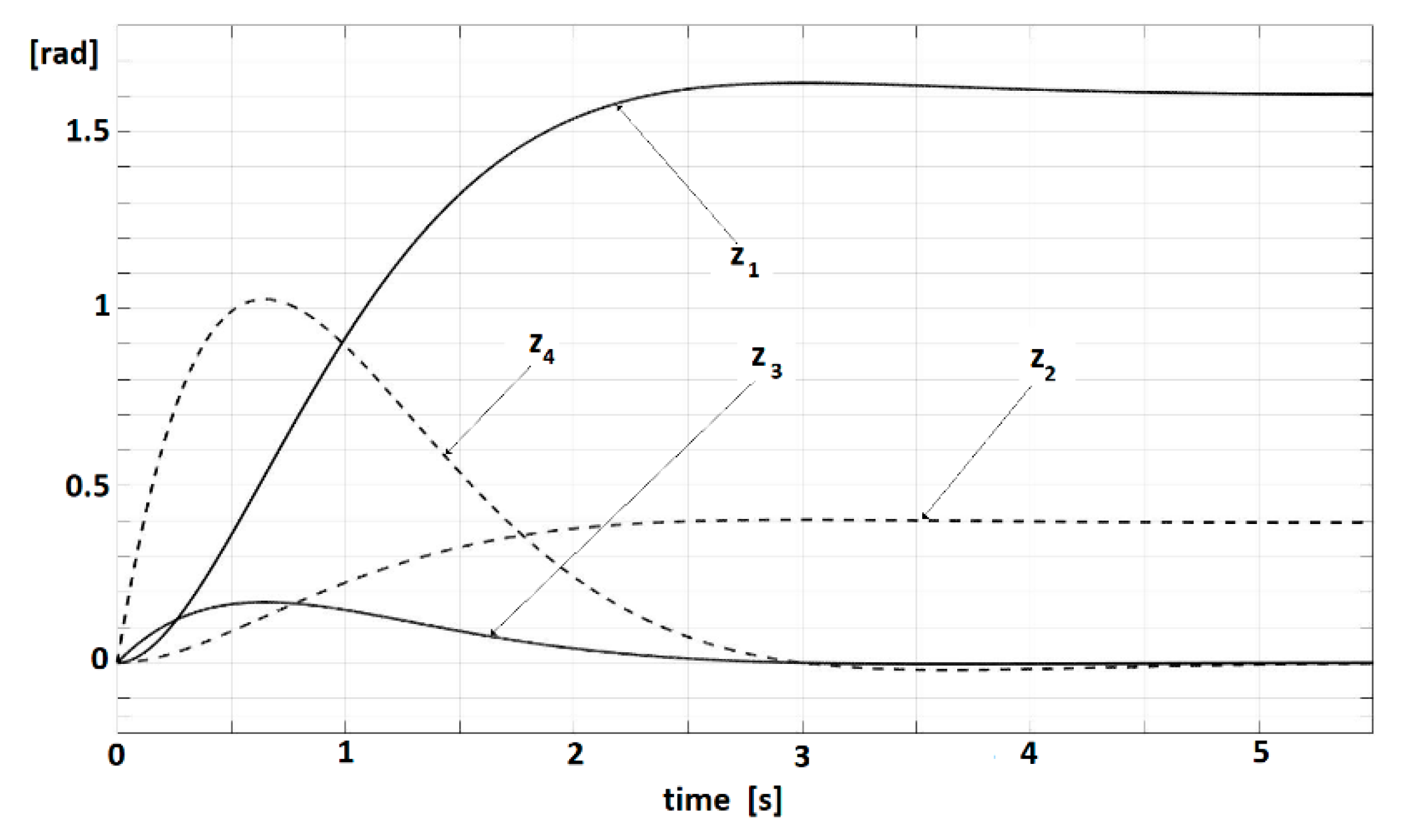
3.1. Soft Exoskeleton Glove Control

An illustrative example of FOLS models is the model of a biomechanical system of a glove exoskeleton used to restore human functions for people with disabilities or who have suffered various traumas. Figure 1 shows the architecture of such a system that represents a complex structure of muscle tissues combined with elements of mechanical structure. An advanced conceptual analysis of the dynamics of these systems indicates the use of fractional calculus in Maxwell’s classic stress-strain models [41,42].

3.1.1. Case 1-FOLS Model

The dynamic model of this system can be described by the second order transfer function with fractional order component β = 1.5,

$$Y\left(s\right)=\frac{\theta \left(s\right)}{𝓂\left(s\right)}=\frac{k_h}{J{s}^2+c_{\nu }{s}^{\beta }+c_{\nu 0}s+c_e}$$

(69)

where $\theta$ is the equivalent angular position of the hand, $𝓂$ is the moment exercised by the driving forces, $J$ is the equivalent inertia moment and $c_{\nu }, c_{\nu 0}, c_e$ denote coefficients of viscosity and elasticity, respectively, and $k_h$ is the gain coefficient. The time model can be written as

$$J \ddot{\theta }\left(t\right)+c_{\nu }{D}^{\beta }\theta \left(t\right)+c_e \theta \left(t\right)+c_{\nu 0} \dot{\theta }\left(t\right)=k_h𝓂\left(t\right)$$

(70)

where the Maxwell’s term has the fractional exponent with $\beta$ =1.5. The state vector $z={\left[z_1, z_2,z_3,z_4\right]}^T$ is defined as

$$z_1=\theta ; D^{0.5}{z}_1=z_2; D^{0.5}{z}_2=D^1{z}_1=z_3,D^{0.5}{z}_3=D^1{z}_1=z_4={\theta }^{1.5},D^{0.5}{z}_4=\ddot{\theta }$$

The state model can be obtained as

$$D^{0.5}z\left(t\right)=Az\left(t\right)+b u\left(t\right)$$

(71)

A more complete form also includes a nonlinear term determined by the gravitational components

$$D^{0.5}z\left(t\right)=Az\left(t\right)+g\left(z\right)+b u\left(t\right)$$

(72)

$$z\left(0\right)=z_0=0$$

(73)

where $𝓂$ is the control vector and $A, b, g$are $\left(4\times 4\right)$, $\left(4\times 1\right), \left(4\times 1\right)$matrices, respectively,

$$A=\left[\begin{array}{cc}\begin{array}{cc}0& 1\end{array}& \begin{array}{cc}0& 0\end{array}\\ \begin{array}{cc}0& 0\end{array}& \begin{array}{cc}1& 0\end{array}\\ \begin{array}{cc}\begin{array}{c}0\\ -c_e/J \end{array}& \begin{array}{c}0\\ 0\end{array}\end{array}& \begin{array}{cc}\begin{array}{c}0\\ -c_{\nu 0}/J\end{array}& \begin{array}{c}1\\ -c_{\nu }/J\end{array}\end{array}\end{array}\right];b=\left[\begin{array}{c}0\\ \begin{array}{c}0\\ 0\\ k_h/J\end{array}\end{array}\right];c=\left[\begin{array}{c}{c}_1\\ \begin{array}{c}{c}_2\\ c_3\\ c_4\end{array}\end{array}\right]$$

(74)

The output of the system $y\left(t\right)$ is evaluated by direct measuring of the angular position $z_1=\theta$ and by estimation of fractional variables $z_2, z_3$ by using the Gr$\ddot{u}$nwald-Letnikov’s formula,

$$y\left(t\right)=c^T z\left(t\right)$$

(75)

The nonlinear component $g\left(z\right)$ verifies the inequality (26) with $\mu =2\times {10}^{-3}$. The dynamic system is described by the following parameters [34]: the equivalent inertia is $J=14\times {10}^{-5}\mathrm{kg}.{\mathrm{m}}^2$, the viscous and elastic coefficients of the joint tissues throughout phalange musculoskeletal system and glove are $c_{\nu }=0.408\times {10}^{-2}\mathrm{Nm}.\mathrm{s}.{\mathrm{rad}}^{-1}$, $c_e=0.27\times {10}^{-2}\mathrm{Nm}.{\mathrm{rad}}^{-1}$, respectively and the damping coefficient is $c_{\nu 0}=0.324\times {10}^{-2}\mathrm{Nm}.\mathrm{s}.{\mathrm{rad}}^{-1}$.

The matrix $A$ is $1/2-fractionalstable,$($Arg\left(eig\left(A\right)\right)>\frac{\pi }{4}$, with (${\lambda }_1=-33.48,{\lambda }_2=-1.29,{\lambda }_3=0.185+j0.65,{\lambda }_4=0.185-j0.65).$ According with Theorem 2, a controller (Figure 2) with $k_1=2.4$ is proposed. A matrix $Q=q{q}^T=diag\left(0.10.10.10.1\right]$ is used for Lyapunov Equation (22). The upper matrix bound ${\lambda }_{\max \left(P\right)}=\zeta \left(Q\right)=96.8$is evaluated [29]. The matrix $A^{*}=A-k_{1}b{c}^T+\mu \zeta \left(Q\right)\mathrm{I}$ is a Hurwitz matrix (${\lambda }_1=-31.25,{\lambda }_2=-2.75,{\lambda }_3=-0.199+j1.005,{\lambda }_4=-0.199-j1.005).$ The second component is selected as $k_2=1.5,\sigma =0.64$ that satisfies the inequality (12). The frequency condition (13) is verified in Figure 3.

MATLAB/SIMULINK methods are used for the simulation [4,10]. The variable trajectories, the physical significance variables as angular position, and the estimated variables by Mittag-Leffler techniques, $z_2, z_3, z_4$ are shown in Figure 4. The asymptotic stability of all variables, measurable physical significance, and estimated virtual variables is well highlighted. Note the evolution of the angular variable $\theta$, the variable that defines the main coordinate of movement, that satisfies the parameters: the settling time $T_s$ and the peak time $T_p$ verifies the condition $\raisebox{1ex}{$T_p$}\!\left/ \!\raisebox{-1ex}{$T_s$}\right.<0.5$ for $T_s=5\mathrm{s}$ with an overshoot $\delta <0.05\%$ [40].

3.1.2. Case 2-TDFOLS Model

The reaction time of the man with disabilities, determined by the propagation time in the nervous system as well as the time constants of the muscular system, introduces a delay component $\tau$. Through this component, the dynamic model (69) becomes

$$Y_D\left(\mathrm{s}\right)=Y\left(s\right)e^{-\tau s}$$

(76)

It is very difficult to evaluate this time delay. Experimental results [42] allow us to identify a domain $\mathbf{\Im }=\left[0.1;0.5\right]s$,$\tau \in \mathbf{\Im }.$ In time domain, the transfer function, becomes

$$D^{\beta }z\left(t\right)=Az\left(t\right)+A_{1}z\left(t-\tau \right)+bu\left(t\right), \mathrm{t}\in \left[0,\mathrm{T}\right],\tau \in \mathbf{\Im }$$

(77)

z(t) = 0, t ∈ [−τ, 0]

(78)

$$y\left(t\right)=c^{T}z\left(t\right),$$

(79)

where $A_{1}z\left(t-\tau \right)$ is determined by the human decision

$$m\left(t-\tau \right)=k_h{b}_h{c}_h^{T}z\left(t-\tau \right)$$

(80)

and the matrix coefficients are defined as in (74). According with Theorem 3, a controller with $k_1^{*}=7.4$ is used. The matrix $A^{**}=A-k_1^{*} b{c}^T+\mu \zeta \left(Q\right) \mathrm{I}$ is Hurwitz stable (${\lambda }_1=-23.69, {\lambda }_2=-1.4,{\lambda }_3=-0.35,{\lambda }_4=-0.56)$. The gain $k_2$ is selected as $k_2=3.5$to satisfy the constraint (37) for $\sigma =0.25$. The factor $\rho$ is evaluated, $\rho$ =3.2, and the parameter ${\rho }^{*}$ is estimated as ${\rho }^{*}=1.6$for $\tau \in \left[0.1, 0.5\right]\mathrm{s}$. The frequency condition (38) is verified (Figure 3) and the condition (39) is satisfied. The system trajectories are shown in Figure 5. As in the previous example, we remark the asymptotic stability of all variables, measurable physical significance, and estimated virtual variables. Regarding the angular variable $\theta$, the transient response satisfies the parameters: $\raisebox{1ex}{$T_p$}\!\left/ \!\raisebox{-1ex}{$T_s$}\right.<0.5$ for $T_s=6\mathrm{s}$ with an overshoot $\delta <0.08\%.$

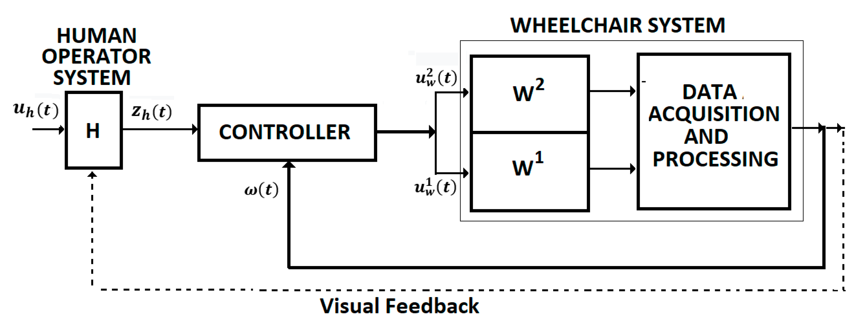
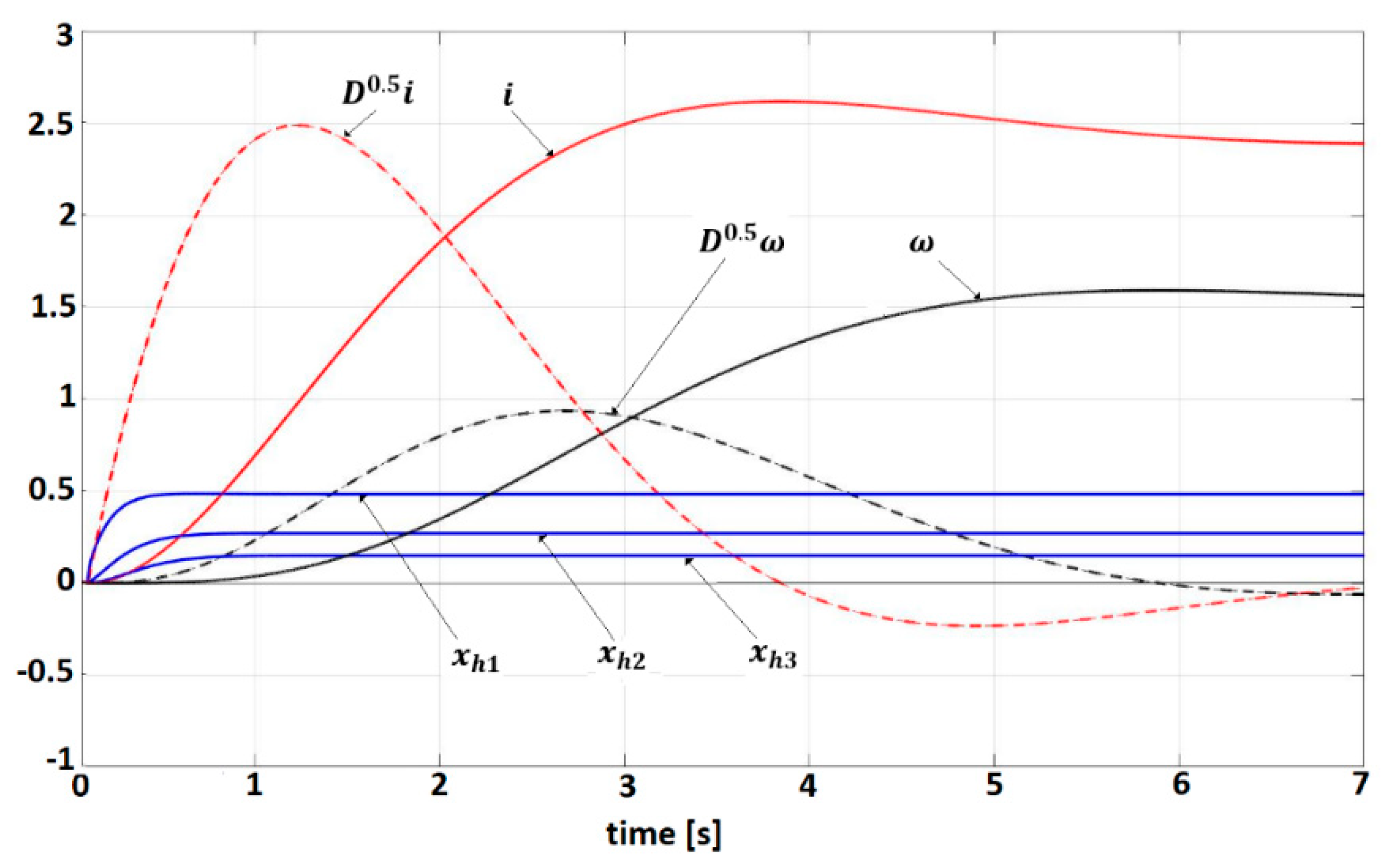
3.2. Disabled Man-Wheelchair System Control

One of the most interesting control applications of some systems defined by fractional order models is the one referring to the control exercised by a disabled person, with health problems regarding locomotor disabilities or cerebral deficiency. Such an example may occur in a person with Parkinson’s who drives a wheelchair (Figure 6). This system can be considered as a composite system with two sub-systems: the human operator and the wheelchair.

The existence of a handicap of the human operator determines a wheelchair driving with very low performances. For this reason, it is necessary to introduce a controller to improve the control of the movement on the imposed trajectories, (Figure 7). The dynamics of human operator are better characterized by fractional models that more correctly express the control strategy based on memorizing some observations from the history of evolution. The fractional order model is [43,44,45],

$$Y_h\left(\mathrm{s}\right)=\frac{x_h\left(s\right)}{u_h\left(s\right)}=\frac{k_h}{\left({\tau }_{h1}{s}^{0.5}+1\right)\left({\tau }_{h2}s+1\right)}$$

(81)

where $x_h$ is the human state, ${\tau }_{h1}, {\tau }_{h2}$ are human time constants, $k_h$ is the human gain (see Appendix A), $u_h$ defines the human control toward the target, the desired evolution expressed by a desired wheelchair orientation.

Rewritten (81) in time, yields

$$\begin{gathered} D^{0.5}{x}_{h1}\left(t\right)=x_{h2}\left(t\right) \\ \hspace{1em}\hspace{1em}\hspace{1em}\hspace{1em}\hspace{1em}\hspace{1em}\hspace{1em}\hspace{1em}\hspace{1em}\hspace{1em}\hspace{1em}\hspace{1em}\hspace{1em}\hspace{1em}\hspace{1em}\hspace{1em}{D}^{0.5}{x}_{h2}\left(t\right)=x_{h3}\left(t\right) \\ {D}^{0.5}{x}_{h3}\left(t\right)=-\frac{1}{{\tau }_{h1}}{x}_{h3}\left(t\right)-\frac{1}{{\tau }_{h2}}{x}_{h2}\left(t\right)-\frac{1}{{\tau }_{h1}{\tau }_{h2}}{x}_{h1}\left(t\right)+\frac{k_h}{{\tau }_{h1}{\tau }_{h2}}{u}_h\left(t\right) \end{gathered}$$

(82)

or

$$D^{0.5}{z}_h\left(t\right)=A_h{z}_h\left(t\right)+b_h{u}_h\left(t\right)$$

(83)

$$y_h\left(t\right)=c_h^T{z}_h\left(t\right)$$

(84)

where $z_h={\left[x_{h1},x_{h2},x_{h3}\right]}^T,c_h={\left[0,0,1\right]}^T$. The human system is ½-fractional order stable with ${\lambda }_{h1}=-0.0207,{\lambda }_{h2}=-0.0397+0.2163i$, ${\lambda }_{h3}=-0.0397-0.2163i$. The human behavior is defined by the derivative component [45],

$$x_{h3}\left(t\right)={\dot{x}}_h\left(t\right)={\sigma }_h^T{z}_w\left(t\right)$$

(85)

where ${\sigma }^h,\mathrm{a}(4\times 1)$ matrix, designates the influence of the components of $z_w$ on human behavior. The human control $u_h$ acts through a negative feedback determined by the information received from the driven system (the wheelchair),

$$u_h\left(t\right)=-k_h^{*}{c}_{hw}^T{z}_w\left(t\right)$$

(86)

where $c_{hw}$ is (4$\times 1)$ interconnection matrix between the two systems (Appendix A).

The model of the wheelchair is a classical wheelchair model [46] with the control of direction done by the control of the main wheel velocities and detremined by the joystick, The model represents a decoupled drive system, with symmetrical, electrical, and mechanical structure. This symmetry allows to use the following mathematical model

$${\dot{x}}_w^j\left(t\right)=A_v{x}_w^j\left(t\right)+b_w{u}_w^j\left(t\right), j=1,2$$

(87)

$$A_w=\left[\begin{array}{cc}-\nu /J& k_t/nJ\\ -k_e/L& -R/L\end{array}\right],b_w=\left[\begin{array}{c}0\\ 1/L\end{array}\right], j=1,2$$

(88)

where $x_w^j={\left[ {\omega }_j i_j\right]}^T$ defines the wheelchair state, $u_w^j$ is the input variable and (index $j=1, 2$ defines the motion direction, toward the left and right) and $R,L, J, k_t, k_e, n, \nu$ are the electrical and mechanical parameters of the system. The electrical and mechanical parameters are presented in Appendix A.

The fractional order state vector is defined as

$$z_w^j={\left[x_{w1}^j x_{w2}^j x_{w3}^j x_{w4}^j\right]}^T, j=1,2$$

(89)

where

$$\begin{gathered} x_{w1}^j={\omega }_j; D^{0.5}{x}_{w1}^j=x_{w2}^j;D^{0.5}{x}_{w2}^j=k_t/nJ{x}_{w3}^j-\nu /J x_{w1}^j \\ {x}_{w3}^j=i_j; D^{0.5}{x}_{w3}^j=x_{w4}^j;D^{0.5}{x}_{w4}^j=-R/L{x}_{w3}^j-k_e/L{x}_{w1}^j+1/L u_w^j; \end{gathered}$$

(90)

The dynamic model is

$$D^{0.5}{z}_w\left(t\right)=A_w{z}_w\left(t\right)+b_w{u}_w\left(t\right)$$

(91)

$$y_w\left(t\right)=c_w^T{z}_w\left(t\right)$$

(92)

where

$$A_w=\left[\begin{array}{ccc}\begin{array}{c}0\\ \raisebox{1ex}{$-\nu $}\!\left/ \!\raisebox{-1ex}{$J$}\right.\\ \begin{array}{c}0\\ \raisebox{1ex}{$-k_e$}\!\left/ \!\raisebox{-1ex}{$L$}\right.\end{array}\end{array}& \begin{array}{c}1\\ 0\\ \begin{array}{c}0\\ 0\end{array}\end{array}& \begin{array}{cc}\begin{array}{c}0\\ k_t/nJ\\ \begin{array}{c}0\\ -R/L\end{array}\end{array}& \begin{array}{c}0\\ 0\\ \begin{array}{c}1\\ 0\end{array}\end{array}\end{array}\end{array}\right];b_w=\left[\begin{array}{c}{0}_{3\times 1}\\ \raisebox{1ex}{$1$}\!\left/ \!\raisebox{-1ex}{$L$}\right.\end{array}\right]; c_w=\left[\begin{array}{c}{c}_{\omega }\\ 0_{3\times 1}\end{array}\right];$$

(93)

$$y_w\left(t\right)=c_w^T{z}_w\left(t\right)$$

(94)

The system (90)–(93) is Hurwitz stable (${\lambda }_{w1}=-4.3183+2.0636i,{\lambda }_{w2}=-4.3183-2.0636i,{\lambda }_{w3}=-3.3975+2.9886i,{\lambda }_{w4}=-3.3975-2.9886i$).

The controller implements the control law for the composite system

$$u_w\left(t\right)=-k_{wh}{d}_{wh}^T{z}_h\left(t\right)-k_{ww}{y}_w\left(t\right)$$

(95)

where $d_{wh}, \mathrm{a}\left(3\times 1\right)\mathrm{matrix},\mathrm{designates}$the human control components in the global control law (Appendix A).

As proposed in Section 2.2.4, we define the Lyapunov function of the composite system

$$V={\left[V_h V_w\right]}^T$$

(96)

where

$$V_h=z_h^T{z}_h$$

(97)

$$V_w=z_w^T{z}_w$$

(98)

$$D^{0.5}V={\left[D^{0.5}{V}_h D^{0.5}{V}_w\right]}^T$$

(99)

Using a similar technique as developed in the previous sections, from (83)–(86) and (91)–(94), yields,

$$D^{0.5}{V}_h\le {\lambda }_{\max \left(A_h\right)}{z}_h^T{z}_h-k_h^{*}{\lambda }_{\min \left(Q_{hw}\right)}{z}_w^T{z}_w$$

(100)

$$D^{0.5}{V}_w\le {\lambda }_{\max \left(A_w^{*}\right)}{z}_w^T{z}_w+k_{wh}{\lambda }_{\max \left(b{d}_{wh}^T\right)}{z}_h^T{z}_h$$

(101)

where $Q_{hw}={\sigma }_h{c}_{hw}^T$, $A_w^{*}=A_w-k_w{b}_w{c}_w^T+k_{wh}{\lambda }_{\max \left(b{d}_{wh}^T\right)}\mathrm{I}$. From (65), (99), obtain

$$D^{0.5}V=\left[\begin{array}{cc}\begin{array}{c}{\lambda }_{\max \left(A_h\right)}\\ k_{wh}{\lambda }_{\max \left(b{d}_{wh}^T\right)}\end{array}& \begin{array}{c}-k_h^{*}{\lambda }_{\min \left(Q_{hw}\right)}\\ {\lambda }_{\max \left(A_w^{*}\right)}\end{array}\end{array}\right] V$$

(102)

$$D^{0.5}V=2ℳV$$

(103)

The composite system is ½-fractional order stable: ${\lambda }_{ℳ1}=0.23+i0.45$, ${\lambda }_{ℳ2}=0.23-i0.45$with

$$Arg\left(eig(ℳ)\right)>\frac{\pi }{4}$$

(104)

The system trajectories, human operator, and wheelchair, for a desired target defined by ${\omega }_d$= π/2 rad are shown in Figure 8. The good quality of motion can be easily remarked. We remark the asymptotic stability of all variables, measurable physical significance, ${\omega }_i$ and estimated virtual variables, $D^{0.5}\omega$, $D^{0.5}i$ The same behavior is noticed in the parameters that define the human operator, $x_{h1}$,$x_{h2},x_{h3}$. Regarding the control angular variable ω, the transient response has an overshoot δ < 0.01%.

4. Discussion

The control techniques presented by the literature are based on algebraic criteria, matrix inequalities and frequency criteria. A selection of these criteria are presented in

Table 1. Control Techniques.

Papers	Systems	Control Techniques
1, 2, 4, 8, 13, 20, 21	Linear FOS	Algebraic criteria
3, 5, 6, 9, 12, 16, 17, 18, 19, 21	Nonlinear FOS	Algebraic criteria Matrix Inequalities
32, 33, 34	Linear FOS	Frequency criteria
11, 22, 24, 25, 26, 27, 28, 30	Delay FOS	Algebraic criteria

. Our paper presents a unitary control method for several classes of FOS systems: Fractional Order Linear Systems, Fractional Order Linear Systems with nonlinear components, Time Delay Fractional Order Linear Systems, Time Delay Fractional Order Linear Systems with nonlinear components. The control laws for these systems have the general form $u\left(t\right)=-ky\left(t\right)$, where the controller gain satisfies the frequency condition $Re\left(G(j\omega \right))\ge -\sqrt{\sigma } , \forall \omega \in \left(-\infty ,+\infty \right)$, where $G\left(j\omega \right)$ characterizes the dynamic model of each system.

5. Conclusions

In this paper, Lyapunov techniques are used to formulate frequency criteria for several classes of fractional order systems. Asymptotic stability for the closed loop systems is studied and frequency and algebraic conditions are inferred. FOS linear models, or with nonlinear components are analyzed. A class of delay time FOS systems is analyzed by using an approximate model obtained by the Grunwald-Letnikov formula. Algebraic stability criterion is proposed for systems composed of linear fractional order subsystems. The obtained results were applied on two important applications: the control of a Soft Exoskeleton Glove and the control of a wheelchair of a disabled person.

References

1. Azar, A.T.; Radwan, A.G.; Vaidyanathan, S. (Eds.) Fractional Order Systems: Optimization, Control, Circuit Realization and Applications; Elsevier Inc.: London, UK, 2018; ISBN 978-0-12-816152-4. [Google Scholar]
2. Makhlouf, A.B. (Ed.) Fractional-Order Systems: Control Theory and Applications, Special Issue, Mathematical Problems in Engineering; Hindawi XML Corpus: London, UK, 2021. [Google Scholar]
3. Monje, C.; Chen, Y.Q.; Vinagre, D.; Hue, V.; Feliu, V. Fractional-Order Systems and Controls; Springer: London, UK, 2010. [Google Scholar]
4. Petras, I. Fractional-Order Nonlinear Systems, Modeling, Analysis and Simulation; Higher Education Press: Beijing, China; Springer: Berlin, Germany, 2011. [Google Scholar]
5. Aguila-Camacho, N.; Duarte-Mermoud, M.; Callegos, J. Lyapunov functions for fractional order systems. Commun. Nonlinear Sci. Numer. Simul. 2014, 19, 2951–2957. [Google Scholar] [CrossRef]
6. Argarwal, R.; Hristova, S.; O’Regan, D. Lyapunov functions and strict stability of Caputo fractional differential equations. Adv. Differ. Equ. 2015, 2015, 346. [Google Scholar] [CrossRef] [Green Version]
7. Agarwal, R.; Hristova, S.; O’Reagan, D. Remarks on Lyapunov functions to Caputo fractional neural networks. Ann. Acad. Rom. Sci. 2018, 10, 169–176. [Google Scholar]
8. Al-Saggaf, U.M.; Mehedi, I.M.; Mansouri, R.; Bettayeb, M. Rotary flexible joint control by fractional order controllers. Int. J. Control. Autom. Syst. 2017, 15, 2561–2569. [Google Scholar] [CrossRef]
9. Dadras, S.; Malek, H.; Chen, Y. A Note on the Lyapunov Stability of Fractional Order Nonlinear Systems. In Proceedings of the 13th ASME/IEEE International Conference on Mechatronic and Embedded Systems and Applications, Cleveland, OH, USA, 6–9 August 2017; pp. 123–129. [Google Scholar]
10. Diethelm, K. The Analysis of Fractional Differential Equations; Springer: London, UK, 2004. [Google Scholar]
11. Wang, Z.; Wang, C.; Ding, L.; Wang, Z.; Liang, S. Parameter identification of fractional-order time delay system based on Legendre wavelet. Mech. Syst.Signal Process. 2021, 163, 108141. [Google Scholar] [CrossRef]
12. Li, Y.; Chen, Q.; Podlubny, I. Mittag-Leffler stability of fractional order nonlinear dynamic systems. Automatica 2009, 45, 1965–1969. [Google Scholar] [CrossRef]
13. Zhao, Y.; Wang, Y.; Liu, Z. Lyapunov Function Method for Linear Fractional Order Systems. In Proceedings of the 2015 34th Chinese Control Conference (CCC), Hangzhou, China, 28–30 July 2015; pp. 1457–1461. [Google Scholar]
14. Xu, Q.; Zhuang, S.; Xu, X.; Che, C.; Xia, Y. Stabilization of a class of fractional order nonautonomous systems using quadratic Lyapunov functions. Adv. Differ. Equ. 2018, 2018, 14. [Google Scholar] [CrossRef] [Green Version]
15. Rivero, M.; Rogosin, S.; Machado, J.T. Stability of Fractional Fractional Order Systems. Math. Probl. Eng. 2013, 2013, 356235. [Google Scholar] [CrossRef]
16. Sabatier, J.; Moze, M.; Farges, C. LMI stability conditions for fractional order systems. Comput. Math. Appl. 2010, 59, 1594–1609. [Google Scholar] [CrossRef]
17. Sene, N. Lyapunov Characterization of the Fractional Nonlinear Systems with Exogenous Input. Fractal Fract. 2018, 2, 17. [Google Scholar] [CrossRef] [Green Version]
18. Tuan, H.T.; Trinh, H. Stability of fractional-order nonlinear systems by Lyapunov direct method. IET Control. Theory Appl. 2018, 12, 2417–2422. [Google Scholar] [CrossRef] [Green Version]
19. Zhou, X.F.; Hu, L.G.; Liu, S.; Jiang, W. Stability criterion for a class of nonlinear fractional differential systems. Appl. Math. Lett. 2014, 28, 25–29. [Google Scholar] [CrossRef]
20. Mashayekhi, S.; Hussaini, M.Y.; Oates, W. A physical interpretation of fractional viscoelasticity based on the fractal structure of media: Theory and experimental validation. J. Mech. Phys. Solids 2019, 128, 137–150. [Google Scholar] [CrossRef]
21. Oates, W.S.; Smith, R.C. Nonlinear Optimal Control Techniques for Vibration Attenuation Using Magnetostrictive Actuators. J. Intell. Mater. Syst. Struct. 2008, 19, 193–209. [Google Scholar] [CrossRef] [Green Version]
22. Vadivoo, B.; Raja, R.; Agarwal, R.; Rajchakit, G. A novel controllability analysis of impulsive fractional linear time invariant systems with state delay and distributed delays in control. Interdiscip. J. Discontinuity Nonlinearity Complex. 2018, 7, 275–290. [Google Scholar] [CrossRef]
23. Khimani, D.; Patil, M. High Performance Super-twisting Control for State Delay Systems. Int. J. Control. Autom. Syst. 2018, 16, 2063–2073. [Google Scholar] [CrossRef]
24. Koo, M.-S.; Choi, H.-L. Fast Regulation Control of a Class of Input-delayed Linear Systems with Pre-feedback. Int. J. Control. Autom. Syst. 2018, 16, 141–149. [Google Scholar] [CrossRef]
25. Lazarević, M.P.; Spasić, A.M. Finite-time stability analysis of fractional order time-delay systems: Gronwall’s approach. Math. Comput. Model. 2009, 49, 475–481. [Google Scholar] [CrossRef]
26. Wu, B.; Wang, C.-L.; Hu, Y.-J.; Ma, X.-L. Stability Analysis for Time-delay Systems with Nonlinear Disturbances via New Generalized Integral Inequalities. Int. J. Control. Autom. Syst. 2018, 16, 2772–2780. [Google Scholar] [CrossRef]
27. Xiao, S.; Xu, L.; Zeng, H.-B.; Teo, K.L. Improved Stability Criteria for Discrete-time Delay Systems via Novel Summation Inequalities. Int. J. Control. Autom. Syst. 2018, 16, 1592–1602. [Google Scholar] [CrossRef]
28. Zhang, X. Some results of linear fractional order time-delay system. Appl. Math. Comput. 2008, 197, 407–411. [Google Scholar] [CrossRef]
29. Ulukök, Z.; Türkmen, R. Some Upper Matrix Bounds for the Solution of the Continuous Algebraic Riccati Matrix Equation. J. Appl. Math. 2013, 2013, 792782. [Google Scholar] [CrossRef]
30. Zhe, Z.; Ushio, T.; Ai, Z.; Jing, Z. Novel stability condition for delayed fractional-order composite systems based on vector Lyapunov function. Nonlinear Dyn. 2019, 99, 1253–1267. [Google Scholar] [CrossRef]
31. Fukuda, K.; Ushio, T. Decentralized Event-Triggered Control of Composite Systems Using M-Matrices. IEICE Trans. Fundam. Electron. Commun. Comput. Sci. 2018, E101-A, 1156–1161. [Google Scholar]
32. Mousavi, S.S.; Tavazoei, M.S. Stability Analysis of Fractional Order Systems Described in the Lur’e Structure. arXiv 2015, arXiv:1512.02432v1. [Google Scholar]
33. Lozynskyy, O.Y.; Kalenyuk, P.I.; Lozynskyy, A.O.; Kasha, L.V. A Frequency criterion for analysis of stability of systems with fractional-order derivatives. Math. Modeling Comput. 2020, 7, 389–399. [Google Scholar] [CrossRef]
34. Zhou, J. Nyquist-Like Stability Criteria for Fractional-Order Linear Dynamical Systems. Control Theory Eng. 2019, 245–258. [Google Scholar] [CrossRef] [Green Version]
35. Tepliakov, A.; Alagoz, B.B.; Yeroglu, C.; Gonzales, E.; Hosseinia, H.; Petlemkov, E.; Ate, A.; Cechs, M. Towards Industrialization of FOPID Controllers: A Survey on Milestones of FractionalOrder Control and Pathways for Future Developments. IEEE Access 2021, 9, 21016–21042. [Google Scholar] [CrossRef]
36. Mohamed, S.M.; Sayed, W.S.; Said, L.A.; Radwan, A.G. Reconfigurable FPGA Realization of Fractional-Order Chaotic Systems. IEEE Access 2021, 9, 89376–89389. [Google Scholar] [CrossRef]
37. Pappas, G.; Alimisis, V.; Dimas, C.; Sotiriadis, P. Analogue Realization of a Fully Tunable Fractional-Order PID Controller for a DC Motor. In Proceedings of the 2020 32nd International Conference on Microelectronics (ICM), Aqaba, Jordan, 14–17 December 2020; pp. 486–495. [Google Scholar] [CrossRef]
38. Volos, C.; Pham, V.-T. Advances in nonlinear dynamics and chaos, Chapter 11—design guidelines for physical implementation of fractional-order integrators and its application in memristive systems. In Mem-Elements for Neuromorphic Circuits with Artificial Intelligence Applications; Academic Press: London, UK, 2021; pp. 225–248. [Google Scholar]
39. Li, Z.; Ding, J.; Wu, M.; Lin, J. Discrete fractional order PID controller design for nonlinear systems. Int. J. Syst. Sci. 2021, 367–378. [Google Scholar] [CrossRef]
40. Khalil, H. Nonlinear Systems; Prentice Hall: Hoboken, NJ, USA, 2002. [Google Scholar]
41. Ivanescu, M.; Popescu, N.; Popescu, D.; Channa, A.; Poboroniuc, M. Exoskeleton Hand Control by Fractional Order Models. Sensors 2019, 19, 4608. [Google Scholar] [CrossRef] [Green Version]
42. PCCA 150/2016 grant of the Executive Agency for Higher Education, Research Development and Innovation Funding (UEFISCDI)-Sci. Report.
43. Huang, J.; Chen, Y.; Li, H.; Shi, X. Fractional Order Modeling of Human Operator Behavior with Second Order Controlled Plant and Experiment Research. IEEE/CAA J. Autom. Sin. 2016, 3, 271–280. [Google Scholar]
44. Aydin, Y.; Tokatli, O.; Patoglu, V.; Basdogan, C. Stable Physical Human-Robot Interaction Using Fractional Order Admittance Control. IEEE Trans. Haptics 2017, 11, 464–475. [Google Scholar] [CrossRef] [PubMed]
45. Kang, H.G.; Seong, P.H. Information theoretic to man-machine interface complexity evaluation. IEEE Trams. Sys. Man Cyber. 2001, 321, 163–171. [Google Scholar] [CrossRef]
46. Wolm, P. Dynamic Stability Control of Front Wheel Drive Wheelchair Using Solid State Accelerometer and Gyroscope. Ph.D. Thesis, University of Canterbury, Christchurch, New Zealand, 2009. [Google Scholar]
Figure 1. Exoskeleton Glove and its biomechanical components.
Mathematics 09 02357 g001
Figure 2. Exoskeleton Glove Control System.
Mathematics 09 02357 g002
Figure 3. Frequency plots for Exoskeleton Glove model.
Mathematics 09 02357 g003
Figure 4. Motion trajectories for FOLS model.
Mathematics 09 02357 g004
Figure 5. Motion trajectories for TDFOLS model ( τ = 0.5 s).
Mathematics 09 02357 g005
Figure 6. Wheelchair control for a person with health problems.
Mathematics 09 02357 g006
Figure 7. Wheelchair control system.
Mathematics 09 02357 g007
Figure 8. Man-wheelchair system trajectories.
Mathematics 09 02357 g008