Modified Artificial Ecosystem-Based Optimization for Multilevel Thresholding Image Segmentation

Abstract

Multilevel thresholding is one of the most effective image segmentation methods, due to its efficiency and easy implementation. This study presents a new multilevel thresholding method based on a modified artificial ecosystem-based optimization (AEO). The differential evolution (DE) is applied to overcome the shortcomings of the original AEO. The main idea of the proposed method, artificial ecosystem-based optimization differential evolution (AEODE), is to employ the operators of the DE as a local search of the AEO to improve the ecosystem of solutions. We used benchmark images to test the performance of the AEODE, and we compared it to several existing approaches. The proposed AEODE achieved a high performance when evaluated by the structural similarity index (SSIM), peak signal-to-noise ratio (PSNR), and fitness values. Moreover, the AEODE outperformed the basic version of the AEO concerning SSIM and PSNR by 78% and 82%, respectively, which reserves the best features for each of AEO and DE.

1. Introduction

Image segmentation is one of the primary and essential operations for pattern recognition and image analysis. Over the past years, various segmentation techniques have been introduced to improve the segmentation processes, such as fuzzy c-means, fuzzy clustering algorithms, and mean-shift analysis. The image thresholding approach is a successful and standard image segmentation method among other similar segmentation techniques. This is because of its clarity, robustness, and efficiency, which transforms a gray level image into a binary level image [1]. It is the process of partitioning an image into its component objects or regions based on color, size, shape, position, or texture [2].

There are several image segmentation techniques. However, multilevel thresholding is the most successful technique employed for segmentation purposes of different types of images out of all the current techniques [3]. The motivations behind the widespread application of multilevel thresholding are due to its simplicity and computation efficiency. It is employed to recognize and obtain a target from the image background depending on the allocation of gray levels or texture in image components (objects). So, understanding or interpretation of a given image needs to precisely segment it into vital regions [4]. Therefore, it plays a vital role in computer vision domains.

Thresholding methods are divided into local and global methods. The global methods are arranged in terms of the clustering-based information into spatial-based, entropy-based, object attribute-based, and histogram shape-based methods [5]. These methods are usually divided into two types: bi-level and multilevel [6]. In the bi-level, the image is divided into two categories [7]. In contrast, multilevel is utilized for detailed image segmentation because it provides multiple levels, such as quad-level or tri-level, and breaking pixels into multilevel depending on the image’s pixels. Therefore, image segmentation by multilevel thresholding has drawn more consideration because of its various applications in different fields [8]. However, determining the optimal threshold value is still the most challenging problem encountered in thresholding techniques, and it needs further investigation.

For a precise description of the thresholds, different variance measures as the entropy are employed. Two conventional techniques are the intra-class variance [9] and Kapur’s entropy [10]. These techniques are beneficial in obtaining a single threshold. However, conventional techniques suffer from some limitations, such as computational time. In addition to that, the complexity rises considerably when dividing the image into more than two classes is necessary. The applications of meta-heuristic optimization methods were proposed in many studies to address this problem, which presented good results [11].

Optimization algorithms are promising mechanisms to perform complicated optimization tasks with a high level of accuracy [12]. In the published literature, several methods were proposed for multilevel thresholding, such as the stochastic fractal search (SFS) algorithm, spherical search optimization (SSO) algorithm, artificial bee colony (ABC) algorithm, sine–cosine algorithm (SCA), differential evolution (DE) algorithm, multi-verse optimization (MVO) algorithm, particle swarm optimization (PSO) algorithm, whale optimization algorithm (WOA), genetic algorithm (GA), social spider optimization (SSO), honey bee mating optimization (HBMO), flower pollination algorithm (FPA) algorithm, crow search algorithm (CSA), and world cup optimization (WCO) algorithm [13]. However, as every image is considered an optimization problem, not all optimization algorithms give precise results by applying the Otsu and Kapur as objective functions. In particular, an algorithm can obtain the optimal configuration of thresholds for a particular image but not for all given images.

Zhao et al. in [14] proposed a new optimization algorithm inspired by nature, called artificial ecosystem-based optimization (AEO). This algorithm is a warm-based search method driven by the flow of power in an environment on the ground, and it simulates three different styles of living organisms: production, consumption, and decomposition. The authors experimented using different test functions and optimization tasks. The results showed that the AEO has an advantage over other equivalents. AEO is superior to other comparative algorithms in both computational cost and convergence speed, particularly for engineering applications. In general, the AEO is prevalent, which motivates us to employ it for solving multilevel thresholding problems.

This paper develops an efficient image segmentation method depending on a modified version of the AEO, using the differential evolution (DE) strategy. The proposed method, called AEODE, intends to evade the shortcomings of the conventional AEO by applying the operators of DE as an exploitation strategy (local search) to enhance the ecosystem of solutions. The power of these combined algorithms is employed for enhancing the performance of the multilevel thresholds image segmentation. DE is a search method that optimizes the given problem by iteratively working to enhance a solution concerning the fitness function [15]. This method was used before in many engineering problems and applications, such as engineering problems, numerical function optimization, feature selection, big data optimization problems, text clustering, reactive power dispatch problem, solar photovoltaic and wind energy, multilevel image thresholding, optimal power flow, and continuous optimization problems.

Generally, the proposed AEODE method works on calculating the histogram of the provided image. Then, it creates random candidate solutions subject to the minimum and maximum histogram values. Each candidate solution includes a collection of position values that design the threshold values. The fuzzy entropy is employed as a fitness function to assess the quality of the candidate solutions, and the best-obtained solution has the most significant fitness value. After that, the current candidate solutions are updated according to a condition with a random value to operate the AEO or DE. After completing the updating procedure for the given solutions, the terminal criteria are checked to verify whether they are satisfied or not, so the preceding steps are executed again. We implement extensive experiments, using benchmark images to evaluate the AEODE method; then, we compare it to many existing optimization methods.

Our main contribution can be summarized as follows:

• Propose an alternative multilevel thresholding image segmentation method based on hybrid AEO and DE algorithms.
• Blend the strength of the AEO and the DE to develop the proposed AEODE method for optimizing the thresholding value.
• Evaluate the efficiency of the AEODE, using a set of benchmark images.
• Compare the proposed image segmentation method with the state-of-the-art methods published in that domain.

The remainder of this paper is presented as follows. Section 2 presents the related works that studied the image segmentation problems, using optimization techniques. Section 3 presents the preliminaries of the methods. The description of the AEODE method is presented in Section 4. The experiment and comparisons are described in Section 5. Section 6 concludes the paper.

2. Literature Review

One of the most vital techniques utilized in the computer vision domain is multilevel thresholding. Conventional segmentation techniques suffer from difficulties in settling the proper threshold values; hence, meta-heuristic (MH) algorithms are successfully applied to address these difficulties. Generally, meta-heuristic algorithms are introduced by mimicking natural behaviors of groups in the environment, such as wild animals, flying animals, science, theories, and others. In [16], a new multilevel thresholding approach was presented based on a new version of the spherical search optimization (SSO) algorithms, called SSOSCA. The proposed method used operators from the components of the conventional SCA to improve the exploitation searchability of the conventional SSO algorithm. Fuzzy entropy was employed as the leading fitness function to assess the nature of candidate solutions of the SSOSCA. In the experiments, several images were taken from Berkeley benchmark datasets to analyze and test the performance of the SSOSCA. The results showed that the SSOSCA achieved competitive performance, compared to several existing algorithms based on various image segmentation metrics.

Horng in [17] presented a multilevel maximum entropy thresholding method, using the ABC algorithm, called (MEABCT). Four approaches were compared to the MEABCT algorithm: the PSO algorithm, cooperative–comprehensive PSO, HBMO, and Fast Otsu’s approach. The evaluation results showed that the MEABCT could explore multiple threshold values near the optimal value observed by the optimization method. The segmentation results of the MEABCT algorithm are better than the other methods; nevertheless, the computation time by utilizing the proposed MEABCT is less than that of the other comparative algorithms.

Yousri et al. [18] proposed a new method to improve the search abilities of the FPA. Accordingly, fractional-order (FO) calculus characteristics were utilized to improve the exploitation searchability of the conventional FPA and adaptively enhance the harmonization parameter between the FPA exploitation and exploration search. It was tested on different test functions with various dimensions. In addition, it was compared with similar established techniques in the literature, using different statistical evaluation measures and non-parametric analyses. Moreover, it was implemented for a real-word image segmentation purposes, and the obtained results were compared to several existing methods.

Forouzanfar et al. in [19] proposed a study to examine the potential of the GA and PSO algorithms to determine the optimum value of the degree of attraction of the segmentation processes. The GA showed better performance in determining a close-optimal solution; however, it had an issue in obtaining an exact solution, while the PSO algorithm enhanced the exploration for finding the optimal solution. Consequently, vital changes are expected by utilizing a hybrid method by combining the PSO with GA algorithms. In this way, the hybrid GA-PSO algorithm is used to find the optimum degree of attraction in the image segmentation process. The quantitative and qualitative analyses are conducted on image benchmark datasets and brain MR images with various noise shapes. The results showed unique enhancements in segmentation results matched to other fuzzy c-means methods.

In [20], the authors presented a clustering approach, using PSO for image segmentation, called divergent–convergent PSO (DCPSO). The DCPSO automatically manages the number of groups and concurrently gathers the dataset with the smallest user interference. The DCPSO begins by clustering the dataset into many clusters to minimize the impacts of initial shapes. The optimal number of clusters is selected by using the binary PSO. Then, the K-means clustering algorithm perfects the centers of the determined clusters. The proposed algorithm was tested on both natural and synthetic image datasets. The results revealed that the DCPSO algorithm obtained the optimal number of clusters on the experimented image datasets, compared to other similar methods, such as GA and the conventional PSO algorithm.

In [21], a new image segmentation method is presented, using many-objective optimization: knee evolutionary algorithm (KnEA) is one of the best multi-objective methods utilized to determine solutions, using seven functions to improve the effectiveness of the segmentation process. The KnEA was assessed, utilizing several images tested at six various threshold levels, and the results were compared to several existing many-objective optimization techniques. Comparison of the results showed that the KnEA performs better in estimating the optimal solutions than other methods in terms of the computational time, and the segmented quality, such as SSIM, PSNR, coverage, hypervolume, and spacing indicators.

Smith in [22] proposed a segmentation method, using the RFC algorithm. The proposed method quantitatively assesses various possible image segmentation alternatives to distinguish the segmentation scale(s). The selection process of the image segmentation rule was utilized to distinguish between three basic image object rules after combination. Then, the RFC algorithm was applied to determine the land cover classes to 11 gray-scale images of SPOT satellite imagery. The results showed that the RFC algorithm achieved better performance with an average accuracy of 85.2%. In another study, Shahrezaee [23] proposed an image segmentation approach based on the WCO algorithm. The proposed approach used the WCO to analyze the original pixels of images into various groups. The performance of the WCO was evaluated and compared to several existing approaches, such as Otsu, GA, and PSO, and it achieved good performance.

In [24], the authors proposed a multi-objective optimization method, using the MVO algorithm for gray-scale image segmentation by multi-thresholding values. An approximate Pareto-optimal set was involved in increasing the Otsu and Kapur objective functions in their method. These functions are usually employed in solving image segmentation through bi-level and multi-level thresholding. Nevertheless, each function has specific conditions and properties. Several optimization algorithms were introduced to optimize these functions in terms of efficiency independently. In contrast, just a few multi-objective methods have investigated the advantages of utilizing a combination of Otsu and Kapur. However, the computational damage of Otsu and Kapur is extensive, and their efficiency needs to be enhanced. Eleven gray-scale images were utilized to test the multi-objective MVO. Moreover, it was compared with three different multi-objective methods, and it obtained significant performance.

In conclusion, we notice that optimization-based multilevel thresholding image segmentation is considered an emerging research field with new and exciting theories and strategies. It is also recognized as a critical problem to employ various techniques with various objective functions over varying models of images.

3. Background

3.1. Problem Definition

In this section, we briefly define the problem of multilevel thresholding. If we have I gray-scale image, it will have $K+1$ classes. For dividing the I image into classes, we need the values of k thresholds $\{t_k,k=1,2,K\}$, and this can be formulated as follows [25]:

$$\begin{array}{cc}\hfill & C_0=\{I_{ij}\mid 0\le I_{ij}\le t_1-1\},\hfill \\ \hfill & C_1=\{I_{ij}\mid t_1\le I_{ij}\le t_2-1\},\hfill \\ & \dots \hfill \\ \hfill & C_K=\{I_{ij}\mid t_K\le I_{ij}\le L-1\}\hfill \end{array}$$

(1)

in which L is the maximum gray levels, and $C_K$ is a kth class of the I. The $t_k$ is the k-th threshold, where $I_{ij}$ is a gray level at $(i,j)$-th pixel. Moreover, a multilevel thresholding problem is defined as a maximization problem that is employed to find the optimal threshold, as given by Equation (2):

$$t_1^{*},t_2^{*},\dots ,t_K^{*}=arg\underset{t_1,\dots ,t_K}{max}Fit\left(t_1,\dots ,t_K\right)$$

(2)

where $Fit$ represents the objective function. In this paper, we use fuzzy entropy [9] as the objective function. Fuzzy entropy was used in various segmentation approaches [26,27], and it can be formulated as follows:

$$Fit\left(t_1,\dots ,t_K\right)=\sum _{k=1}^K{H}_i$$

(3)

$$H_k=-\sum _{i=0}^{L-1}\frac{p_i\times {\mu }_k\left(i\right)}{P_k}\times ln\left(\frac{p_i\times {\mu }_k\left(i\right)}{P_k}\right),$$

(4)

$$P_k=\sum _{i=0}^{L-1}{p}_i\times {\mu }_k\left(i\right)$$

(5)

$${\mu }_1\left(l\right)=\left\{\begin{array}{cc}1\hfill & l\le a_1\hfill \\ \frac{l-c_1}{a_1-c_1}\hfill & a_1\le l\le c_1\hfill \\ 0\hfill & l>c_1\hfill \end{array}\right.$$

(6)

$${\mu }_K\left(l\right)=\left\{\begin{array}{cc}1\hfill & l\le a_{K-1}\hfill \\ \frac{l-a_K}{c_K-a_K}\hfill & a_{K-1}<l\le c_{K-1}\hfill \\ 0\hfill & l>c_{K-1}\hfill \end{array}\right.$$

where $p_i$ is the probability distribution, which is computed as $p_i=h\left(i\right)/N_p$ ($0<i<L-1$). $h\left(i\right)$ and $N_p$ represent pixel numbers for the corresponding gray level L and total pixel numbers of the I. Furthermore, $a_1,c_1,\dots ,a_{k-1},c_{k-1}$ represent the fuzzy parameters, and $0\le a_1\le c_1\le \cdots \le a_{K-1}\le c_{K-1}$. Then $t_1=\frac{a_1+c_1}{2},t_2=\frac{a_2+c_2}{2},\dots ,t_{K-1}=\frac{a_{K-1}+c_{K-1}}{2}$. The relevant fitness value is the highest one.

3.2. Differential Evolution (DE)

Storn and Price [15] presented the DE as a first attempt in 1997 for solving several optimization problems. DE is distinguished by its flexibility, short execution time, rabid acceleration trend, and its fast and precise local operator for selection. The optimization process in DE starts with a random set of solutions for discovering most of the points in the search space (initialization phase). After that, the solutions can be modified based on a set of operators, which are mutation and crossover, and then the agent solution is upgraded when the newly generated solution achieves a better objective value. The mathematical model of the mutation operator $Z_i^t$ can be implemented for the current individual $X{D}_i$ as below:

$$Z_i^t=X{D}_{ran{d}_1}^t+F\times (X{D}_{ran{d}_2}^t-X{D}_{ran{d}_3}^t),$$

(7)

where $ran{d}_1,ran{d}_2$, and $ran{d}_3$ are random indexes that are varied from the current index i. F is the mutation scaling factor, and it has a value greater than 0. The symbol of t refers to the iteration number.

For the crossover operator, Equation (8), below, illustrates that during the crossover process, a new solution vector $V_i$ is created based on the mutated individual $Z_i$ and the solutions vector $X{D}_i$. The crossover process is accounted for as a mixture between vectors $Z_i$ and $X{D}_i$, where the diversity of the agents is enhanced.

$$V_i^t=\left\{\begin{array}{c}z{i}^{t}ifrand\le C_r\hfill \\ X{D}_i^{t}otherwise\hfill \end{array}\right.$$

(8)

where $rand$ is a random value in the [0, 1] interval, and $C_r$ is the crossover probability.

The final phase in the DE algorithm is upgrading the agents’ solutions based on the attained objective values, where the generated individual $V_i^t$ is exchanged with the current individual if it has a better objective as follows:

$$X{D}_i^{t+1}=\left\{\begin{array}{c}{V}_i^{t}iff\left(v_i^t\right)<f\left(X{D}_i^t\right)\hfill \\ X{D}_i^{t}otherwise\hfill \end{array}\right.$$

(9)

These steps are repeated until the stopping criteria are met.

3.3. Artificial Ecosystem-Based Optimization

AEO is a new optimization method inspired by the chain energy transfer among living organisms [14]. This process happens through three sequential processes: production, consumption, and decomposition. Zhao et al. [14] represented these processes mathematically to achieve optimal solutions for several optimization problems; thus, the AEO optimizer was proposed. The production process is responsible for improving the balance among the diversification and intensification perspectives in AEO, whereas for discovering the total search space, the consumption operator is implemented (diversification perspective). The intensification perspective can be excluded in the decomposition process. In AEO, the producer (plants) and decomposer (fungi and bacteria) are only one agent, while the rest of the agents can be considered consumers that can be classified based on their diet. These animal types are (1) herbivores (eat plants), (2) omnivores (eat plants and other animals), and (3) carnivores (eat only other animals). The agents in this hierarchy update their positions, according to the following equations.

• Production process: Zhao et al. [14] considered the producer as the worst agent in the populations. In AEO, the producer updates its location depending on randomly selected individual in the search space, as well as the decomposed (best agent) as presented below:

  $$X_1(t+1)=(1-d)X_n\left(t\right)+d·X_{rand}\left(t\right)$$

  (10)

  $$d=(1-\frac{t}{T_{max}})ran{d}_1$$

  (11)

  $$X_{rand}\left(t\right)=ran{d}_2\left(\right)·(I_{max}-I_{min})+lb,$$

  (12)

  where $I_{max}$ and $I_{min}$ are the upper and lower boundaries of the search space, respectively. t and $T_{max}$ refer to the iteration number and the maximum number of iterations, respectively. $ran{d}_1$ and $ran{d}_2$ represent random values withdrawn from the [0, 1] interval, and d represents a weight coefficient.
• Consumption process: in this stage, the consumer feeds on another consumer with a lower level of energy or on a producer. For the consumer classes, carnivores, herbivores, and omnivores, each one has its specific tactic for updating the location as illustrated below:

  (a)

  Herbivore consumers update their locations depending on the producers only (feed on the producers).

  $$X_i(t+1)=X_i\left(t\right)+G·(X_i\left(t\right)-X_1\left(t\right))$$

  (13)

  where producer $X_1$ represents the producer location, and G represents a consumption factor, which is computed using levy flight as follows:

  $$G=\frac{1}{2}\frac{u}{v},u\in Norm(0,1),v\in Norm(0,1)$$

  (14)

  where $Norm(0,1)$ represents the normal distribution with zero mean and unit variance.

  (b)

  Carnivore consumers update their locations using a random consumer with high-level energy with an index $\left(ind\right)$, as carnivores feed on other animals only as mentioned earlier. The carnivore location can be formulated as follows:

  $$X_i(t+1)=X_i\left(t\right)+G·(X_i\left(t\right)-X_{ind}\left(t\right))$$

  (15)

  $$ind=randi\left(\right[2i-1\left]\right),i=3,\dots ,N,$$

  (16)

  (c)

  Omnivore consumers update their locations depending on the producer and randomly selected consumer with index $\left(ind\right)$ with a higher level of energy as modeled below:

  $$X_i(t+1)=X_i\left(t\right)+G·X_{ra}+X_{ra2},$$

  (17)

  $$X_{ra}=(ran{d}_3·(X_i\left(t\right)-X_1\left(t\right))),$$

  (18)

  $$X_{ra2}(1-ran{d}_3)·(X_i\left(t\right)-X_{ind}\left(t\right)),$$

  (19)

  $$ind=randi\left(\right[2i-1\left]\right),i=3,\cdots ,N,$$

  (20)

• Decomposition process: this is the final process of the ecosystem as each individual in the agent dies, and the decomposer starts breaking down its remains. Zhao et al. [14] considered it to be the intensification phase of AEO and modeled it as follows:

  $$X_i(t+1)=X_i\left(t\right)+D·(e·X_n\left(t\right)-q·X_i\left(t\right)),$$

  (21)

  $$D=3u,u\in N(0,1)$$

  (22)

  $$e=ran{d}_4·randi\left(\left[12\right]\right)-1,$$

  (23)

  $$q=2·ran{d}_5-1,$$

  (24)

  where the decomposition factor is represented by D, and weight parameters are represented by e and q.

4. The Proposed AEODE

The structure of the proposed method based on modified the AEO using DE is given in Figure 1. The developed AEODE uses the operators of DE to enhance the exploitation of AEO. It has the largest effect on AEO performance and provides it with suitable operators to avoid the attractiveness to a local point.

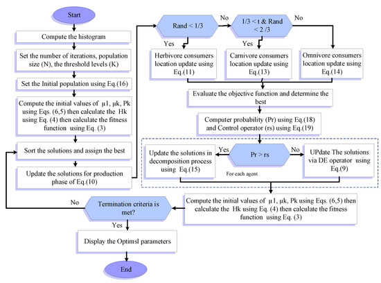
Figure 1. The flowchart of the AEODE.

In general, the developed AEODE begins by using Equation (25) to generate the initial population X as shown in the following equation:

$$X_{i,j}=I_{min,j}+r_1\times (I_{max,j}-I_{min,j}),i=1,2,\dots ,N$$

(25)

In Equation (25), the value of $I_{max,j}$ and $I_{min,j}$ represent the maximum and minimum gray value of I at dimension j, respectively, whereas $Dim=2K$ is the dimension of each solution (here K refers to the threshold levels used to segment I). Therefore, the best solution $X_b$ is allocated, followed by updating the value of other solutions.

The process of updating solutions is implemented, using the operators of the traditional AEO algorithm during the exploration. However, in the case of the solutions that go through the exploitation phase, they will be updated using either the operators of AEO or DE, using the following equation:

$$X_i=\left\{\begin{array}{cc}operatorsofAEO& P{r}_i>r_s\\ operatorsofDE& otherwise\end{array}\right.$$

(26)

In Equation (26), $P{r}_i$ is the probability of each $X_i$ and it depends on the fitness value ($Fi{t}_i$, which is defined in Equation (3). The formulation of $P{r}_i$ is given as follows:

$$P{r}_i=\frac{Fi{t}_i}{{\sum }_{i=1}^{N}Fi{t}_i}$$

(27)

where

$$r_s=min\left(P{r}_i\right)+rand\times (max\left(P{r}_i\right)-min\left(P{r}_i\right)),rand\in [0,1]$$

(28)

The main objective of using $r_s$ is a variable that controls the process of using the operators of DE and AEO. To avoid the problem of making it a constant value since it is expected that the value of $P{r}_i$ is increased with excess iterations, the operators of AEO are used only, especially at the end of iterations. Therefore, we update dynamically the value of $r_s$ according to the probability of each solution. This gives the developed AEODE high flexibility in switching between AEO and DE.

The next process in AEODE is to check the terminal criteria and return by the best solution when they are reached (i.e., here, the maximum number of iterations), followed by extracting the threshold values from $X_b$ as $t_k=\frac{X_b^k+X_b^{k+1}}{2},k=1:2:K-1$.

Complexity of AEODE

The complexity of the AEODE, in general, depends on the complexity of traditional AEO, quick sort (QS), and DE. Since the complexity of DE is given as

$$O\left(DE\right)=O((N\times D+N\times D+N)\times t_{max})$$

(29)

Therefore, the complexity of AEODE is given as follows:

$$O\left(AEODE\right)=O(t_{max}\times (Term1+Term2))$$

(30)

$$Term1=(QS+N\times D+N\times D+N)$$

$$Term2=((N_K\times D+N_K\times D+N_K)+(N-N_K)\times D)$$

In the best case of QS, the complexity of AEODE is given as follows:

$$O\left(AEODE\right)=O\left(t_{max}\times (NlogN+N\times D+N_K\times D+N_K)\right)$$

(31)

In the worst case of QS, the complexity of AEODE is given as follows:

$$O\left(AEODE\right)=O\left(t_{max}\times (N^2+N\times D+N_K\times D+N_K)\right)$$

(32)

where $N_K$ is the number of solutions updated, using DE.

5. Evaluation Experiment

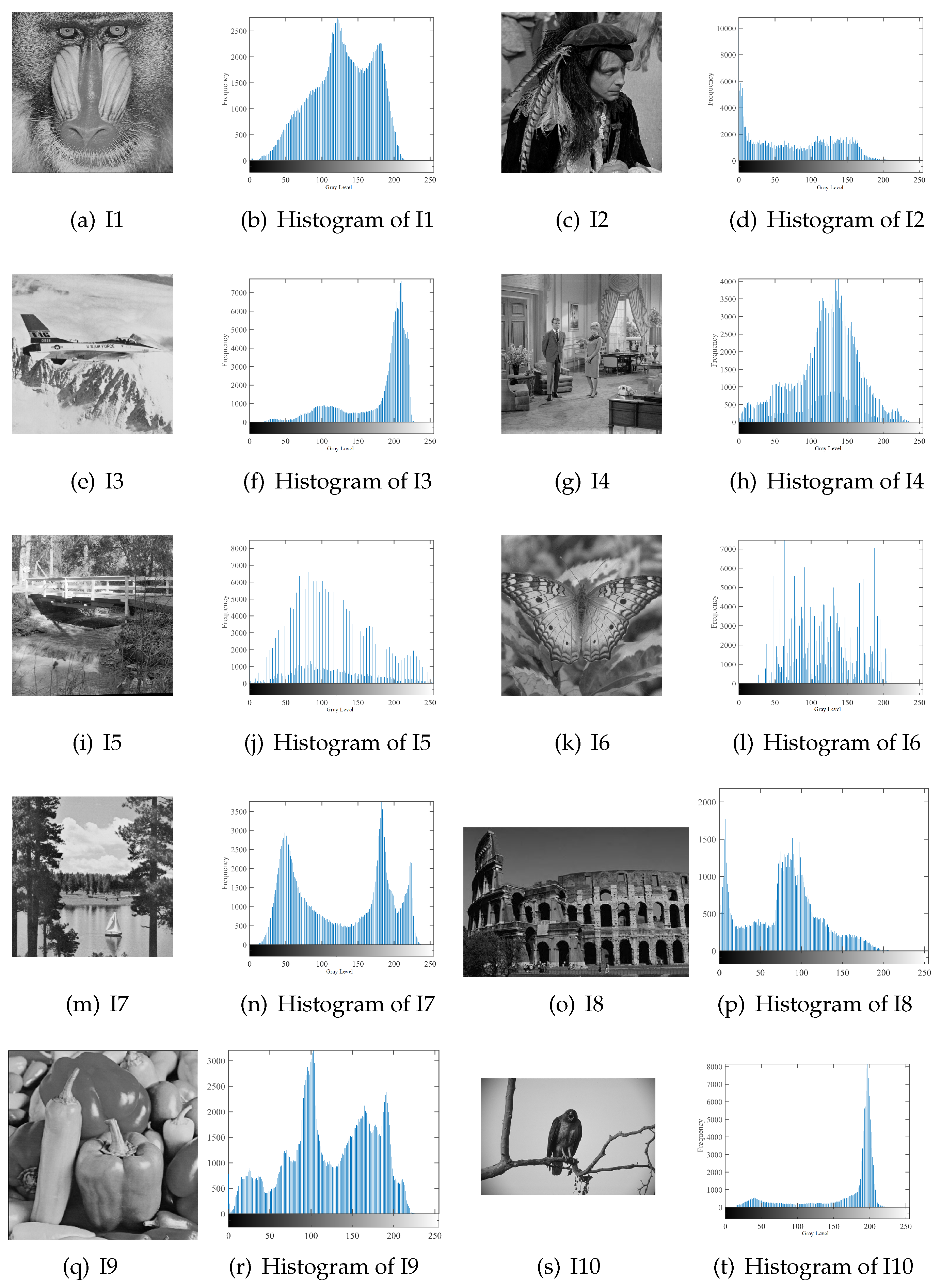
We compare the proposed AEODE method with relevant approaches to segment 10 standard test images, as shown in Figure 2. In addition, the histogram of each image is given in Figure 2 which indicates the characteristic of each image. Swarm parameters are adjusted to their original implementations [28]. The number of population is set to 20, while the dimension equals the threshold level. Moreover, the iteration number is set to 100, and all parameters are selected, depending on the recommendation by the authors of [29].

Figure 2. Tested images with their histograms.

Several threshold values were adopted to test the proposed approach (i.e., 6, 8, 15, 17, 19, and 25). The performance of the AEODE was obtained by applying it on several images that are variant in shape, morphology, and contents. The experiments were implemented, using Matlab 2014b on a computer “Core i5 and 8 GB of RAM running on MS Windows 10”.

5.1. Performance Measures

We evaluate the performance of the AEODE using three performance measures, called the fitness function value, the structural similarity index (SSIM), and the peak signal-to-noise ratio (PSNR). SSIM and PSNR are computed by the following equations:

$$SSIM(I,I_S)=\frac{(2{\mu }_I{\mu }_{I_S}+c_1)(2{\sigma }_{I,I_S}+c_2)}{({\mu }_I^2+{\mu }_{I_S}^2+c_1)({\sigma }_I^2+{\sigma }_{I_S}^2+c_2)}$$

(33)

where ${\mu }_{I_S}$ (${\sigma }_{I_S}$) and ${\mu }_I$(${\sigma }_I$) represent images’ mean intensity of $I_S$ and I, respectively. ${\sigma }_{I,I_S}$ defines the covariance of I and $I_S$. $c_1$ and $c_2$ are equal to 6.5025 and 58.52252, respectively [30].

$$PSNR=20lo{g}_{10}\left(\frac{255}{RMSE}\right),$$

(34)

$$RMSE=\sqrt{\frac{{\sum }_{i=1}^{N_r}{\sum }_{j=1}^{N_c}{(I_{i,j}-I_{S}i,j)}^2}{N_r\times N_c}}$$

where $RMSE$ refers to the root mean-squared error.

5.2. Results and Discussion

The proposed AEODE method is tested besides other optimization algorithms, such as the basic artificial ecosystem-based optimization (AEO), marine predators algorithm (MPA), gray wolf optimization (GWO), spherical search optimization (SSO), cuckoo search (CS), and grasshopper optimization algorithm (GOA). The results can be divided mainly into three main categories, as follows.

5.2.1. Performance Measure by Structural Similarity Index (SSIM)

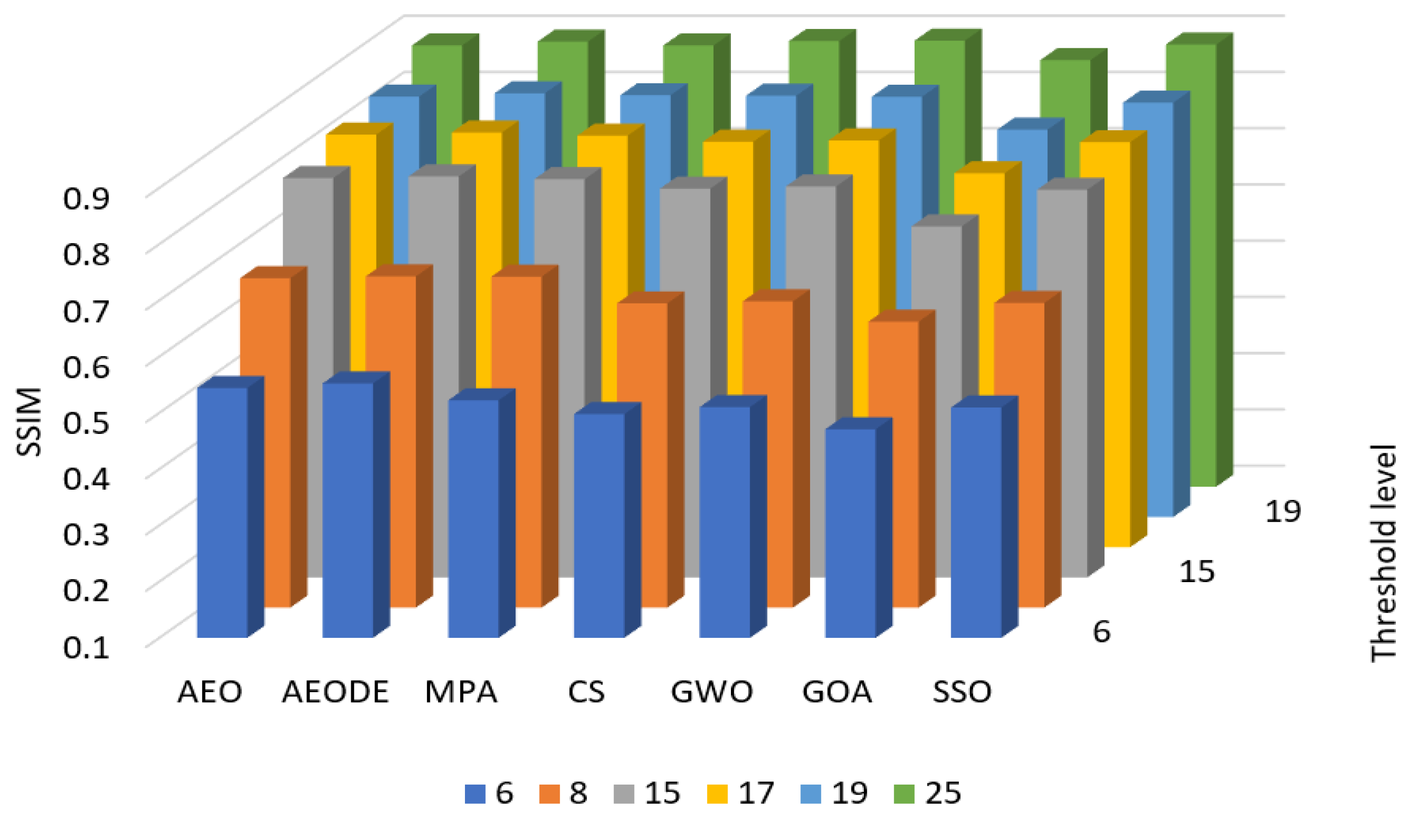
Figure 3 and Table 1 show the results of our AEODE method, compared to the most recent optimization algorithms based on SSIM measure.

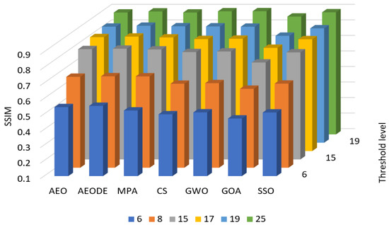
Figure 3. SSIM at different threshold levels.

Table 1. SSIM results for all algorithms (bold means the best value).

Threshold	Image	AEO	AEODE	MPA	CS	GWO	SSA	GOA	SSO
6	I1	0.53396	0.5618	0.50579	0.52352	0.51025	0.39938	0.48972	0.53913
	I2	0.44281	0.43436	0.41918	0.40398	0.40233	0.52873	0.38488	0.40887
	I3	0.6135	0.62192	0.59835	0.61624	0.60716	0.64755	0.61252	0.63662
	I4	0.52059	0.52952	0.48349	0.5448	0.55125	0.52551	0.53858	0.53506
	I5	0.39568	0.4004	0.37672	0.29943	0.31531	0.39835	0.24689	0.35574
	I6	0.4401	0.45909	0.41752	0.3415	0.36174	0.39093	0.30873	0.38448
	I7	0.45267	0.46214	0.4291	0.41906	0.4188	0.54524	0.39571	0.42966
	I8	0.56102	0.56591	0.54474	0.59211	0.57265	0.64572	0.54101	0.57902
	I9	0.7241	0.73382	0.71886	0.57796	0.70238	0.71535	0.56442	0.54372
	I10	0.75823	0.75492	0.73026	0.66034	0.66138	0.77956	0.62704	0.68312
8	I1	0.72614	0.72068	0.71035	0.71459	0.70441	0.54141	0.68052	0.70587
	I2	0.55282	0.56874	0.58633	0.45404	0.45667	0.52761	0.40373	0.46437
	I3	0.72347	0.72196	0.70095	0.76111	0.75279	0.65808	0.75203	0.77642
	I4	0.645	0.65213	0.65855	0.60049	0.58887	0.55473	0.57312	0.60482
	I5	0.63042	0.63415	0.63535	0.55223	0.56527	0.52105	0.53659	0.53372
	I6	0.6327	0.63537	0.6475	0.51139	0.5342	0.41109	0.44601	0.53234
	I7	0.61356	0.61623	0.6379	0.58497	0.56852	0.58721	0.53671	0.58961
	I8	0.72496	0.73439	0.71537	0.64796	0.70713	0.64018	0.63638	0.63361
	I9	0.77189	0.76749	0.77213	0.80557	0.80464	0.74337	0.78055	0.80571
	I10	0.8359	0.83796	0.81993	0.77708	0.76321	0.79199	0.73836	0.76977
15	I1	0.84257	0.84348	0.83516	0.8378	0.81281	0.6043	0.79505	0.83572
	I2	0.70787	0.72741	0.72224	0.67424	0.70364	0.58825	0.58646	0.66409
	I3	0.82551	0.82882	0.78965	0.85413	0.84984	0.7061	0.82652	0.8465
	I4	0.76668	0.76218	0.76217	0.73951	0.74846	0.58438	0.68076	0.76032
	I5	0.80116	0.80893	0.798	0.76274	0.78447	0.55193	0.67289	0.76257
	I6	0.76882	0.76403	0.75681	0.74085	0.72203	0.43352	0.61737	0.75585
	I7	0.76895	0.77076	0.78581	0.76759	0.79293	0.61501	0.64608	0.76416
	I8	0.84272	0.83542	0.84811	0.8248	0.83539	0.68349	0.76642	0.82585
	I9	0.86649	0.87485	0.8676	0.84894	0.8542	0.8011	0.82481	0.83208
	I10	0.90939	0.91455	0.9152	0.86198	0.84617	0.81927	0.82345	0.84518
17	I1	0.86894	0.86292	0.85717	0.87164	0.8434	0.59045	0.83058	0.86417
	I2	0.7478	0.76251	0.75533	0.73452	0.75615	0.54872	0.61554	0.72061
	I3	0.84686	0.83269	0.82665	0.86869	0.86657	0.72056	0.85029	0.87188
	I4	0.78076	0.80353	0.79274	0.77364	0.77225	0.56542	0.72636	0.77225
	I5	0.83757	0.84195	0.83266	0.81014	0.82748	0.60601	0.74483	0.80114
	I6	0.79235	0.79536	0.78603	0.77734	0.77474	0.47968	0.67667	0.80482
	I7	0.80524	0.81419	0.79872	0.78759	0.81934	0.62238	0.72879	0.7812
	I8	0.86742	0.87129	0.87037	0.84137	0.8635	0.68178	0.79223	0.85152
	I9	0.86965	0.87394	0.87281	0.85917	0.85488	0.8118	0.83079	0.85502
	I10	0.91904	0.91465	0.92399	0.88497	0.85498	0.83222	0.85329	0.87835
19	I1	0.87635	0.88501	0.87613	0.883	0.86528	0.59886	0.84743	0.88062
	I2	0.76872	0.77978	0.78149	0.7644	0.78806	0.59244	0.66842	0.74173
	I3	0.85051	0.84382	0.83837	0.87621	0.87408	0.69963	0.85775	0.87997
	I4	0.81724	0.83029	0.82357	0.79278	0.80193	0.55642	0.73432	0.78558
	I5	0.86194	0.86551	0.84376	0.85091	0.85249	0.57686	0.78763	0.82448
	I6	0.81372	0.81319	0.81469	0.8361	0.80929	0.49202	0.71495	0.81491
	I7	0.82006	0.82438	0.83027	0.83388	0.84005	0.64693	0.76148	0.82062
	I8	0.87385	0.88711	0.87839	0.87664	0.88092	0.72755	0.80646	0.86929
	I9	0.88497	0.88746	0.88334	0.87026	0.87113	0.81153	0.83718	0.86986
	I10	0.90722	0.91623	0.92831	0.90501	0.88699	0.82973	0.87028	0.87877
25	I1	0.91122	0.91809	0.91088	0.91508	0.90582	0.64155	0.8951	0.91449
	I2	0.82578	0.83129	0.82393	0.83724	0.8647	0.63701	0.79231	0.8200
	I3	0.86761	0.88327	0.88309	0.90407	0.90137	0.7196	0.88303	0.89804
	I4	0.86909	0.87565	0.85928	0.86056	0.85436	0.60861	0.82264	0.85181
	I5	0.90929	0.91231	0.90371	0.91259	0.91112	0.60574	0.86639	0.89367
	I6	0.86516	0.87165	0.86501	0.87474	0.88643	0.57681	0.82227	0.8918
	I7	0.86834	0.87462	0.86578	0.87983	0.87767	0.66865	0.84386	0.87017
	I8	0.91503	0.91964	0.91417	0.9118	0.91455	0.75603	0.88377	0.90359
	I9	0.90205	0.90818	0.90161	0.90348	0.8934	0.81819	0.87403	0.89324
	I10	0.91263	0.91849	0.91732	0.92418	0.92226	0.8431	0.9025	0.92624

Figure 3 shows that the AEODE performs better in both of the low thresholding levels (i.e., 5 and 6) and also in the higher thresholding levels (i.e., 19 and 25), while GOA shows the lowest performance among other optimization algorithms.

Table 1 shows the SSIM values performed by each optimization algorithm for each image with different threshold levels. From Table 1, we see that the AEODE method allocates the first rank (the highest SSIM values at 25 cases), followed by MPA and CS algorithms (eight highest SSIM values for each), which provide better results than others. Additionally, AEODE achieved good SSIM values in all threshold levels.

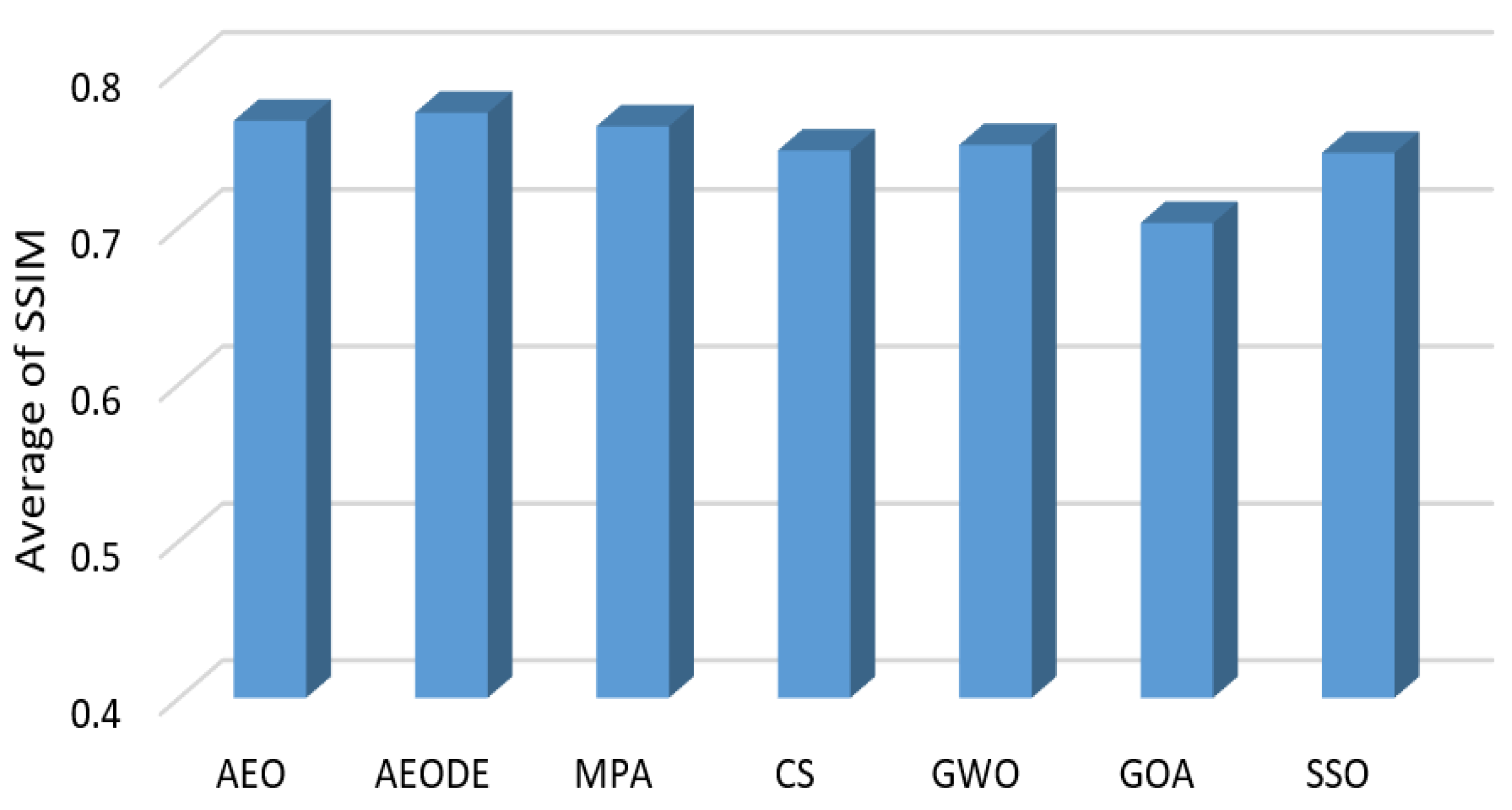
Figure 4 summarizes the average SSIM values with different threshold levels. From Figure 4, we notice that the AEODE outperforms other algorithms, such as AEO, MPA, CS, GWO, GOA, and SSO, by achieving the highest average of SSIM with different threshold levels, with a slight advantage over MPA and SSO.

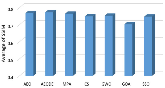
Figure 4. Average SSIM values for all algorithms’ overall images.

5.2.2. Performance Measure by Peak Signal-to-Noise Ratio (PSNR)

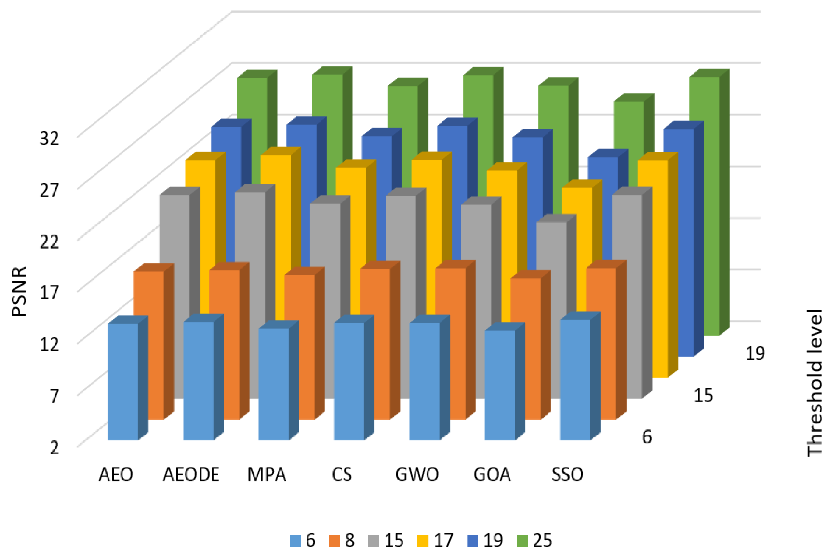
Table 2 and Figure 5 present the performance of the AEODE, compared to other recent optimization algorithms based on PSNR measured with different threshold values.

Table 2. PSNR results for all algorithms (bold means the best value).

Threshold	Image	AEO	AEODE	MPA	CS	GWO	GOA	SSO
6	I1	14.3825	14.8805	14.0022	14.2535	14.123	13.5623	14.5985
	I2	16.776	16.5781	16.25	15.8815	15.6123	15.4548	15.9642
	I3	10.301	10.4584	10.0393	12.8807	12.6054	11.3303	13.4835
	I4	15.5356	15.6956	14.7613	16.2105	16.3312	16.0247	16.0098
	I5	13.002	13.0219	12.7031	11.6661	11.9035	10.8805	12.5634
	I6	13.8393	14.1526	13.4173	11.9244	12.183	11.5066	12.6031
	I7	12.1668	12.2929	11.7442	11.983	11.8217	11.6867	12.3337
	I8	13.8981	13.9791	13.5196	14.4894	14.0186	13.3968	14.1717
	I9	11.5561	12.0803	11.0956	10.1514	10.5988	9.38632	10.1912
	I10	11.394	11.3348	10.7158	14.212	14.4238	13.0733	14.7021
8	I1	18.0812	18.0815	17.6837	18.1512	17.7062	17.0512	18.1623
	I2	19.713	19.895	20.1166	16.8944	16.5392	15.6426	17.0666
	I3	12.554	12.6388	11.8524	15.7199	15.9636	14.909	16.5606
	I4	18.3923	18.567	18.5216	17.6977	17.0637	16.7765	17.7364
	I5	16.5871	16.7741	16.2219	16.0126	16.1572	15.7477	15.7234
	I6	17.726	17.9671	18.0062	15.1837	15.5847	14.0664	15.7411
	I7	14.8103	14.9134	14.6142	15.9958	15.5439	15.1388	16.2394
	I8	17.7434	18.0346	17.2219	15.1528	16.8989	14.7088	15.0617
	I9	13.7439	13.7056	12.8298	15.5042	15.4239	14.2372	15.6629
	I10	13.6444	13.8088	12.5811	19.1078	19.316	18.1821	18.3384
15	I1	22.9214	22.977	22.2853	23.0132	21.5091	20.8354	22.8682
	I2	23.5558	23.861	23.5189	22.437	22.187	20.0346	22.4572
	I3	19.1193	19.4112	16.7735	21.5282	19.6672	19.2986	21.9266
	I4	22.3949	22.249	22.0038	21.6674	21.6847	19.8822	22.5474
	I5	21.7982	22.1718	21.3887	21.1647	21.2952	18.609	21.1493
	I6	22.6571	22.4339	21.9557	21.1505	20.3099	17.7507	21.9507
	I7	21.2712	22.3375	20.2573	21.3237	20.229	18.4218	21.5466
	I8	22.219	22.1627	22.2886	21.8225	21.2988	18.7217	21.6013
	I9	20.1963	20.8863	18.9355	20.9695	18.0963	17.7748	19.9499
	I10	21.2212	21.558	19.7074	21.4588	21.4665	19.492	21.4161
17	I1	24.0811	23.8706	23.5962	24.5295	23.0746	22.3151	24.2334
	I2	24.7625	25.1301	24.5872	24.1457	24.0483	20.8547	23.8381
	I3	20.8615	21.862	19.2265	23.327	20.6577	20.9033	23.3563
	I4	22.9854	23.9083	23.2481	22.8942	22.4866	20.9846	22.8827
	I5	23.4436	23.4242	22.3991	22.6849	22.8679	20.3653	22.2991
	I6	23.6858	23.9178	23.1132	22.2126	22.1551	19.2307	23.9446
	I7	23.0405	23.2971	21.5097	22.6135	21.4138	20.1451	22.1639
	I8	23.5485	23.847	23.4845	22.6809	22.8869	19.9435	23.2374
	I9	21.3322	22.7893	20.6068	22.7039	19.356	18.9158	21.635
	I10	22.9969	23.5863	21.6966	23.1547	21.9301	20.5416	23.0256
19	I1	24.4745	25.1133	24.517	25.2359	24.251	23.0769	25.1513
	I2	25.6186	25.4214	25.5213	25.35	24.9708	22.2735	24.5691
	I3	22.5205	23.8711	20.6197	24.743	21.7863	21.5832	25.1239
	I4	24.6237	25.2183	24.561	23.7095	23.9133	21.4378	23.342
	I5	24.2058	24.3305	23.3839	24.1541	23.8568	21.7525	23.1785
	I6	24.6762	24.7183	24.4006	24.8508	23.6233	20.3269	24.0407
	I7	23.6407	23.9977	23.3394	24.5317	22.6665	21.2738	24.2728
	I8	23.8093	24.8603	24.0163	24.1517	23.8789	20.4655	24.1552
	I9	24.225	22.7931	21.2062	22.5229	20.8636	19.7875	22.4684
	I10	24.7213	24.4432	22.0929	24.3168	22.7555	21.4517	24.1257
25	I1	26.9248	27.4147	26.7551	27.4008	26.7323	25.7589	27.4094
	I2	27.912	28.2136	27.5864	28.2266	28.058	26.214	27.7472
	I3	26.8428	27.1681	24.4243	26.8027	23.9304	23.9079	27.4464
	I4	27.1151	27.5947	26.5531	26.7518	26.2573	24.955	26.3363
	I5	26.8594	27.1087	26.1684	27.3946	26.9059	24.8264	26.3298
	I6	27.1197	27.4133	26.8836	26.7446	27.1805	23.7763	28.3197
	I7	26.7169	27.0784	25.6628	27.4061	25.9714	24.7308	26.7924
	I8	27.1753	27.3743	26.6731	27.2032	26.7091	24.6398	26.6686
	I9	25.9341	26.2033	24.8043	26.5647	24.4355	23.3068	25.7296
	I10	26.8821	27.2701	26.1785	27.6637	25.9562	24.6613	27.6004

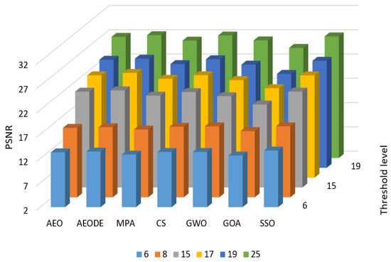
Figure 5. PSNR at different threshold levels.

It can be noticed from Figure 3 that the proposed AEODE outperforms other optimization algorithms at most threshold levels (except at level 8). Table 2 shows the PSNR values performed by the proposed method and other optimization algorithms for each image with all threshold levels.

From Table 2, it is noticed that the proposed AEODE method allocates the first rank with the highest PSNR values at 23 cases, while SSO and CS are in second and third ranks with the highest 13 and 12 PSNR values, respectively. According to Table 2, the proposed AEODE method performs better with higher thresholding levels (at level 17 and higher) than lower levels.

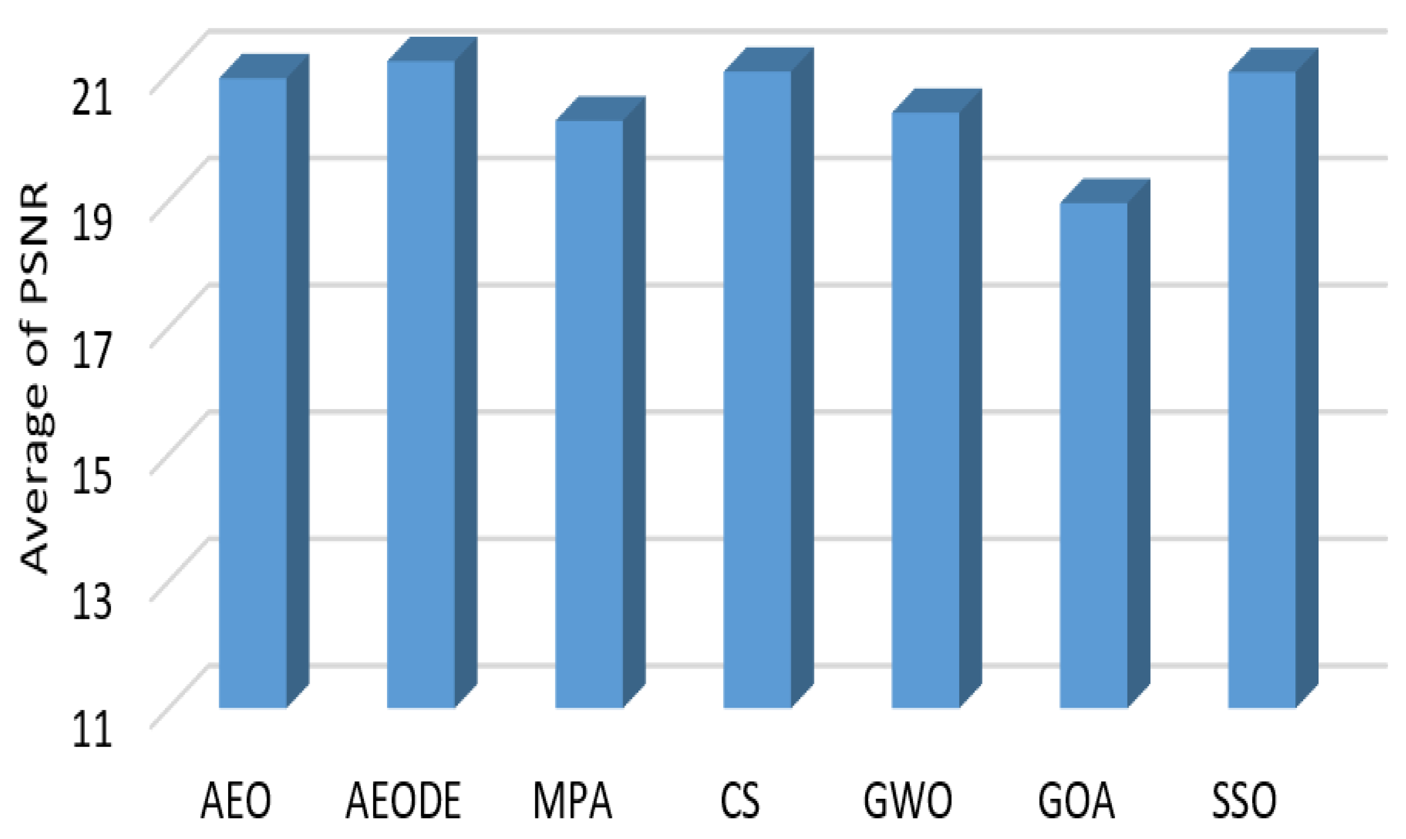
Figure 6 summarizes the average PSNR values with all threshold levels. Figure 6 shows that our proposed method outperforms other optimization algorithms by achieving the highest average of PSNR with different threshold levels for all images. GOA achieves the worst performance, putting it last.

Figure 6. PSNR values of AEODE and other optimization algorithms.

5.2.3. Performance Measure by Fitness Function

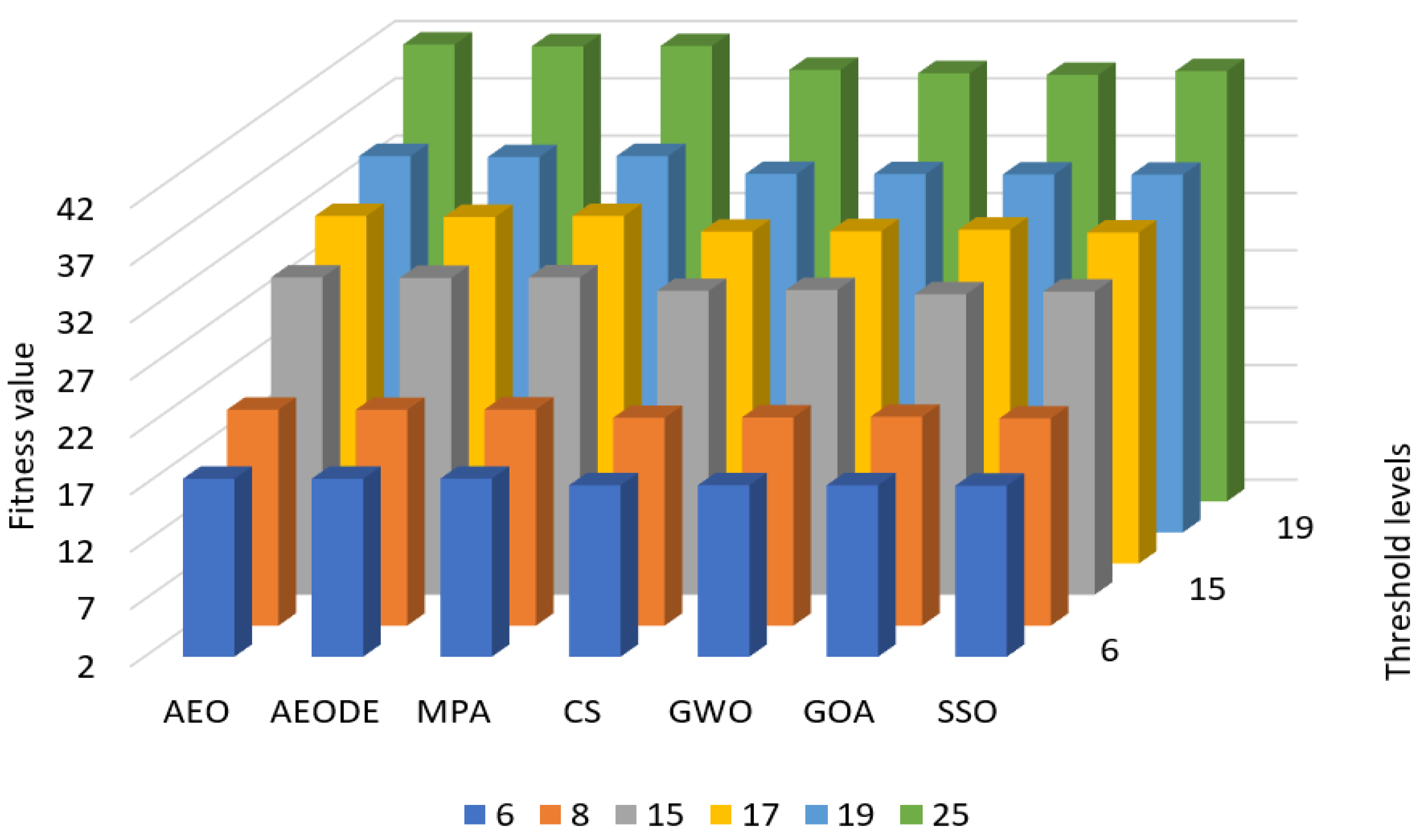
Figure 7 and Table 3 show the fitness function values of AEODE method and other optimization algorithms with different threshold levels.

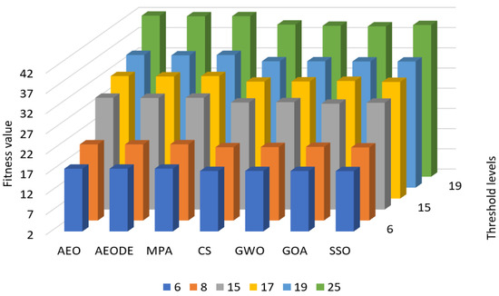
Figure 7. Fitness values of AEODE and other optimization algorithms.

Table 3. Fitness function results for all algorithms (bold means the best value).

Threshold	Image	AEO	AEODE	MPA	CS	GWO	SSA	GOA	SSO
6	I1	17.5265	17.5167	17.5348	17.5163	17.5245	14.555	17.5398	17.4546
	I2	17.5215	17.5209	17.5372	17.2918	17.2894	15.5694	17.3161	17.2726
	I3	17.5249	17.52	17.5372	17.0874	17.0818	13.9699	17.1016	17.0616
	I4	17.5298	17.5217	17.5364	17.5522	17.5704	15.3916	17.5896	17.5283
	I5	17.5273	17.5211	17.5362	15.5982	15.5925	12.7276	15.6182	15.6395
	I6	17.531	17.5214	17.5366	15.0703	15.0806	11.5213	15.1272	15.0172
	I7	17.5305	17.5192	17.5379	17.6206	17.6236	15.135	17.3165	17.4764
	I8	17.5323	17.5327	17.5334	17.5738	17.5903	15.4892	17.6009	17.5415
	I9	17.5272	17.5201	17.5359	17.4772	17.5094	14.9546	17.5371	17.4722
	I10	17.5233	17.5177	17.5364	16.7679	16.7749	14.0574	16.7988	16.7677
8	I1	20.8258	20.8222	20.8474	20.7724	20.8195	15.6432	20.8393	20.6894
	I2	20.8179	20.818	20.8467	20.7772	20.8182	16.2007	20.914	20.6923
	I3	20.8335	20.8203	20.8516	20.443	20.4538	14.4673	20.5345	20.3825
	I4	20.8315	20.8183	20.8546	20.9136	20.9509	16.3078	21.0092	20.8526
	I5	20.8266	20.816	20.8484	18.2622	18.322	14.1362	18.3769	18.2611
	I6	20.8341	20.8238	20.8486	17.3866	17.4261	11.5681	17.5021	17.2807
	I7	20.8299	20.8306	20.8422	20.8701	20.9101	15.3929	20.9493	20.8268
	I8	20.842	20.8136	20.8474	20.8738	20.8353	15.306	20.9881	20.8589
	I9	20.8349	20.8287	20.8386	20.9832	21.0398	15.6711	21.0546	20.9873
	I10	20.826	20.8282	20.8418	19.9763	20.0173	14.7812	20.0601	19.9178
15	I1	29.6442	29.6133	29.6279	29.3907	29.4684	16.2101	29.8008	29.2784
	I2	29.6674	29.6322	29.6724	29.6823	29.7556	16.0706	28.5566	29.6875
	I3	29.6503	29.5867	29.5937	29.2606	29.2624	14.0884	28.5465	29.131
	I4	29.6753	29.5881	29.6813	29.5308	29.6343	15.9021	30.0178	29.5538
	I5	29.6461	29.6588	29.6368	25.204	25.2145	13.7662	25.7182	25.2165
	I6	29.6671	29.6193	29.6527	23.6303	23.6167	11.6248	24.2313	23.1818
	I7	29.6416	29.6049	29.6934	29.4742	29.5973	14.9086	28.6135	29.4155
	I8	29.6577	29.6269	29.6843	30.0662	30.1392	15.5166	28.6444	30.0349
	I9	29.6793	29.6249	29.6955	29.748	30.0096	15.2901	28.5204	29.9023
	I10	29.6519	29.5961	29.6896	28.8684	28.9454	14.781	29.281	28.8635
17	I1	32.3488	32.2296	32.3095	31.9577	31.9444	16.0424	31.0762	31.8416
	I2	32.2875	32.2371	32.3061	32.3915	32.4331	15.7114	33.0069	32.4197
	I3	32.3439	32.214	32.3012	31.7861	31.7911	15.0282	32.4284	31.6946
	I4	32.2961	32.2027	32.2791	32.1339	32.1396	16.4578	32.7554	32.1749
	I5	32.3251	32.2187	32.3283	27.1632	27.2144	13.1787	27.7373	27.2223
	I6	32.3018	32.1828	32.2808	25.2824	25.287	11.5259	26.1223	24.6364
	I7	32.2647	32.2341	32.3332	32.1072	32.1944	15.0693	32.6285	32.099
	I8	32.3107	32.215	32.3415	32.6783	32.71	15.2613	33.3399	32.6571
	I9	32.347	32.2675	32.2917	32.4441	32.5326	14.957	30.9936	32.4632
	I10	32.3163	32.1987	32.3126	31.4601	31.5808	14.6868	31.0726	31.5033
19	I1	34.8139	34.8003	34.8714	34.3638	34.2342	16.3417	33.2823	34.2175
	I2	34.8117	34.7727	34.8053	34.9751	34.9733	16.3809	33.3096	35.0698
	I3	34.8028	34.6484	34.7831	34.2196	34.14	14.9697	35.0649	34.0982
	I4	34.8114	34.7633	34.8187	34.6671	34.6481	15.7964	35.3929	34.6825
	I5	34.8495	34.7301	34.826	28.9961	29.036	13.6795	29.684	29.1493
	I6	34.8331	34.7356	34.8254	26.7512	26.5405	11.5293	27.536	25.9821
	I7	34.82	34.7292	34.8609	34.6364	34.73	15.3604	35.3216	34.5569
	I8	34.808	34.7364	34.799	35.2033	35.228	15.4885	35.9805	35.2658
	I9	34.8603	34.7427	34.8427	34.9619	35.0218	15.9977	33.319	35.0619
	I10	34.8632	34.768	34.8505	33.9221	34.0155	15.1945	33.3191	34.0152
25	I1	41.8453	41.7239	41.6587	41.0703	40.6435	17.1863	39.5637	40.9583
	I2	41.8725	41.6996	41.7333	42.1871	41.8686	16.6713	42.9219	42.1336
	I3	41.8546	41.756	41.7622	40.6073	40.2479	15.2268	41.681	40.417
	I4	41.8022	41.6242	41.7986	41.5551	41.2241	17.3623	42.4607	41.6875
	I5	41.8499	41.7091	41.724	33.8368	33.7225	14.7999	34.7461	33.9924
	I6	41.8209	41.6941	41.7224	30.4701	29.6229	12.2152	32.0503	29.2935
	I7	41.8718	41.7143	41.6714	41.5924	41.4857	16.0446	39.5462	41.5544
	I8	41.8436	41.6505	41.671	42.3413	42.1102	16.375	39.7254	42.3516
	I9	41.8299	41.632	41.6478	41.8899	41.9941	16.2916	39.5576	42.1339
	I10	41.8737	41.7306	41.7884	40.8165	40.4964	15.9225	39.7665	40.7734

Based on Figure 7, the proposed AEODE method outperforms other optimization algorithms in all threshold levels, while GOA shows the lowest fitness values in all threshold levels.

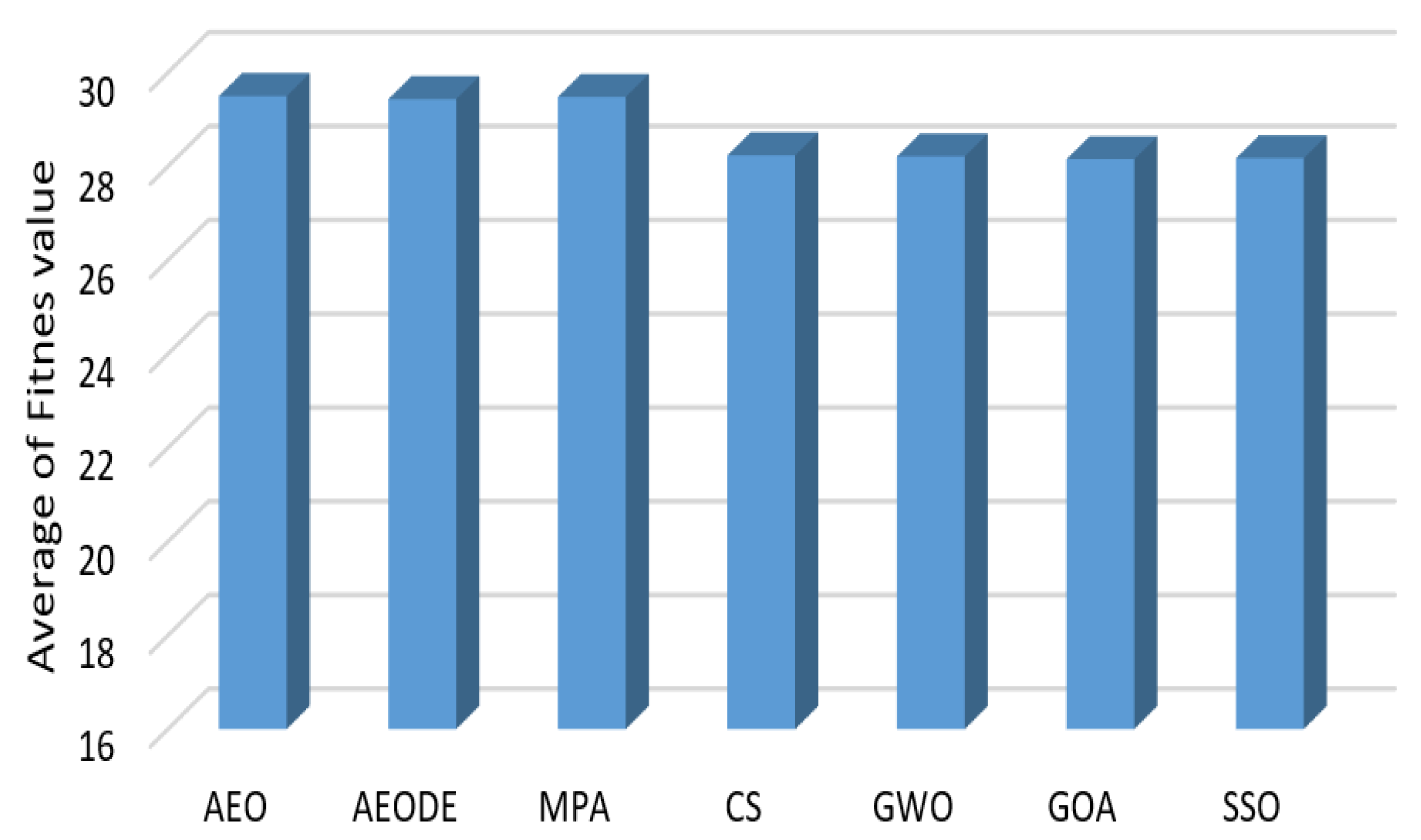
Table 3 shows that all optimization algorithms achieve acceptable fitness values with all threshold levels. There is a slight advantage (in decimal levels) between each one. All optimization algorithms achieve higher fitness values along with higher thresholding levels. The higher the thresholding value, the better the fitness value obtained. Applying the 6, 8, 15, 17, 19, and 25 threshold levels achieves fitness values of 17, 20, 29, 32, 34, and 41, respectively. Figure 8 summarizes the average fitness values with all threshold levels. Based on Figure 8, AEODE, MPA, and AEO came in the first, second, and third ranks, respectively, while GOA is ranked last.

Figure 8. Average fitness values of AEODE and other optimization algorithms.

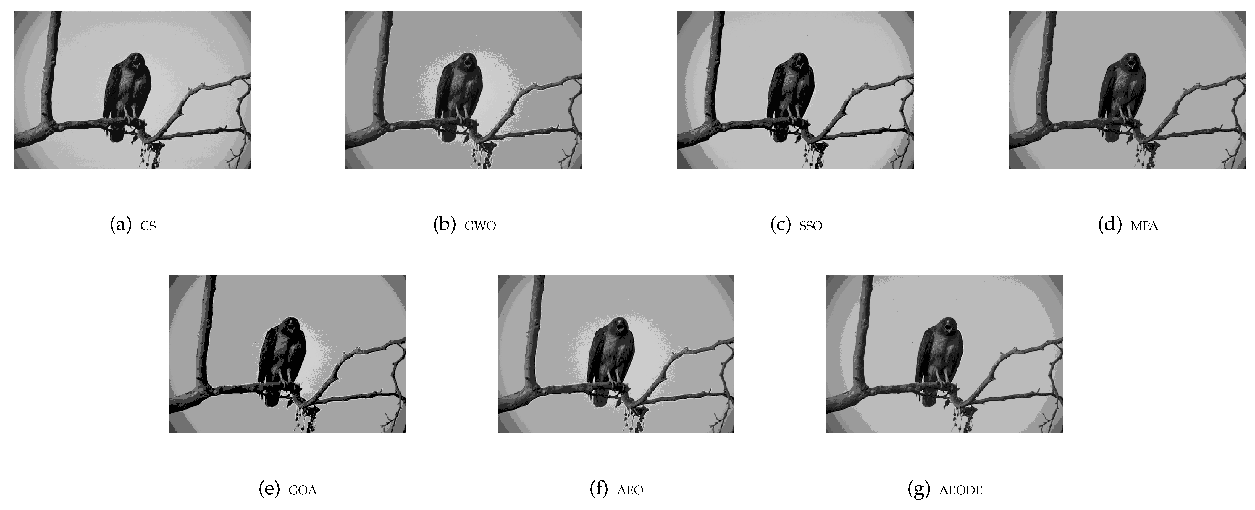
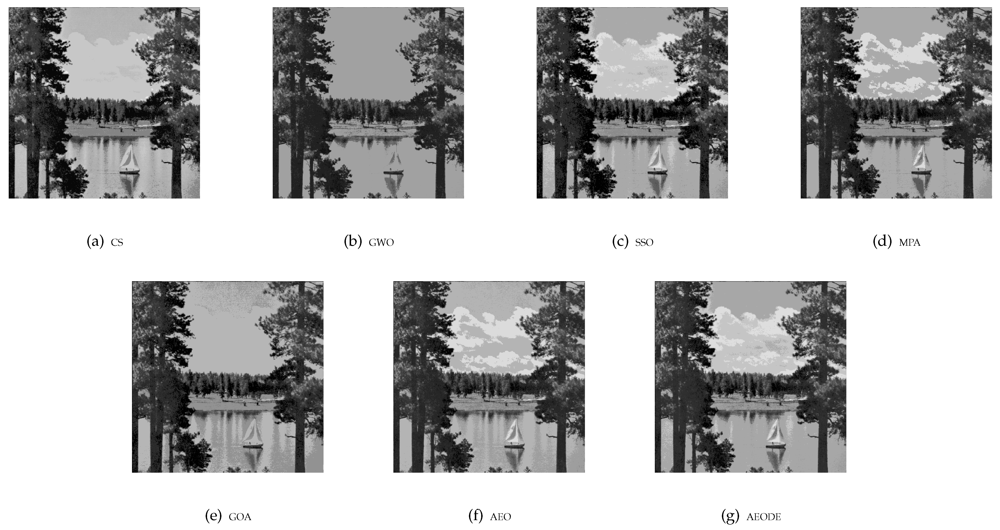
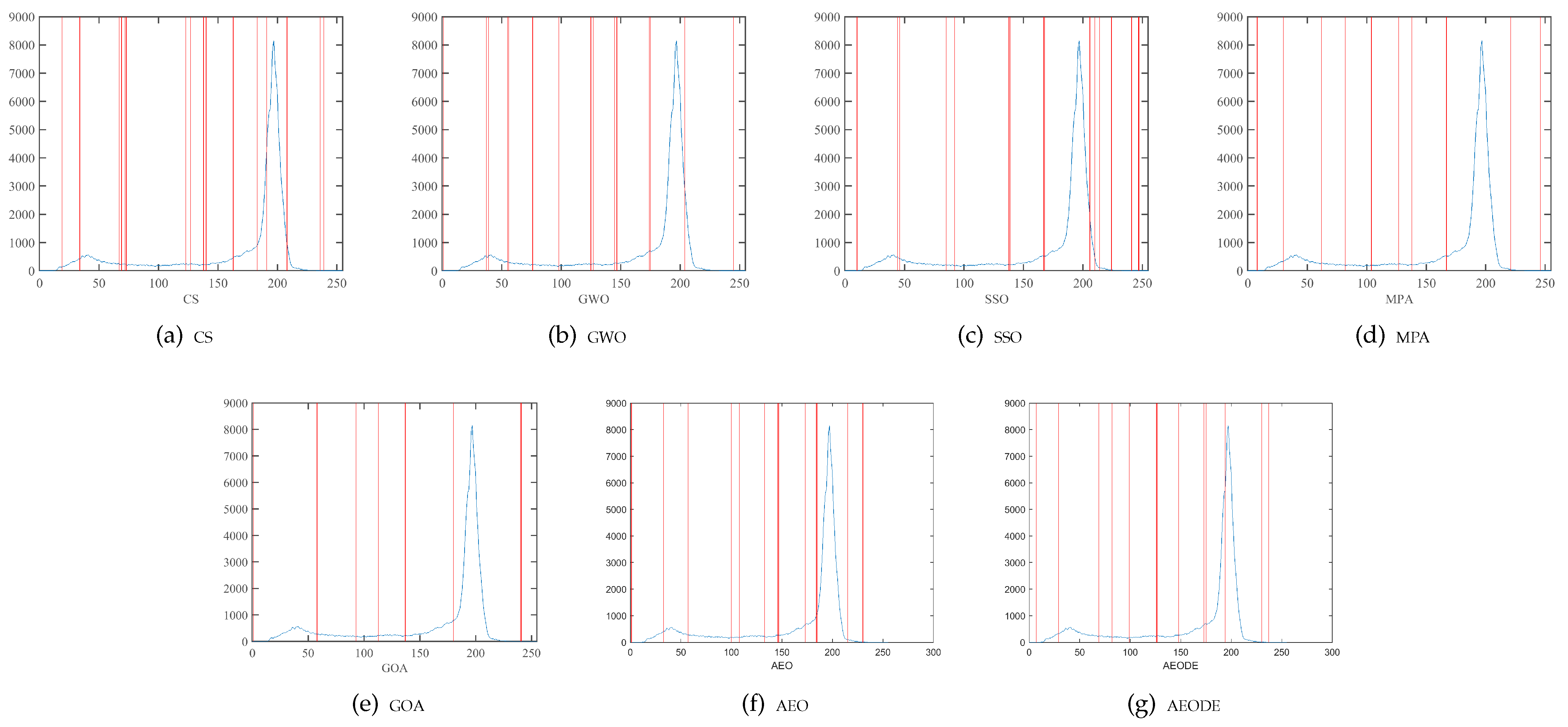
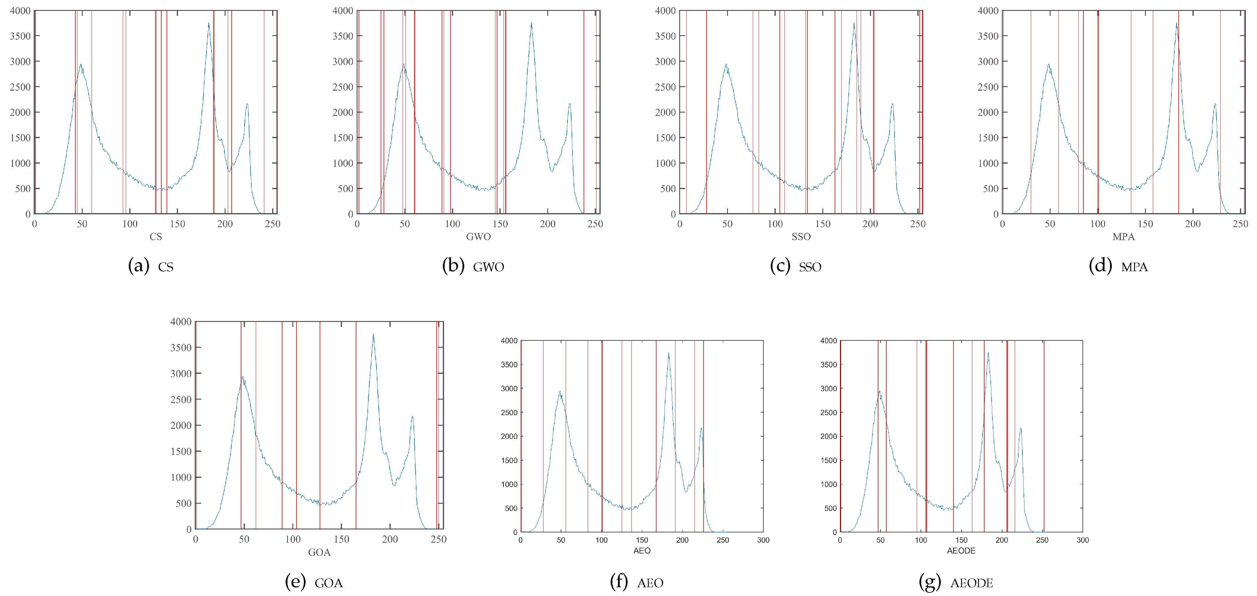
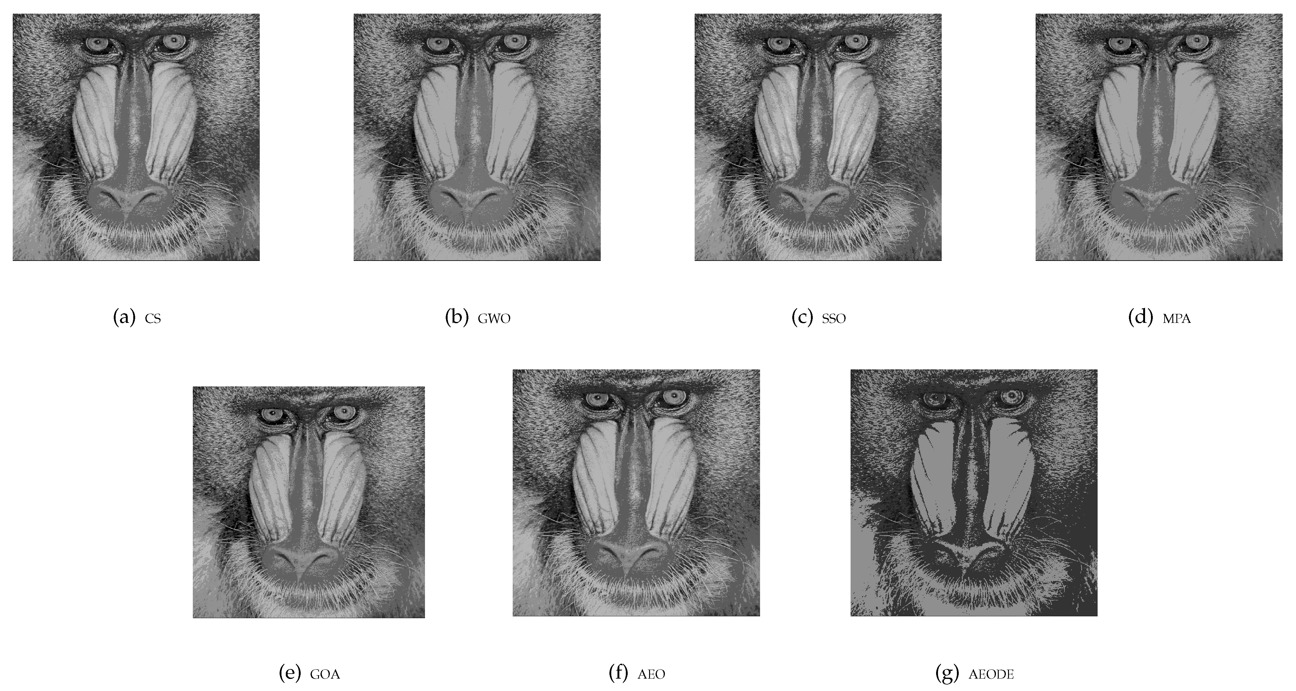
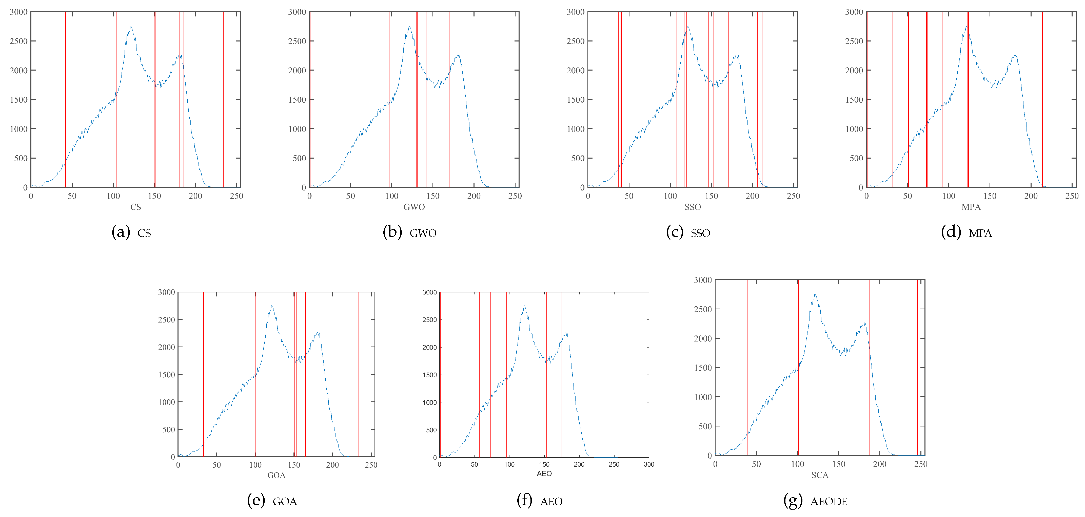
Figure 9 and Figure 10 show the segmented image I10 and image I7, respectively, while their histograms at threshold value 19 are given in Figure 11 and Figure 12 respectively. Both figures show that the proposed method has successfully determined the best threshold value to segment several types of images. Moreover, Figure 13 illustrates the quality of segmented image I1 at level 19. It can be noticed from this figure that the quality of AEODE is decreased in this case since its obtained threshold values do not cover the whole search space (as shown in Figure 14) and its feasible region does not contain the optimal threshold values, which affects the performance of the final output.

Figure 9. Segmentation results at threshold level 19 for the images I10.

Figure 10. Segmented image I7 at threshold level 19.

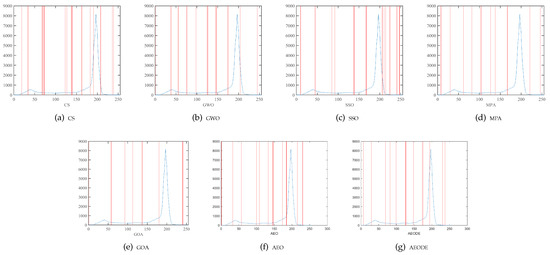
Figure 11. The threshold values at level 19 over the histogram of I10.

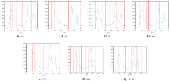
Figure 12. The threshold values at level 19 over the histogram of image I7.

Figure 13. Segmented image I1 at threshold level 19.

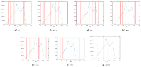
Figure 14. The threshold values at level 19 over the histogram of image I1.

Moreover, the improvement rate between the proposed method and other methods according to each performance measure is computed as follows:

$$IR(\%)=\frac{(S-S^{\prime })}{S^{\prime }}\ast 100$$

(35)

where $S^{\prime }$ and S denote the values obtained by AEODE and values obtained by other methods, respectively.

Table 4 shows the IR for the three measures (i.e., PSNR, SSIM, and fitness value). From this table, it can be noticed that AEODE provides a high IR rate in terms of PSNR, which is better than AEO, MPA, CS, GWO, GOA, and SSO with 47, 46, 44, 44, 55, and 46. In terms of SSIM as well, it provides results better than AEO, MPA, CS, GWO, GOA, and SSO with 49, 56, 37, 51, 53, and 39. However, the IR of the developed AEODE in terms of the fitness value is better than AEO and MPA with only 5 and 3 cases. However, with other methods, it still provides better fitness values of 41, 37, 37, and 42 for CS, GWO, GOA, and SSO.

Table 4. Improvement ratio for developed method with other methods (bold means the best value).

		PSNR						SSIM						Fitness
T	I	AEO	MPA	CS	GWO	GOA	SSO	AEO	MPA	CS	GWO	GOA	SSO	AEO	MPA	CS	GWO	GOA	SSO
6	I1	−5.0	−10.0	−6.8	−9.2	−12.8	−4.0	−3.3	−5.9	−4.2	−5.1	−8.9	−1.9	0.1	0.1	−0.0	0.0	0.1	−0.4
	I2	1.9	−3.5	−7.0	−7.4	−11.4	−5.9	1.2	−2.0	−4.2	−5.8	−6.8	−3.7	0.0	0.1	−1.3	−1.3	−1.2	−1.4
	I3	−1.4	−3.8	−0.9	−2.4	−1.5	2.4	−1.5	−4.0	23.2	20.5	8.3	28.9	0.0	0.1	−2.5	−2.5	−2.4	−2.6
	I4	−1.7	−8.7	2.9	4.1	1.7	1.0	−1.0	−6.0	3.3	4.0	2.1	2.0	0.0	0.1	0.2	0.3	0.4	0.0
	I5	−1.2	−5.9	−25.2	−21.3	−38.3	−11.2	−0.2	−2.4	−10.4	−8.6	−16.4	−3.5	0.0	0.1	−11.0	−11.0	−10.9	−10.7
	I6	−4.1	−9.1	−25.6	−21.2	−32.8	−16.3	−2.2	−5.2	−15.7	−13.9	−18.7	−10.9	0.1	0.1	−14.0	−13.9	−13.7	−14.3
	I7	−2.0	−7.1	−9.3	−9.4	−14.4	−7.0	−1.0	−4.5	−2.5	−3.8	−4.9	0.3	0.1	0.1	0.6	0.6	−1.2	−0.2
	I8	−0.9	−3.7	4.6	1.2	−4.4	2.3	−0.6	−3.3	3.7	0.3	−4.2	1.4	−0.0	0.0	0.2	0.3	0.4	0.1
	I9	−1.3	−2.0	−21.2	−4.3	−23.1	−25.9	−4.3	−8.2	−16.0	−12.3	−22.3	−15.6	0.0	0.1	−0.2	−0.1	0.1	−0.3
	I10	0.4	−3.3	−12.5	−12.4	−16.9	−9.5	0.5	−5.5	25.4	27.3	15.3	29.7	0.0	0.1	−4.3	−4.2	−4.1	−4.3
8	I1	0.8	−1.4	−0.8	−2.3	−5.6	−2.1	−0.0	−2.2	0.4	−2.1	−5.7	0.4	0.0	0.1	−0.2	−0.0	0.1	−0.6
	I2	−2.8	3.1	−20.2	−19.7	−29.0	−18.4	−0.9	1.1	−15.1	−16.9	−21.4	−14.2	−0.0	0.1	−0.2	0.0	0.5	−0.6
	I3	0.2	−2.9	5.4	4.3	4.2	7.5	−0.7	−6.2	24.4	26.3	18.0	31.0	0.1	0.2	−1.8	−1.8	−1.4	−2.1
	I4	−1.1	1.0	−7.9	−9.7	−12.1	−7.3	−0.9	−0.2	−4.7	−8.1	−9.6	−4.5	0.1	0.2	0.5	0.6	0.9	0.2
	I5	−0.6	0.2	−12.9	−10.9	−15.4	−15.8	−1.1	−3.3	−4.5	−3.7	−6.1	−6.3	0.1	0.2	−12.3	−12.0	−11.7	−12.3
	I6	−0.4	1.9	−19.5	−15.9	−29.8	−16.2	−1.3	0.2	−15.5	−13.3	−21.7	−12.4	0.0	0.1	−16.5	−16.3	−16.0	−17.0
	I7	−0.4	3.5	−5.1	−7.7	−12.9	−4.3	−0.7	−2.0	7.3	4.2	1.5	8.9	−0.0	0.1	0.2	0.4	0.6	−0.0
	I8	−1.3	−2.6	−11.8	−3.7	−13.3	−13.7	−1.6	−4.5	−16.0	−6.3	−18.4	−16.5	0.1	0.2	0.3	0.1	0.8	0.2
	I9	0.6	0.6	5.0	4.8	1.7	5.0	0.3	−6.4	13.1	12.5	3.9	14.3	0.0	0.0	0.7	1.0	1.1	0.8
	I10	−0.2	−2.2	−7.3	−8.9	−11.9	−8.1	−1.2	−8.9	38.4	39.9	31.7	32.8	−0.0	0.1	−4.1	−3.9	−3.7	−4.4
15	I1	−0.1	−1.0	−0.7	−3.6	−5.7	−0.9	−0.2	−3.0	0.2	−6.4	−9.3	−0.5	0.1	0.0	−0.8	−0.5	0.6	−1.1
	I2	−2.7	−0.7	−7.3	−3.3	−19.4	−8.7	−1.3	−1.4	−6.0	−7.0	−16.0	−5.9	0.1	0.1	0.2	0.4	−3.6	0.2
	I3	−0.4	−4.7	3.1	2.5	−0.3	2.1	−1.5	−13.6	10.9	1.3	−0.6	13.0	0.2	0.0	−1.1	−1.1	−3.5	−1.5
	I4	0.6	−0.0	−3.0	−1.8	−10.7	−0.2	0.7	−1.1	−2.6	−2.5	−10.6	1.3	0.3	0.3	−0.2	0.2	1.5	−0.1
	I5	−1.0	−1.4	−5.7	−3.0	−16.8	−5.7	−1.7	−3.5	−4.5	−4.0	−16.1	−4.6	−0.0	−0.1	−15.0	−15.0	−13.3	−15.0
	I6	0.6	−0.9	−3.0	−5.5	−19.2	−1.1	1.0	−2.1	−5.7	−9.5	−20.9	−2.2	0.2	0.1	−20.2	−20.3	−18.2	−21.7
	I7	−0.2	2.0	−0.4	2.9	−16.2	−0.9	−4.8	−9.3	−4.5	−9.4	−17.5	−3.5	0.1	0.3	−0.4	−0.0	−3.3	−0.6
	I8	0.9	1.5	−1.3	−0.0	−8.3	−1.1	0.3	0.6	−1.5	−3.9	−15.5	−2.5	0.1	0.2	1.5	1.7	−3.3	1.4
	I9	−1.0	−0.8	−3.0	−2.4	−5.7	−4.9	−3.3	−9.3	0.4	−13.4	−14.9	−4.5	0.2	0.2	0.4	1.3	−3.7	0.9
	I10	−0.6	0.1	−5.7	−7.5	−10.0	−7.6	−1.6	−8.6	−0.5	−0.4	−9.6	−0.7	0.2	0.3	−2.5	−2.2	−1.1	−2.5
17	I1	0.7	−0.7	1.0	−2.3	−3.7	0.1	0.9	−1.1	2.8	−3.3	−6.5	1.5	0.4	0.2	−0.8	−0.9	−3.6	−1.2
	I2	−1.9	−0.9	−3.7	−0.8	−19.3	−5.5	−1.5	−2.2	−3.9	−4.3	−17.0	−5.1	0.2	0.2	0.5	0.6	2.4	0.6
	I3	1.7	−0.7	4.3	4.1	2.1	4.7	−4.6	−12.1	6.7	−5.5	−4.4	6.8	0.4	0.3	−1.3	−1.3	0.7	−1.6
	I4	−2.8	−1.3	−3.7	−3.9	−9.6	−3.9	−3.9	−2.8	−4.2	−5.9	−12.2	−4.3	0.3	0.2	−0.2	−0.2	1.7	−0.1
	I5	−0.5	−1.1	−3.8	−1.7	−11.5	−4.8	0.1	−4.4	−3.2	−2.4	−13.1	−4.8	0.3	0.3	−15.7	−15.5	−13.9	−15.5
	I6	−0.4	−1.2	−2.3	−2.6	−14.9	1.2	−1.0	−3.4	−7.1	−7.4	−19.6	0.1	0.4	0.3	−21.4	−21.4	−18.8	−23.4
	I7	−1.1	−1.9	−3.3	0.6	−10.5	−4.1	−1.1	−7.7	−2.9	−8.1	−13.5	−4.9	0.1	0.3	−0.4	−0.1	1.2	−0.4
	I8	−0.4	−0.1	−3.4	−0.9	−9.1	−2.3	−1.3	−1.5	−4.9	−4.0	−16.4	−2.6	0.3	0.4	1.4	1.5	3.5	1.4
	I9	−0.5	−0.1	−1.7	−2.2	−4.9	−2.2	−6.4	−9.6	−0.4	−15.1	−17.0	−5.1	0.2	0.1	0.5	0.8	−3.9	0.6
	I10	0.5	1.0	−3.2	−6.5	−6.7	−4.0	−2.5	−8.0	−1.8	−7.0	−12.9	−2.4	0.4	0.4	−2.3	−1.9	−3.5	−2.2
19	I1	−1.0	−1.0	−0.2	−2.2	−4.2	−0.5	−2.5	−2.4	0.5	−3.4	−8.1	0.2	0.0	0.2	−1.3	−1.6	−4.4	−1.7
	I2	−1.4	0.2	−2.0	1.1	−14.3	−4.9	0.8	0.4	−0.3	−1.8	−12.4	−3.4	0.1	0.1	0.6	0.6	−4.2	0.9
	I3	0.8	−0.6	3.8	3.6	1.7	4.3	−5.7	−13.6	3.7	−8.7	−9.6	5.2	0.4	0.4	−1.2	−1.5	1.2	−1.6
	I4	−1.6	−0.8	−4.5	−3.4	−11.6	−5.4	−2.4	−2.6	−6.0	−5.2	−15.0	−7.4	0.1	0.2	−0.3	−0.3	1.8	−0.2
	I5	−0.4	−2.5	−1.7	−1.5	−9.0	−4.7	−0.5	−3.9	−0.7	−1.9	−10.6	−4.7	0.3	0.3	−16.5	−16.4	−14.5	−16.1
	I6	0.1	0.2	2.8	−0.5	−12.1	0.2	−0.2	−1.3	0.5	−4.4	−17.8	−2.7	0.3	0.3	−23.0	−23.6	−20.7	−25.2
	I7	−0.5	0.7	1.2	1.9	−7.6	−0.5	−1.5	−2.7	2.2	−5.5	−11.4	1.1	0.3	0.4	−0.3	0.0	1.7	−0.5
	I8	−1.5	−1.0	−1.2	−0.7	−9.1	−2.0	−4.2	−3.4	−2.9	−3.9	−17.7	−2.8	0.2	0.2	1.3	1.4	3.6	1.5
	I9	−0.3	−0.5	−1.9	−1.8	−5.7	−2.0	6.3	−7.0	−1.2	−8.5	−13.2	−1.4	0.3	0.3	0.6	0.8	−4.1	0.9
	I10	−1.0	1.3	−1.2	−3.2	−5.0	−4.1	1.1	−9.6	−0.5	−6.9	−12.2	−1.3	0.3	0.2	−2.4	−2.2	−4.2	−2.2
25	I1	−0.7	−0.8	−0.3	−1.3	−2.5	−0.4	−1.8	−2.4	−0.1	−2.5	−6.0	−0.0	0.3	−0.2	−1.6	−2.6	−5.2	−1.8
	I2	−0.7	−0.9	0.7	4.0	−4.7	−1.4	−1.1	−2.2	0.0	−0.6	−7.1	−1.7	0.4	0.1	1.2	0.4	2.9	1.0
	I3	−1.8	−0.0	2.4	2.0	−0.0	1.7	−1.2	−10.1	−1.3	−11.9	−12.0	1.0	0.2	0.0	−2.8	−3.6	−0.2	−3.2
	I4	−0.7	−1.9	−1.7	−2.4	−6.1	−2.7	−1.7	−3.8	−3.1	−4.8	−9.6	−4.6	0.4	0.4	−0.2	−1.0	2.0	0.2
	I5	−0.3	−0.9	0.0	−0.1	−5.0	−2.0	−0.9	−3.5	1.1	−0.7	−8.4	−2.9	0.3	0.0	−18.9	−19.1	−16.7	−18.5
	I6	−0.7	−0.8	0.4	1.7	−5.7	2.3	−1.1	−1.9	−2.4	−0.8	−13.3	3.3	0.3	0.1	−26.9	−29.0	−23.1	−29.7
	I7	−0.7	−1.0	0.6	0.3	−3.5	−0.5	−1.3	−5.2	1.2	−4.1	−8.7	−1.1	0.4	−0.1	−0.3	−0.5	−5.2	−0.4
	I8	−0.5	−0.6	−0.9	−0.6	−3.9	−1.7	−0.7	−2.6	−0.6	−2.4	−10.0	−2.6	0.5	0.0	1.7	1.1	−4.6	1.7
	I9	−0.7	−0.7	−0.5	−1.6	−3.8	−1.6	−1.0	−5.3	1.4	−6.7	−11.1	−1.8	0.5	0.0	0.6	0.9	−5.0	1.2
	I10	−0.6	−0.1	0.6	0.4	−1.7	0.8	−1.4	−4.0	1.4	−4.8	−9.6	1.2	0.3	0.1	−2.2	−3.0	−4.7	−2.3

T in first column is the threshold level. I is the image name.

5.3. Statistical Results

In this section, we apply the Friedman test to evaluate the robustness of the algorithms based on all measures. This test statistically ranks the methods, where the highest Friedman’s value is the best.

From Table 5, it can be seen that the AEODE achieved the highest mean rank compared to all methods in both SSIM and PSNR measures, followed by AEO, MPA, CS, and GWO, respectively, where the GOA ranked last in the PSNR measure. In the SSIM measure, the AEO, CS, and SSO ranked second, third, and fourth, respectively, followed by MPA and GWO. The GOA also came in last. However, the AEODE obtained the best values in the PSNR and SSIM measure, and it achieved the fourth rank after AEO, MPA, and GOA in the fitness function measure. This can be due to the fact that the fitness function did not measure the quality of the image like the other two measures. Therefore, we can conclude that the AEODE can effectively segment images better than the compared methods.

Table 5. Results of the Friedman test for all measures (bold means the best value).

	AEODE	AEO	MPA	CS	GWO	SSA	GOA	SSO
SSIM	6.617	5.617	5.267	5.017	4.742	2.083	2.183	4.475
PSNR	5.750	4.700	3.350	4.783	3.300	1.100	1.483	4.633
Fitness	4.750	6.100	6.267	4.233	4.633	1.000	5.217	3.800

The proposed AEODE achieved higher performance in both measures, SSIM and PSNR, for most threshold levels, whereas it obtained good results in terms of fitness values. It outperformed the basic version of AEO, as it combines and reserves the best features for each of AEO and DE. It also shows advantages in SSIM, PSNR, and fitness values, compared to other optimization algorithms, such as MPA, CS, GWO, SSO, and GOA, which means high efficiency of exploring problem space. The proposed method achieves two main tasks; avoiding stacking at a local point (and consequently being trapped) and increasing the convergence ability. We believe that achieving acceptable performance with a small (compared to other algorithms) number of parameters, which imply a relatively simple implementation task, is considered a great advantage. The hybridization of swarm algorithms is aligned with other literature, as they showed advantages toward solving complex problems, such as determining an optimal threshold value for image segmentation.

6. Conclusions and Future Work

The segmentation process is the primary step in the image processing field, as it is employed in different computer vision applications. Multilevel thresholding techniques have confirmed their efficiency in solving image segmentation problems. This paper presents a new multilevel thresholding method based on a modified artificial ecosystem-based optimization (AEO) algorithm, using differential evolution (DE), called AEODE. The AEO is a recently proposed optimization algorithm inspired by the chain of energy transfer among living organisms, and it was successfully applied to address various optimization problems. However, it suffers from some limitations, such as stacking at the local optima. Therefore, in this paper, the DE was employed to overcome the drawbacks of the AEO. It was applied as a local search for the AEO to improve the ecosystem of the solutions. A set of images was applied to evaluate the performance of the AEODE using three measures, namely structural similarity index (SSIM), peak signal-to-noise ratio (PSNR), and fitness function values. The AEODE was compared with seven well-known optimization algorithms, including the traditional AEO, gray wolf optimization (GWO), marine predators algorithm (MPA), spherical search optimization (SSO), grasshopper optimization algorithm (GOA), and cuckoo search (CS) algorithm. The evaluation outcomes confirmed the competitive performance of the proposed AEODE, which outperformed the traditional AEO and other compared algorithms on different tests. Furthermore, to evaluate the robustness of the AEODE method and the compared algorithms, we applied a well-known statistical test, called the Friedman test. The AEODE obtained the highest mean rank.

In future work, the proposed AEODE can be applied in different optimization applications, such as parameter estimation, feature selection, and data clustering. Moreover, other recent optimizers can be applied to find alternative solutions to the multilevel thresholding image segmentation problem, such as the arithmetic optimization algorithm (AOA).

References

- Sathya, P.; Kayalvizhi, R. Modified bacterial foraging algorithm based multilevel thresholding for image segmentation. Eng. Appl. Artif. Intell. 2011, 24, 595–615. [Google Scholar] [CrossRef]
- Patra, D.K.; Si, T.; Mondal, S.; Mukherjee, P. Breast DCE-MRI segmentation for lesion detection by multi-level thresholding using student psychological based optimization. Biomed. Signal Process. Control 2021, 69, 102925. [Google Scholar] [CrossRef]
- Bhandari, A.K.; Singh, V.K.; Kumar, A.; Singh, G.K. Cuckoo search algorithm and wind driven optimization based study of satellite image segmentation for multilevel thresholding using Kapur’s entropy. Expert Syst. Appl. 2014, 41, 3538–3560. [Google Scholar] [CrossRef]
- Zhang, Z.; Yin, J. Bee Foraging Algorithm Based Multi-Level Thresholding For Image Segmentation. IEEE Access 2020, 8, 16269–16280. [Google Scholar] [CrossRef]
- Tan, K.S.; Isa, N.A.M. Color image segmentation using histogram thresholding–Fuzzy C-means hybrid approach. Pattern Recognit. 2011, 44, 1–15. [Google Scholar]
- Zhou, C.; Tian, L.; Zhao, H.; Zhao, K. A method of two-dimensional Otsu image threshold segmentation based on improved firefly algorithm. In Proceedings of the 2015 IEEE International Conference on Cyber Technology in Automation, Control, and Intelligent Systems (CYBER), Shenyang, China, 8–12 June 2015; pp. 1420–1424. [Google Scholar]
- Xing, Z. An improved emperor penguin optimization based multilevel thresholding for color image segmentation. Knowl.-Based Syst. 2020, 194, 105570. [Google Scholar] [CrossRef]
- Arora, S.; Acharya, J.; Verma, A.; Panigrahi, P.K. Multilevel thresholding for image segmentation through a fast statistical recursive algorithm. Pattern Recognit. Lett. 2008, 29, 119–125. [Google Scholar] [CrossRef] [Green Version]
- Otsu, N. A threshold selection method from gray-level histograms. IEEE Trans. Syst. Man Cybern. 1979, 9, 62–66. [Google Scholar] [CrossRef] [Green Version]
- Kapur, J.N.; Sahoo, P.K.; Wong, A.K. A new method for gray-level picture thresholding using the entropy of the histogram. Comput. Vis. Graph. Image Process. 1985, 29, 273–285. [Google Scholar] [CrossRef]
- Maitra, M.; Chatterjee, A. A hybrid cooperative–comprehensive learning based PSO algorithm for image segmentation using multilevel thresholding. Expert Syst. Appl. 2008, 34, 1341–1350. [Google Scholar] [CrossRef]
- Abualigah, L.; Diabat, A.; Mirjalili, S.; Abd Elaziz, M.; Gandomi, A.H. The arithmetic optimization algorithm. Comput. Methods Appl. Mech. Eng. 2020, 376, 113609. [Google Scholar] [CrossRef]
- Garcia-Lamont, F.; Cervantes, J.; López, A.; Rodriguez, L. Segmentation of images by color features: A survey. Neurocomputing 2018, 292, 1–27. [Google Scholar] [CrossRef]
- Zhao, W.; Wang, L.; Zhang, Z. Artificial ecosystem-based optimization: A novel nature-inspired meta-heuristic algorithm. Neural Comput. Appl. 2020, 32, 9383–9425. [Google Scholar] [CrossRef]
- Storn, R.; Price, K. Differential evolution—A simple and efficient heuristic for global optimization over continuous spaces. J. Glob. Optim. 1997, 11, 341–359. [Google Scholar] [CrossRef]
- Naji Alwerfali, H.S.; Al-qaness, M.A.; Abd Elaziz, M.; Ewees, A.A.; Oliva, D.; Lu, S. Multi-Level Image Thresholding Based on Modified Spherical Search Optimizer and Fuzzy Entropy. Entropy 2020, 22, 328. [Google Scholar] [CrossRef] [PubMed] [Green Version]
- Horng, M.H. Multilevel thresholding selection based on the artificial bee colony algorithm for image segmentation. Expert Syst. Appl. 2011, 38, 13785–13791. [Google Scholar] [CrossRef]
- Yousri, D.; Abd Elaziz, M.; Mirjalili, S. Fractional-order calculus-based flower pollination algorithm with local search for global optimization and image segmentation. Knowl.-Based Syst. 2020, 197, 105889. [Google Scholar] [CrossRef]
- Forouzanfar, M.; Forghani, N.; Teshnehlab, M. Parameter optimization of improved fuzzy c-means clustering algorithm for brain MR image segmentation. Eng. Appl. Artif. Intell. 2010, 23, 160–168. [Google Scholar] [CrossRef]
- Omran, M.G.; Salman, A.; Engelbrecht, A.P. Dynamic clustering using particle swarm optimization with application in image segmentation. Pattern Anal. Appl. 2006, 8, 332. [Google Scholar] [CrossRef]
- Elaziz, M.A.; Lu, S. Many-objectives multilevel thresholding image segmentation using knee evolutionary algorithm. Expert Syst. Appl. 2019, 125, 305–316. [Google Scholar] [CrossRef]
- Smith, A. Image segmentation scale parameter optimization and land cover classification using the Random Forest algorithm. J. Spat. Sci. 2010, 55, 69–79. [Google Scholar] [CrossRef]
- Shahrezaee, M. Image segmentation based on world cup optimization algorithm. Majlesi J. Electr. Eng. 2017, 11. Available online: http://mjee.iaumajlesi.ac.ir/index/index.php/ee/article/view/2213 (accessed on 14 September 2021).
- Elaziz, M.A.; Oliva, D.; Ewees, A.A.; Xiong, S. Multi-level thresholding-based grey scale image segmentation using multi-objective multi-verse optimizer. Expert Syst. Appl. 2019, 125, 112–129. [Google Scholar] [CrossRef]
- Chakraborty, R.; Verma, G.; Namasudra, S. IFODPSO-based multi-level image segmentation scheme aided with Masi entropy. J. Ambient. Intell. Humaniz. Comput. 2021, 12, 7793–7811. [Google Scholar] [CrossRef]
- Versaci, M.; Morabito, F.C. Image edge detection: A new approach based on fuzzy entropy and fuzzy divergence. Int. J. Fuzzy Syst. 2021, 1–19. [Google Scholar] [CrossRef]
- Bhandari, A.K. A novel beta differential evolution algorithm-based fast multilevel thresholding for color image segmentation. Neural Comput. Appl. 2020, 32, 4583–4613. [Google Scholar] [CrossRef]
- Xing, Z.; Jia, H. Modified thermal exchange optimization based multilevel thresholding for color image segmentation. Multimed. Tools Appl. 2020, 79, 1137–1168. [Google Scholar] [CrossRef]
- Sepas-Moghaddam, A.; Yazdani, D.; Shahabi, J. A novel hybrid image segmentation method. Prog. Artif. Intell. 2014, 3, 39–49. [Google Scholar] [CrossRef]
- Mahajan, S.; Mittal, N.; Pandit, A.K. Image segmentation using multilevel thresholding based on type II fuzzy entropy and marine predators algorithm. Multimed. Tools Appl. 2021, 80, 19335–19359. [Google Scholar] [CrossRef]
Publisher’s Note: MDPI stays neutral with regard to jurisdictional claims in published maps and institutional affiliations. |
© 2021 by the authors. Licensee MDPI, Basel, Switzerland. This article is an open access article distributed under the terms and conditions of the Creative Commons Attribution (CC BY) license (https://creativecommons.org/licenses/by/4.0/).