Abstract
The article aims to provide a perspective on economic growth by relying on the influence and use of the stock market as an economic lever. Two methods will be used: a quantitative one, determined by a multiple linear regression model, and a qualitative one that encumbers a sustainable vector model for generating economic growth. The data panel covers 36 states, for a period of 21 years. The paper manages to identify the main control functions that the stock exchange has over the macroeconomic context, through the quantitative and qualitative method, and to highlight the most important positive and negative attributes of using qualitative methods, in contrast to quantitative ones. The results show a predominant probabilistic characteristic of quantitative methods, in contrast to the flexibility and complexity of the qualitative method, which has been used. Additionally, the quantitative method offers a strictly cartesian perspective for determining future scenarios, while the sustainable vector model, based on a fractalized vision of reality, manages to capture a plurality of perspectives, as well as the interrelationships between the determining parameters, thus being a complex system of simple equations, as opposed to the quantitative method which is defined as a simple system of complex equations.
1. Introduction
The purpose of the present paper is to examine if the stock market could be considered an economic lever in the macroeconomic growth models. As growth models could be classified into classical, neoclassical and evolutionary growth models [1], it is necessary to examine the impact of the stock market on the most suitable model.
As part of the financial market, developed in [2] as an improvement in size, activity, efficiency and stability of the financial system, the stock market has many dimensions, from which its impact on economic growth could be measured in different ways. The impact of the financial market on economic growth acts by affecting the savings rate, as a direct process, along with the savings percentage destined to investments, by affecting the marginal productivity of investments, that can produce a social behavioral change [3]. In [4], it is stated that financial development could increase economic growth through productive investments rather than by affecting the savings rate. In the same study, an empirical study is conducted in order to argue that investment productivity is a channel through which stock market development can positively affect economic growth in the long-run perspective.
In macroeconomic theory, economic levers may refer to an instrument used to enhance economic growth or to promote an increase in economic growth parameters (such as saving incentives and research as in the South Africa National Budget Review (Levers of economic change. In Budget Review 2012; National Treasury Of The Republic Of South Africa: Pretoria, South Africa, 2012; pp. 1–12.) or knowledge accumulation as in [5]), an instrument to pursue population behavioral change (for example, saving incentives may be used to change behavior towards the saving process, or changing incentive process to transfer staff from urban health facilities to rural health facilities as in [6]) or as an instrument used to gain environmental savings or to control pollution. In short, an economic lever is an instrument used to change the behavior of economic actors through their signals on different markets.
In ref. [7], economic growth is based on innovation, but it is stated that innovation could be fostered by the presence of financial markets, through investing in assets that are more productive but financially illiquid, as financial markets offer, besides an organized context, that enhances the important information needed by the investor, as the stock price measures the performance of the current state of a firm [8]. The first one who questioned the impact of the financial market on economic growth was Schumpeter in [9]. The relationship with economic growth is highlighted in different studies, sharing a positive or insignificant association between the stock market and economic growth. For example, in [7], stock market development has a positive influence on economic growth. In ref. [10], stock market liquidity has a significant positive relationship to GDP (gross domestic product) growth. In ref. [11], a higher level of credit denoted to the private sector and financial depth in BRICS can generate a higher level of economic growth. Similarly, in [12], financial market development is positively correlated with economic growth. Another study shows that openness is a mediator that can foster the size and turnover of the stock market to positively impact economic growth [13]. A comprehensive study shows that capital market performance is statistically correlated with economic growth, but on both positive and negative dimensions, depending on how it evolves [14]. Also, some studies do not allocate so much importance to the stock market, for example, “It is hard to stimulate economic development relying on simple factors such as stock market” [15]. In a study conducted in Nigeria, stock market development did not contribute significantly to long-run economic growth [16]. Two studies conducting a VAR model found either a bi-dimensional causality between financial market, bank system and growth in the long run, although their effect is small [17], or a “unidirectional causality between stock market development and economic growth with direction from economic growth to stock market development and a unidirectional causal relationship between economic growth and interest rate with direction from economic growth to interest rate” [18]. In ref. [19], a higher efficiency of the financial market contributed to economic growth by raising the productive use of capital.
Of course, the development of the stock market can be measured from many different perspectives. For example, in [11], the stock market is measured in percent of liquid liability from GDP as the size of the financial system related to the size of the economy, the percentage of domestic bank assets from total assets and the percentage of the non-financial sector from GDP as the bank lending to the private sector. In order to support the three dimensions, in [3] it is stated that the first process in financial market history was the process of lending from banks to firms (DEPTH [7]), followed by stock market operations and finally lending and assuring the households. Additionally, in [20], it is stated that economic and business activities are inextricably related to regional and local political influences. Other studies measured the stock market by the interest rate [18], the liquidity [7,8,10], market capitalization ratio, total value traded ratio, turnover ratio, and the IAPM (International Asset-Pricing Model) pricing error [7]. The market capitalization ratio, total value of shares traded ratio and turnover ratio are also variables used to measure the stock market in [12]. In ref. [16], the market capitalization to GDP ratio measures the size of the stock market. In ref. [13], stock market turnover is measured as value traded divided by market capitalization or market size by market capitalization divided by GDP. In ref. [13], stock market openness is measured as the ratio of S&P IFCI Total Return Index to S&P IFCG Total Return Index (Standard and Poor’s/IFC Investable and Global).
2. Quantitative Approach
2.1. Data Description
The importance of stock market liquidity is specified in many different sources as being a property of the stock market that fosters control of the savings for the duration of investments, thus allowing investors to maintain access to their investments for the considered period. High liquidity on the stock market “allows savers to buy and sell quickly and cheaply when they wish to alter their portfolios” [21]. By increasing liquidity in the stock market, long-term investments become more accessible [7]. On the contrary, in [22], an increase in stock market liquidity may reduce savings due to lower uncertainty, thus slowing the economic growth rate. The liquidity parameter also positively impacts economic growth in [12,13,14,18] by uprising the marginal productivity of capital. In addition, in [7], it is argued that liquidity promotes investments, information gain and long-term investment. The negative impact of high market liquidity could be seen in the behavior of saving rate, due to an increase in investment return, thus reducing saving rate and the demand for precautionary saving, having an ambiguous influence over economic growth. Liquidity will be measured as in [12], consisting of the total value of trades/market capitalization, also called market turnover, as in [13], or turnover ratio (TR) [12].
Measuring the size of the stock market is more relevant to investments and capital accumulation in highly developed markets, where volatility is more stable than in emerging markets [23], speculators playing a crucial role in the price level fluctuations, thus detaching investors who are generally more risk-averse than speculators [15]. Also, the size of the stock market is an important characteristic of stock market development, thus enhancing its full potential and capacity to attract capital and inform investors. Fostering the process of achieving credible and valid information, reflected in stock prices as a result of size development, the allocation of capital will become more efficient, therefore investors will become more interested in investing in the market, fostering economic growth through the function of capital accumulation. As in [7], stock market size is measured as market capitalization related to GDP, also called market capitalization ratio (MCR).
An increase in risk diversification may shift investors to finance high-return projects, as in [7,24]. By reducing risk diversification through an integrated stock market at the international level, the savings rate can decrease, thus reducing economic growth and welfare [25]. Risk diversification also enhances the allocation of resources and accelerates economic growth [26]. Risk diversification could be measured using Korajczyk’s multifactor international arbitrage pricing model, used for stock market integration measurement [27] or by the total value of shares traded on the stock market/GDP, measuring the size of transactional equity, comparative to the size of the economy, also called stock market total value trading ratio (STR).
Biedny argues that neither size nor activity of the stock market is detrimental for attracting investors, but the degree of openness to foreign investors, thus integration in the international context is achieved by financial market liberalization [13]. “When a country is open to trade and capital flows from outside its borders, it is more likely to further develop its financial system” [13], with care about the financial deregulations that could produce crises and financial booms and boosts [28]. Through the levers by which openness could enhance economic growth, the most important are: decreasing the cost of acquiring information, concluding contracts and making transactions in the banking system [29], fostering foreign investors to find local equity prices, reducing the cost of capital, increasing market liquidity and fostering financial productivity [13]. The level of stock market liberalization will be measured using the Standard and Poor’s/IFCI Global Composite Index, as suggested in [13].
As mentioned before, investors are usually risk-averse, tending to reject very fluctuating stock markets. As demonstrated in [21], excessive volatility in the stock market conducts to inefficiency in capital allocation, thus reducing the rate of economic growth. Additionally, in [30], stock market volatility conducted to loss of credibility in investment operations. As suggested in [21,23], volatility should be measured as “moving standard deviation of the end-of-quarter change of stock market prices”, thus volatility is going to be measured as a three-yearly moving standard deviation of the end-of-year change of stock market prices, as in [21]. Additionally, the relationship between volatility and openness is negative, thus volatility is lower in more open stock markets [23].
Data were obtained from one source for each parameter and control variable as follows, in Table 1.

Table 1.
Data sources for the parameters and control variables involved in the analysis.
2.2. Statistical Tests
In order to avoid the biased results generated from the likely existence of unit roots in our variables, we tested for stationarity using the Augmented Dickey–Fuller Unit Root Test. Long-run equilibrium between variables was tested using the cointegration procedure of Johansen–Juselius to see if “time series under study share a common stochastic drift or not” [14]. We also conducted the multicollinearity test to see if there is present non-randomness in data. Parameters were normalized using Linear Scaling (min–max method) [31].
2.3. Regression
We used the following control variables: human capital as in [13,19], DEPTH as the size of the financial system related to the size of the economy as in [7] and investments as in [12]. Human capital is going to be measured in [19] in the net secondary school enrolment ratio. DEPTH is a measure of liquid liabilities plus demand and interest for bearing liabilities related to GDP [7] and investments are going to be measured as real investments related to GDP [12].
We ran a multiple regression using ordinary least squares, where growth is the dependent variable, and liquidity, size, risk diversification, openness and volatility are independent variables.
The multiple regression Equation (1) is:
where α is the intercept, β and γ are the degrees of changes in the growth for every 1-unit of change in the parameters and ε is the error term.
2.4. Results
2.4.1. Data Visualization
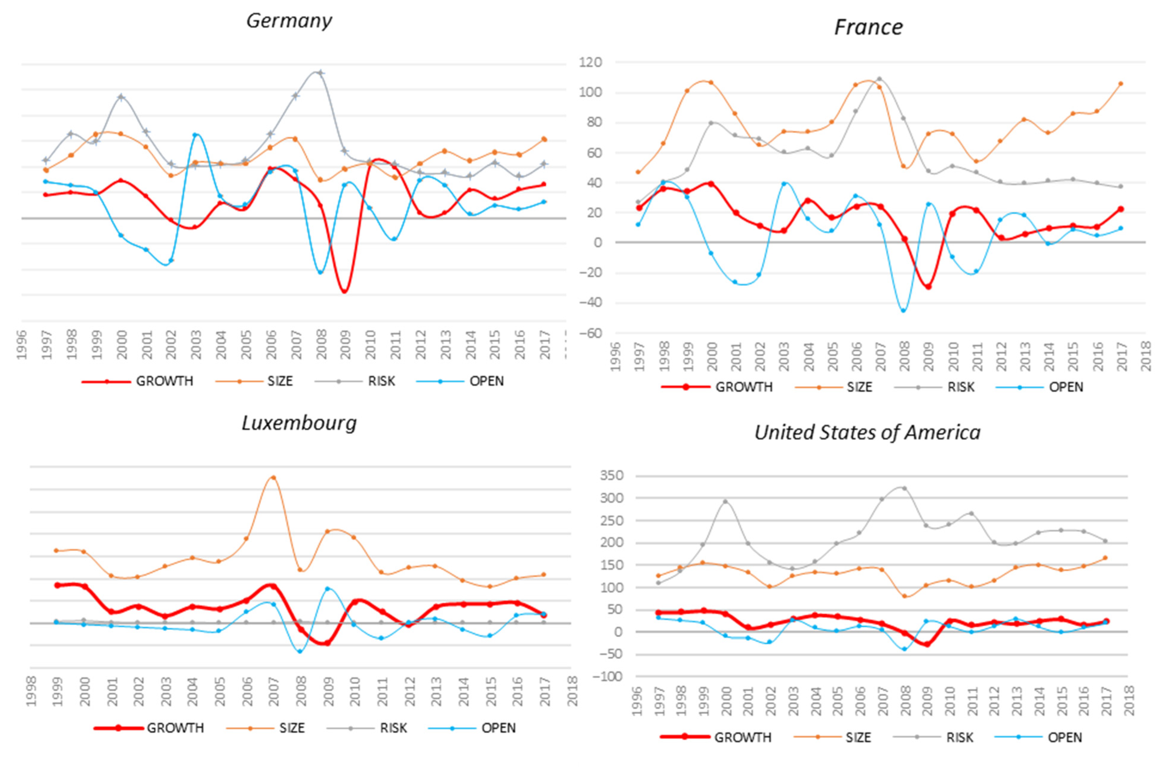
In order to highlight the data used in the regression, individual graphs are going to be presented in the following paragraph. Graphs include annual changes, expressed in percentage, of size, risk diversification, and openness of the national stock market and economic growth for Germany, France, Luxembourg, and the United States of America.
In Figure 1, a similar pattern can be seen among economic growth and stock market openness in all countries during the analysed period. Furthermore, the size of the stock market and economic growth presents a similar pattern, except that the drops had a stronger effect on economic growth than the increase in the trend. More interesting is that all four graphs present a one-year lag of the annual changes between the openness of the stock market and economic growth. The positive relationship between stock market openness and economic growth and stock market size and economic growth is clearly visible in the graphs below.
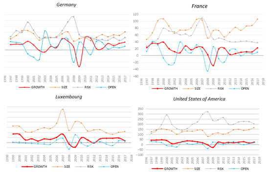
Figure 1.
Evolution of economic growth and size, risk diversification, and openness of the stock market in Germany, France, Luxembourg, and the USA.
From Figure 2, a positive relationship can be seen among openness of the stock market, marked with a yellow line and economic growth, marked with grey circles. A pattern can be seen where a higher openness level is associated with a higher position of the points representing the economic growth values. The same interpretation is feasible for the relationship between size and economic growth. It can be seen that an uprise in size determine higher positions of the economic growth points. Very low growth points are highly associated with lower values of all of the three parameters involved in the regression, specifically risk diversification, the level of stock market openness and the size of the stock market.
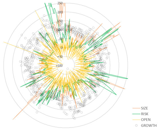
Figure 2.
Size, risk diversification, openness of the stock market and economic growth.
2.4.2. Testing for Stationarity, Cointegration and Multicollinearity
In order to avoid the biased results generated from the likely existence of unit roots in our variables, we tested for stationarity using the Augmented Dickey-Fuller Unit Root Test. The null hypothesis is that there is a unit root for the series. The alternative hypothesis being tested is that there is no unit root for the series and the series is stationary. We found the results presented in Table 2.

Table 2.
Stationarity test, authors source.
Results presented in Table 2 show that the computed p-value is lower than the significance level α (0.05), thus we reject the null hypothesis and accept the alternative hypothesis that there is no unit root for the series and the series is stationary. Next, we tested the series for long-run equilibrium between all variables by using the cointegration test of Johansen–Juselius procedure, the results being shown in Table 3.

Table 3.
Lambda max test, Johansen-Juselius procedure, authors source.
Both lambda and trace tests, from Table 3 and Table 4, indicate that the series is integrated with no differencing. Thus, we maintain that any shock to the system performed in the short run would quickly adjust to the equilibrium, in the long run, allowing the performance of an OLS (ordinary least squares) estimation only on the long-run model. The cointegration procedure shows the long-run relationship between size, volatility, liquidity, risk diversification and openness of the stock market. We also conducted the multicollinearity test to see if there is present non-randomness in data.

Table 4.
Trace test, Johansen-Juselius procedure, authors source.
The model passes the test for multicollinearity, as shown in Table 5, with the care for risk diversification-volatility and risk diversification-openness multicollinearity. Still, the value just surpasses the limit value of 3, being considered at the boundary of acceptance. As a consequence, it can be seen that the variables are moderately correlated, thus the multiple linear regression can be performed.

Table 5.
Multicollinearity test results, authors source.
2.4.3. Discussion and Analysis of Regression Results
In order to perform the estimation for economic growth, based on stock market indicators (liquidity, risk diversification, openness, volatility and size) we used ordinary least squares in a multiple linear regression, with control for human capital, financial market depth and investments, that led to the results shown in Table 6.

Table 6.
Results of the multiple linear regression.
One could see from Table 6 that liquidity has a nonsignificant influence over growth, in the present model, as same as volatility, considering that the p-values exceeded the α considered. Using our time series data, we found significant relationships among risk diversification and economic growth, the size of the stock market and economic growth, the level of openness and economic growth, supporting the results from [7,13,25,26,27]. Specifically, we found a 0.007% decrease (±0.004) in economic growth for every 1% increase in risk diversification, a 0.007% increase (±0.003) in economic growth for every 1% increase in the size of the stock market, and a 0.006% increase (±0.003) in economic growth for every 1% increase in the level of openness of the stock market. All results are reported to the national levels of the parameters and variables. It can be seen that risk diversification of the stock market and the size of the stock market in a country are the most significant factors when concerning the impact of the stock market on economic growth, in terms of GDP. Furthermore, volatility and liquidity do not transfer a significant impact on economic growth.
When considering the control variables, only human capital (education) and investments stabilized the model, with the remark that both had a significance level that exceeded the alfa considered. When running the regression weights, investments had a significant positive influence over volatility (8.72) and a negative relationship with the size of the stock market (−5.874). Human capital had a significant positive influence over liquidity and volatility (0.53 and 0.121). DEPTH parameter had a negative impact on risk diversification (−31.714) and openness of the stock market (−20.102).
Thus, the regression equation, after computing the regression would become:
For Equation (2), the multiple correlation coefficient is presented in Table 7.

Table 7.
Fitness of the multiple variable regression.
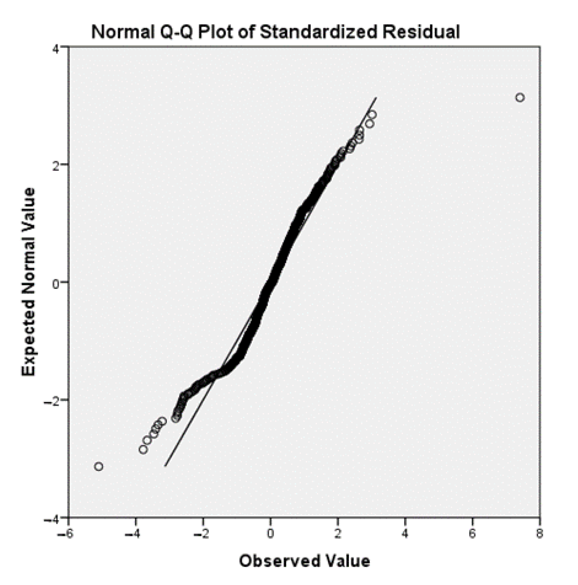
We also ran a Q-Q plot to present the good fit of our regression model, presented in Figure 3. It can be seen that the residuals have a normal distribution, thus the regression has a good fit.
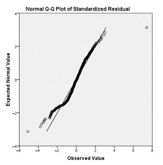
Figure 3.
Q-Q plot of standardized residuals.
In Figure 4, a three-dimensional hypercube is presented, involving all of the four parameters considered in the regression ran in the present paper (growth being the X axis, openness being the Y axis, size the Z axis, risk diversification being captured using a size scale on the upper-right edge of the cube). For the risk diversification, the thicker circle represents a higher value on the scale, while the thinner one represents a lower value on the scale.
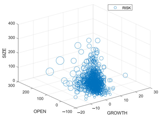
Figure 4.
Economic growth, openness, size and risk diversification of the stock market.
From Figure 4, one can draw some visible patterns of the growth-dependent parameter, in correlation with size and openness, while the regression results show a nonsignificant relationship among liquidity and growth and a negative relationship between risk diversification and economic growth. A higher level of economic growth can be associated with higher values of the size of the stock market. Furthermore, the regression results show a strong positive correlation between stock market openness and economic growth. When counting for risk diversification, a negative visible pattern can be drawn, where high levels of risk diversification are visible in the lower areas of economic growth.
3. Qualitative Approach
3.1. Introduction of Methodology (Sustainable Vector Model)
The heuristic methodologies of scientists have always been based on a quantitative perception, which hardly represents a qualitative approach of direct intuition of structural laws, which, thus, escaped the direct estimation. These representations led to the existence of a universe of fractal nature that is constituted on several levels of complexity of the information of the basic structures. The growth environment of the universe is considered to be such a fractal nature, fractal varieties being particular cases through which the support space is manifested.
The current economy is based on market principles that respond exclusively to human needs without taking into account ecosystem needs, therefore producing imbalances. Thus, it is necessary to model the principles of operation of this type of economy, in the fractalized model, which allows the development of the sustainability model in which all the accumulations produced are consumed by the internal cycles generated without exhausting external resources.
The transition from economic vectors to new or classic economic circuits would allow the transition with less risk to a model of a sustainable economy. The purpose of the fractalized model is to obtain a conceptual model of the sustainability of a complex system. As an early stage, the use of the model focuses on identifying feedback cycles and then switching diagrams. Then the model is structured on successive levels of determination, which are constructed by repeating, in different sizes, its structures in new and stable structures, that determines themselves. Thus, in the primary structure that converges to fractal modeling, a feedback structure is interposed in the form of a loop composed of three objects, namely the source, sensor and decision-maker together with the possibility of a portfolio of relationships between these three parameters.
3.2. Model Analysis
The qualitative approach is based on a sustainable vector model, that uses a group of automorphisms and a trivalent logic to construct a complex structure. The model is based on a group of automorphisms, composed of six functions, as follows: f1 = x; f2 = 1 − x; f3 = 1/x; f4 = 1 − 1/x; f5 = 1/(1 − x) and f6 = x/(x − 1) [32].
Automorphisms are used to create three new feedback waveform structures and the semantic significance of the functions introduced in the automorphism groups proposed, as follows: (a) f1 (x) = x defines the statement of existence (e.g., who); (b) f2 (x) = 1 − x defines the complementary symmetry on finite space (e.g., how); (c) f3 (x) = 1/x defines the inversion of the unit (e.g., what); (d) f4 (x) = 1 − 1/x defines the symmetry complementary to the inverse of the unit (e.g., where); (e) f5 (x) = 1/(1 − x) defines the inverse of the complementary symmetry on finite space (e.g., when); (f) f6 (x) = x/(1 − x) defines the relation of existence to complementary symmetry on finite space (e.g., why) [33].
Thus, we will approach the feedback structures, as in [34]. In Colceag’s hexavalent modeling, there will be two sets of generators: f1, f2, f3 and g1, g2, g3, so that f1*f2 = g3, f1*f3 = g2, f2*f3 = g1 and g1*g2 = f3, g1*g3 = f2, g2*g3 = f1. Colceag proposes, in his works, eight feedback structures, two of which represent cycles, (7) and (8), and another six commutative diagrams, (1)–(6), as represented in Figure 5.

Figure 5.
Structures in the sustainable vector model. Reproduced with permission from Colceag F.
The above triads were first proposed in [35], where triads are composed based on human interrelationships, thus the vectors used in the eight triads are assumed to connect persons in different levels. Feedback cycles and commutative diagrams are also presented in [36,37,38,39] where commutative diagrams are presented as transitive triads, while feedback cycles are to be mentioned as intransitive triads. In ref. [40] it is stated that a structure that is present in a network is a result of certain rules that maintain self-organization dynamics. In ref. [41] it is stated that these rules can cover institutional, cultural or social identity norms.
Using the figures above, different processes could be computed. Thus, the automorphism structures obtained allow the construction of both the six feedback cycles that are presented in the table and the construction of new feedback cycles obtained from new combinations of functions used. The concept of self-inhibiting or self-stimulating parameter is taken from Prigogine’s dissipative systems [42]. The new feedback cycles interconnect with the hexagonal structures identified in the fractal-type lattice automaton, which thus becomes a modeling system [43]. Some of these new feedback cycles that occur between hexagonal structures are presented in the next paragraphs. Figure 6 shows the basis for performing these new feedback cycles.
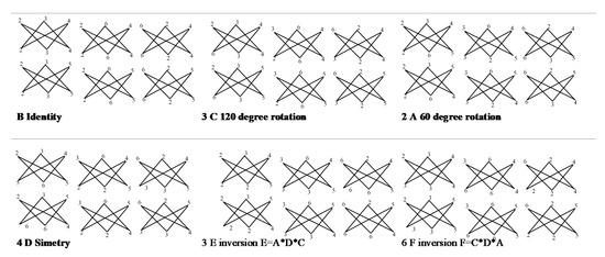
Figure 6.
Feedback structures in the sustainable vector model. Reproduced with permission from Colceag F.
The model itself is supposed to be evolutionary by moving from one level of complexity to another level of action complexity that generates new rules for stabilizing the processes that are involved. Thus, the construction of the model is a fractal [32], being obtained using octographic projection to transpose the hypercube of the group of automorphisms into a hexagonal shape. Fractals have the same structure on different levels, as illustrated in the successive enlargement of the Mandelbrot set [44,45,46]. Furthermore, being a fractal, it respects the Hausdorff—Besicovitch dimension [46], that is, calculated in Equation (3). The “fractal size” of the fractal usually “exceeds the topological size of the fractal” [47].
Furthermore, fractal models are characterized by fractal dimensions, but despite the fact that numbers measure complexity, these structures do not describe the uniqueness or specificity of details or the particular construction of fractal models [48]. The fractal model of hexagonal logic involves the introduction, based on a commutative diagram and feedback cycles, of a six-point formation that identifies with a hexagon. In the fractalization of this hexagon, hexagonal structures will appear on a smaller and smaller scale so that different levels of granulation and fractalization will be formed [49].
The construction of the model is based on the trivalent logic of Prigogine [50,51], as there has to exist: (a) a source (S), which is generating variation; (b) a sensor (&), which is able to know the essence of the variation; and (c) a decident (D), which is able to decide the subsequent behavior of the source, thus being able to decrease the level of variation (self-inhibition) or increase the amplitude of variation (self-simulation cycle) [52].
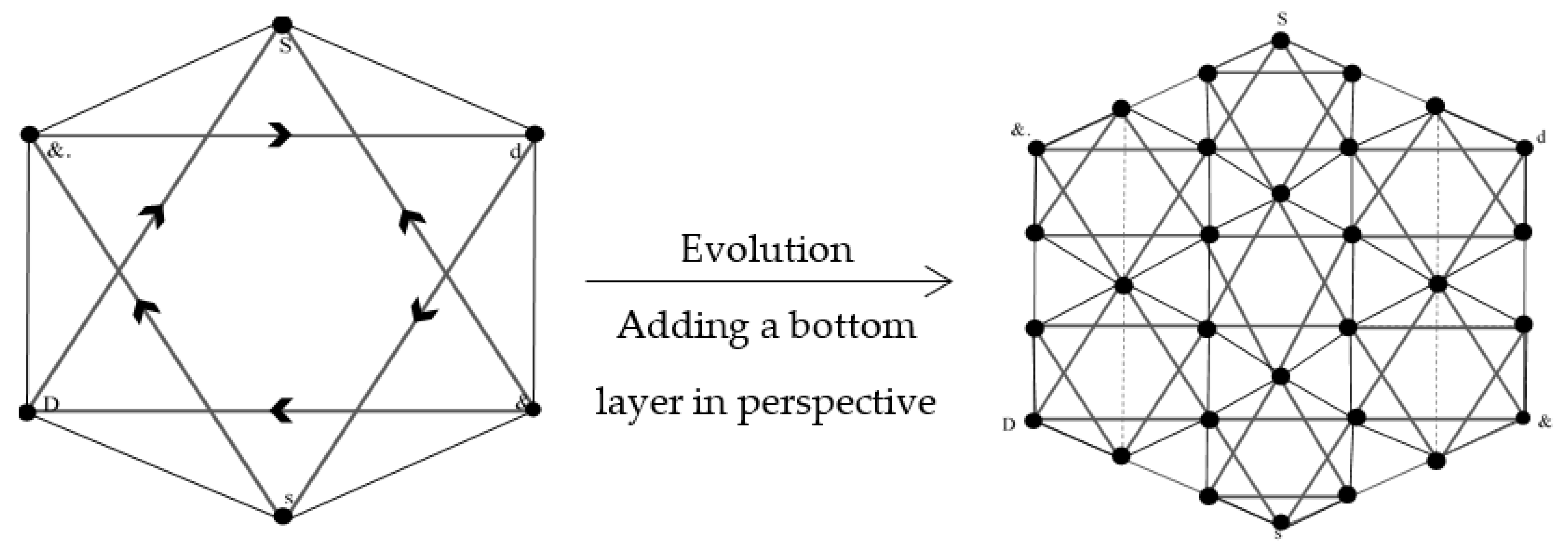
The switching diagram and the feedback cycle will be composed as follows. The model can be fractalized in many subdimensions. For example, in Figure 7, the third granulation level of the mode is presented. In essence, a system is divided into subsystems, which are modeled and can be divided in turn. From a three-dimensional point of view, the structure in the hypercubic space is divided into smaller structures.

Figure 7.
The structure of the model, containing: (a) a source (S), which is generating variation; (b) a sensor (&), which is able to know the essence of the variation; and (c) a decident (D), which is able to decide the subsequent behavior of the source, author’s source.
The granulation level represents the level up to which the subdivision of the basic hexagonal model reaches the fractalized structure. In the case of Figure 7, the granulation level is 2.
O the hexagonal structure computed, semantic order rules are applied, derived by the feedback structures presented in Figure 6. In Figure 8, we present the semantic order of the vectors that are being formed among points on the hexagonal form [33].

Figure 8.
Semantical order of vectors in the fractalized model, containing: a source (S), a sensor (&), and a decident (D), authors source.
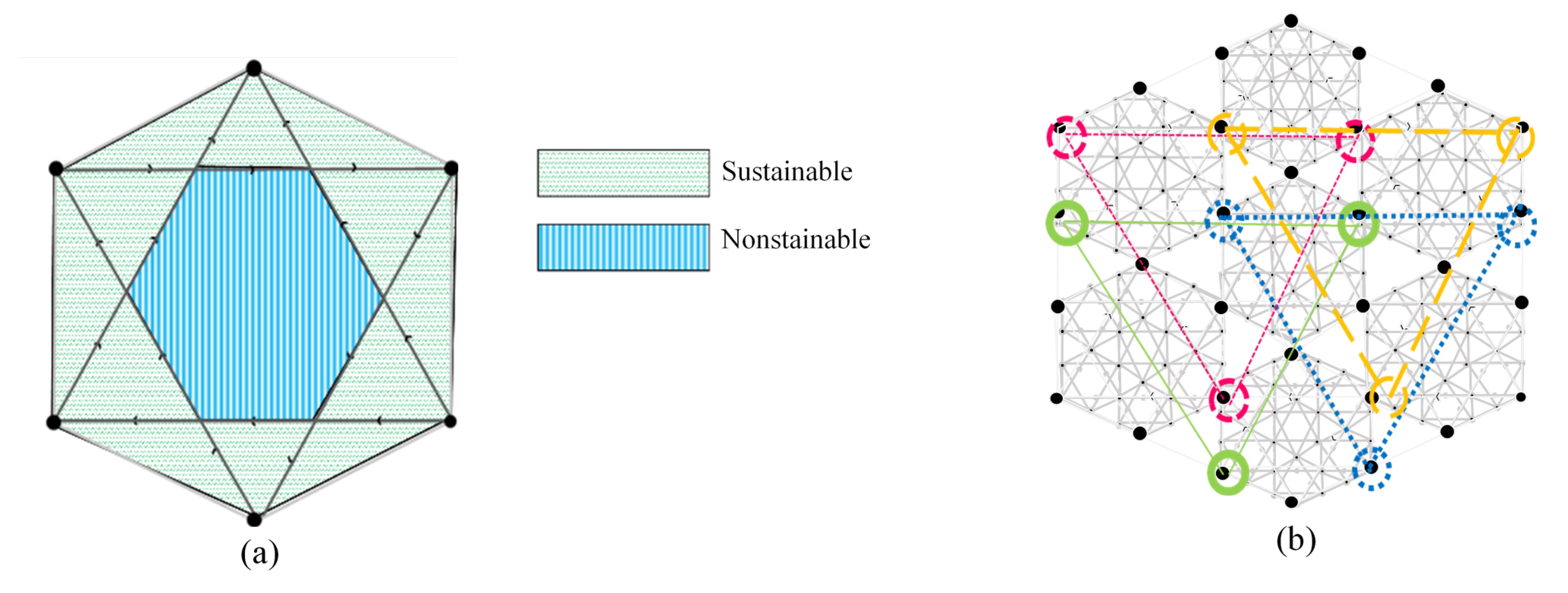
The level of fractalization refers to the sustainability and unsustainability of the component parts between a hexagonal structure, as presented in Figure 9a. Thus, the hexagonal structure that rests on the top is always sustainable, having the same behavior over time, and the hexagon that rests on the base is unsustainable and has the ability to produce changes. Additionally, in the presented model, interconnectivity of different points belonging to distinct dimensional substructures of fractal finite automata is generated by the octographic projection of the hypercube, as follows from Figure 9b.

Figure 9.
Fractalization (a) and interrelationships (b) in the model, as a result of the transposal of the hypercube, authors source.
The hexagonal figure is constructed on the basis of hexavalent logic, starting from the trivalent logic expounded by [49,52], where it is necessary to double the truth values of the trivalent logic creating a structure of six values that they derive from each other and define the modeling of a phenomenon in a certain context.
3.3. Results
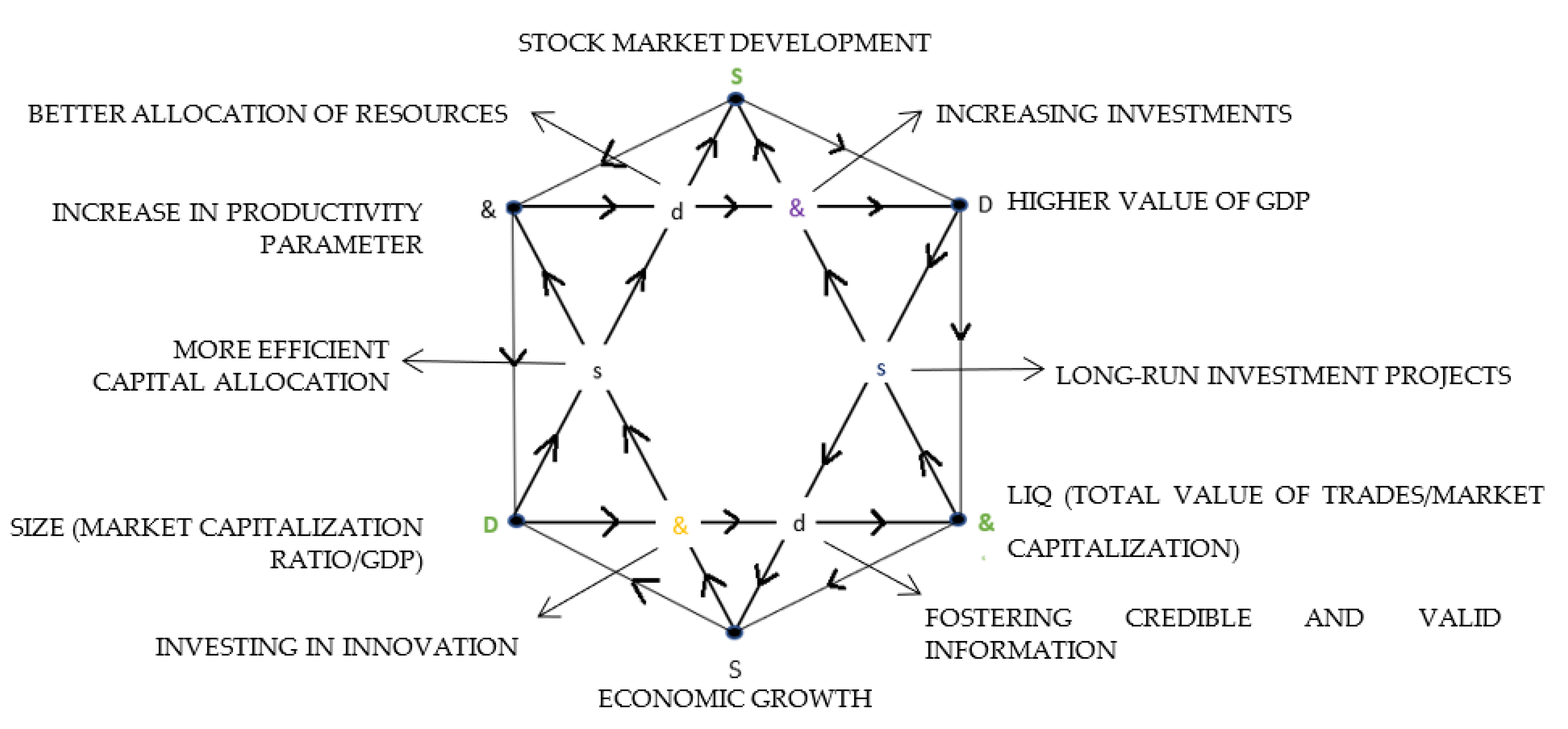
In Figure 10, the sustainable vector model applied in the context of economic growth is presented, using the stock market as an economic lever, thus being the phenomenon.
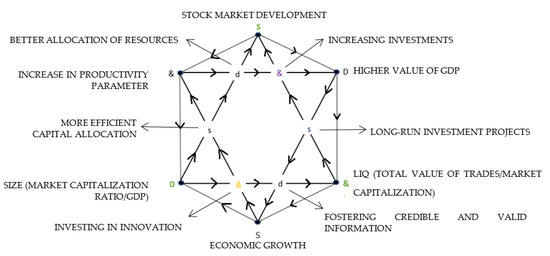
Figure 10.
Using the stock market as a lever to foster economic growth, containing: a source (S), a sensor (&), and a decident (D), authors source.
The model is constructed, as presented in the methodology, by using a group of automorphisms, composed of six functions, that can generate two feedback cycles and six commutative diagrams. Using the possible combination of vectors, we constructed a basic structure that integrates one big commutative diagram (the triangle with the tip upward), that has the accumulation point on the source and one big feedback cycle. The phenomenon triangle generates the two bottom-down vectors (between liquidity, economic growth and size), generating a feedback triangle between them. Vectors in the big feedback cycle triangle, with the tip downwards, will follow the direction computed on the vector between size and liquidity. From the source of the entire process (stock market development point), we can draw vectors on the outer edges of the hexagon, following a generating direction, considering that the source is nurturing the entire process.
This triangle represents the phenomena and integrated a source, a sensor and a decident. Because the phenomenon used is the stock market, the source of the triangle must be named “Stock market development”. In this upward triangle, the sensor (the level of sensibility) of the phenomenon is considered the liquidity of the stock market, in consideration that the liquidity of the stock market has a direct impact over the size of the stock market [12,13,14]. Thus, the decident is exactly the size of the stock market, with its variability having an intrinsic connection to the stock market development. If we seek to pursue the vectors in the phenomena triangle, both the stock market liquidity and size are generators for the development of the stock market. Therefore, as the rules of this trivalent logic conceive, every two points are able to generate the other.
The triangle representing the context has its source in the bottom down point of the representation, constructed as economic growth, considering that stock market development must have an impact on economic growth. In the context triangle, the sensitive parameter will be “Increase in productivity parameter”, considering the endogenous type of economic growth functions [53,54,55,56]. The own manifestation of the phenomenon is given by a higher value of GDP, this being the decident in the trivalent logic. Any two points on this triangle have the capacity to generate the third, as follows. A higher value of GDP and economic growth can generate increases in the productivity parameter [57,58,59,60,61], increases in productivity parameter and a higher value of GDP can generate economic growth [57,58,59,60,61], and increases in productivity parameter and economic growth generate a higher value of GDP.
As we could see, stock market development could be measured by the rate of liquidity as the total value of trades/market capitalization, and decided by its size measured as market capitalization ratio/GDP. In this context, economic growth is sensitive to the increase in the productivity parameter “A”, being decided by a higher value of the GDP.
3.4. Discussion of Model Analysis
In the smaller triangles, applying the trivalent logic of Prigogine, stock market development is sensitive to increasing investments, the decident being a higher value of GDP. It is also sensitive to the increase in productivity parameter, being decided by a better allocation of resources.
On the other hand, economic growth is sensitive to investments in innovation, being decided by size (market capitalization ratio/GDP) in this perspective. It is also sensitive to LIQ (total value of trades/market capitalization), being decided by credible and valid information.
In the right smaller triangle, long-run investment projects are sensitive to LIQ (total value of trades/market capitalization), the decident being a higher value of GDP.
In the left smaller triangle, more efficient capital allocation is sensitive to the increase in productivity parameter, being decided by size (market capitalization ratio/GDP).
Following the semantical order of the vectors, presented in Figure 8, one can outcome the relationships that are formed among different points of the process. Among the two sources on the structure, a causal relationship of having is presented, meaning that one’s existence will promote the other’s one growth, specifically the existence of economic growth will promote growth in the level of stock market development and vice versa.
When looking at the intrinsic connection of the existing relationship, among sensors on the big hexagonal form (increases in productivity parameter and liquidity of the stock market), the semantic rules imply that one cannot be without the other, meaning that the existence of liquidity in the stock market implies the existence if increases in productivity parameter and vice versa.
The causal relationship of doing, constructed on the semantic rules, among the decident on the big hexagon, implies that a higher value of GDP is performed by modifications in the size of the stock market (referred here as growth in the size of the stock market) and vice versa.
In the small hexagonal form, among the two sources, a causal relationship of protection is constructed, meaning that long-run investments projects must be protected by a more efficient capital allocation and vice versa. The relationship among the sensors, implying the act of creation, infers the fact by which increasing investments are creating investments in innovation and investments in innovation are creating an increasing investing process. Furthermore, between the decidents on the small hexagon, a “become” connection is created, conceiving that a better allocation of resources would become (or would be transposed) a process of fostering credible and valid information and vice versa.
The sustainable part of the process implies stock market development, LIQ (total value of trades/market capitalization), increase in productivity parameter, economic growth, size (market capitalization ratio/GDP) and higher value of GDP, allowing the whole structure to gain its own coherence, relevance and utility. The nonsustainable, nurturing process is structured on increasing investments, more efficient capital allocation, investing in innovation, better allocation of resources, fostering credible and valid information and long-run investment projects, the nonsustainable hexagon with its own dynamics and being defined by a high degree of instability.
4. Summary
It can be seen from the quantitative analysis that, among variables, there is a long-run equilibrium, after applying the Johansen–Juselius procedure. Additionally, the model passes the test for multicollinearity, with the care for risk diversification-volatility and risk diversification-openness multicollinearity. One could see from Table 6 that liquidity has a nonsignificant influence over growth, in the present model, the same as volatility. Openness and size of the stock market have a significant positive influence over economic growth, while risk diversification of the stock market presents a negative significant influence over economic growth, supporting the results from [7,13,27]. In opposition, the present findings contradict the results presented in [25,26], constraining a negative relationship between risk sharing and economic growth. In addition, contradicting present findings, [62] shows that “little evidence was found from the variance decomposition analysis that financial development “leads” economic growth”.
From the qualitative approach, we could conclude that the stock market could foster growth in a very complex way, constructed on a network of economic levers and systems. The process is bi-directional and is structured on a multivalent logic, being capable of a more complex structural transformation.
From the qualitative approach, the following conclusions could be drawn: the elements are grouped in three-field conglomerations; conglomerations have the capacity of circular permutation of three letters each; and the three basic elements are composed based on the automorphisms discussed in the present paper [32,33].
The qualitative model is also sustainable, competed by a series of factors. The relationship within the hexagonal fractalization system is performed through feedback loops and commutative diagrams, which allows self-stimulation and self-inhibition of the system as well as the formation of accumulation zones, while endogenous growth models develop their relationship through determination functions.
Within the fractalized system, complex relationships are formed, such as those of inter-relationship between different systems (initially formed in a hypercubic dimension). This allows the effects of changes in one parameter to be observed, even if the effects occur in another system. The automation group is sustainable because it is maintained and self-induced in the cascade, sustaining itself indefinitely. A sustainable and unsustainable structure is a relational structure, and it generates economic growth in a qualitative way, in the process of constructing the model.
The externalities of the hexagonal system will always determine new actions or processes, due to the feedback cycles in which they are involved. The externalities of endogenous models will have effects on other parameters only if they are introduced as determinants in the equations of those parameters.
Both types of models allow the addition of parameters for continuous endogenization. Thus, in the fractalized model, a new level of granulation can be added, and in the endogenous model, new functions for defining the included parameters can be added. The fractalized model is evolutionary in the sense that new levels of granulation can be created [32]. This is not an evolutionary model of growth, in the sense that it does not include Fircher’s replication equations [63], but it is an evolutionary modeling system, by developing new levels of granulation. If the fractalized approach model is transposed into a cellular automaton, then it helps in decision making and can become a decision model.
Within the endogenous model discussed in this paper, a series of correlations are formed that allow bivalent relationships of the introduced parameters. In the fractalized model, these correlations can be exposed using feedback cycles that form inside or between hexagons on different levels of fractalization. The endogenous model is based on bivalent logic, where the variations of the output parameter can be increasing or decreasing. In the fractalized model, the logic used is trivalent, so that a parameter is identified by a source, a sensor and a decision-maker. Thus, the parameter expressed by the source, measured by the sensor and capitalized by the decision-maker, can have several valences depending on the size of the sensor.
The relationship within the hexagonal fractalization system is performed through feedback loops and commutative diagrams, allowing self-stimulation and self-inhibition of the system and the formation of accumulation areas, while the endogenous growth model develops its relationship through determination functions.
Both models allow the determination of empirical evidence and comparative statistics. While the endogenous economic growth model allows the empirical study of the causality, having a probabilistic approach, the fractalized model allows the determination of a causal network, thus enhancing multiple future scenarios, also being a stochastic model.
Within the endogenous economic growth system, the modeling is quantitative, the units of measurement are quantitative, while the fractalized model assumes a qualitative measurement, by using syntactic operations. Automorphisms are interpreted as syntactic operations. This allows the correlation of the parameters with the help of qualitative mathematics.
Within the fractalized system, complex relationships are formed, such as those of interrelationships between different systems (initially formed in a hypercubic dimension). This allows the effects of changes in one parameter to be observed, even if the effects occur in another system.
The main control functions that the stock exchange has over the macroeconomic context, specifically over economic growth, are related to the regression results, which the present paper included. Thus, both liquidity and volatility of the stock market do not affect economic growth significantly, although other studies have found significant relationships, like in [22], where an increase in stock market liquidity may reduce savings due to lower uncertainty, thus slowing economic growth rate, or in [7], where increasing liquidity fosters growth in long term investment accessibility. Furthermore, in [21], excessive volatility in the stock market conducts to inefficiency in capital allocation, or lessens the credibility in investment operations, as in [30], thus reducing the rate of economic growth. A significant, positive influence has been found between economic growth and openness or size of the stock market, supporting the conclusions from [13], where openness could enhance economic growth by fostering foreign investors to find local equity prices, reducing the cost of capital, increasing market liquidity, and fostering financial productivity, and from [29], where the main control functions by which openness could enhance economic growth are: decreasing the cost of acquiring information, concluding contracts and making transactions in the banking system. Of course, when talking about stock market openness, the financial deregulations that could produce crises and financial booms and boosts should be well kept under control [27]. Additionally, the present results support the findings from [7], where the size of the stock market is an important characteristic of stock market development, with the remark that the size of the stock market is more relevant to investments and capital accumulation in highly developed markets, where volatility is more stable than in emerging markets [23]. The regression results show that risk diversification of the stock market presents a negative significant influence over economic growth, in contrast with the findings from [25], where reducing risk diversification would reduce economic growth and welfare, or from [26], where risk diversification also enhances the allocation of resources and accelerates economic growth. When taking into consideration the effect of the control variables over the parameters involved, we can see that volatility is positively influenced by investments and human capital, while the size of the stock market is negatively impacted by investments and DEPTH. Additionally, stock market liquidity is positively impacted by the level of education of one’s country citizens. Furthermore, DEPTH negatively impacts the openness of the stock market.
5. Conclusions
From the quantitative approach, one can conclude that that liquidity has a nonsignificant influence over growth, in the present model, the same as volatility, although high liquidity on the stock market “allows savers to buy and sell quickly and cheaply when they wish to alter their portfolios” [21]. By increasing liquidity in the stock market, long-term investments become more accessible [7]. In theory, volatility has an indirect relationship with economic growth, as excessive volatility in stock markets is conducive to inefficiency in capital allocation thus reducing the rate of economic growth. Furthermore, in [30], stock market volatility is observed due to a loss of credibility in investment operations. Openness and size of the stock market have a significant positive influence over economic growth, while risk diversification of the stock market presents a negative significant influence over economic growth. It can be seen from the quantitative analysis that, among variables, there is a long-run equilibrium between stock market development and economic growth, after applying the Johansen–Juselius procedure. Additionally, the model passes the test for multicollinearity, with the care for risk diversification-volatility and risk diversification-openness multicollinearity.
From the qualitative approach, we could conclude that the stock market could foster growth in a very complex way, constructed on a network of economic levers and systems. The process is bi-directional and is structured on a multivalent logic, being capable of a more complex structural transformation.
Both types of models allow the addition of parameters for continuous endogenization. Thus, in the fractalized model, a new level of granulation can be added, and in the endogenous model, new functions for defining the included parameters can be added.
The externalities of the hexagonal system will always determine new actions or processes, due to the feedback cycles in which they are involved. The externalities of endogenous models will have effects on other parameters only if they are introduced as determinants in the equations of those parameters.
Author Contributions
Conceptualization, R.-A.N. and M.F.; methodology, R.-A.N.; software, R.-A.N.; validation, R.-A.N., M.-P.C., M.F., F.S. and F.L.S.; formal analysis, R.-A.N.; investigation, R.-A.N.; resources, M.-P.C.; data curation, R.-A.N., M.F., F.S. and F.L.S.; writing—original draft preparation, R.-A.N.; writing—review and editing, R.-A.N.; visualization, R.-A.N.; supervision, M.-P.C. and F.S.; project administration, M.-P.C., F.S. and F.L.S.; funding acquisition, M.-P.C. All authors have read and agreed to the published version of the manuscript.
Funding
Project financed by Lucian Blaga University of Sibiu & Hasso Plattner Foundation research grants LBUS-IRG-2020-06.
Data Availability Statement
Data used for the liquidity, size and risk diversification of the stock market can be achieved at https://knoema.com/atlas/sources/WFE (accessed on 23 August 2021) (turnover ratio, market capitalization ratio and stock market total value trading ratio). The Standard & Poor’s/IFCI Global Composite Index is available at https://data.worldbank.org/indicator/CM.MKT.INDX.ZG (accessed on 23 August 2021). Stock price annual indexes can be found at https://data.oecd.org/price/share-prices.htm (accessed on 23 August 2021). Data regarding human capital can be achieved at https://data.oecd.org/education.htm (accessed on 23 August 2021). IMF Financial development index Database can be found at https://data.imf.org/?sk=F8032E80-B36C-43B1-AC26-493C5B1CD33B (accessed on 23 August 2021). Investments and GDP growth can be achieved at https://datatopics.worldbank.org/world-development-indicators/themes/economy.html (accessed on 23 August 2021).
Conflicts of Interest
The authors declare no conflict of interest.
References
- Kurz, H.D. On the growth of knowledge about the role of knowledge in economic growth: A critical assessment of recent literature on growth theory. In Innovation, Knowledge and Growth: Adam Smith, Schumpeter and the Moderns; Kurz, H.D., Ed.; Routledge: Abingdon-on-Thames, UK, 2013; pp. 87–115. [Google Scholar]
- Demirguc-Kunt, A.; Levine, R. Finance and Inequality: Theory and Evidence. Nber Work. Pap. 2009, in press. [Google Scholar]
- Pagano, M. Financial Markets and Growth: An Overview. Eur. Econ. Rev. 1993, 37, 613–622. [Google Scholar] [CrossRef]
- Caporale, G.M.; Howells, P.; Soliman, A.M. Endogenous Growth Models and Stock Market Development: Evidence from Four Countries. Rev. Dev. Econ. 2005, 9, 166–176. [Google Scholar] [CrossRef]
- Arrow, K.J. The Economic Implications of Learning by Doing. Rev. Econ. Stud. 1962, 29, 155. [Google Scholar] [CrossRef]
- Hughes, D.; Leethongdee, S.; Osiri, S. Social Science & Medicine Using Economic Levers to Change Behaviour: The Case of Thailand’ s Universal Coverage Health Care Reforms. Soc. Sci. Med. 2010, 70, 447–454. [Google Scholar] [CrossRef]
- Levine, R.; Zervos, S. Stock Market Development and Long-Run Growth. World Bank Econ. Rev. 1996, 10, 323–339. [Google Scholar] [CrossRef] [Green Version]
- Holmström, B.; Tirole, J. Market Liquidity and Performance Monitoring. J. Polit. Econ. 1993, 101, 678–709. [Google Scholar] [CrossRef]
- Schumpeter, J.A. The Theory of Economic Development, 3rd ed.; Harvard University Press: Cambridge, UK, 1934. [Google Scholar]
- Zhu, A.; Ash, M.; Pollin, R. Political Economy Stock Market Liquidity and Economic Growth: A Critical Appraisal of the Levine/Zervos Model; University of Massachusetts-Amherst: Amherst, MA, USA, 2002; manuscript in preparation. [Google Scholar]
- Wait, C.; Ruzive, T. The Influence of Financial Market Development on Economic Growth in BRICS Countries; Nelson Mandela Metropolitan University: Port Elizabeth, South Africa, 2016; manuscript in preparation. [Google Scholar]
- Mohtadi, H.; Agarwal, S. Stock Market Development and Economic Growth: Evidence from Developing Countries; University of Wisconsin-Milwaukee: Milwaukee, WI, USA, 2001; manuscript in preparation. [Google Scholar]
- Biedny, C. Financial Development and Economic Growth: Does Stock Market Openness Matter? J. Int. Bus. Law 2012, 11, 225–238. [Google Scholar]
- Rezina, S.; Jahan, N.; Mustafi, M.A.A. Contribution of StockMarket towards Economic Growth: An Empirical Study on Bangladesh Economy. Eur. Sci. J. 2017, 13, 238. [Google Scholar] [CrossRef] [Green Version]
- Pan, L.; Mishra, V. Stock Market Development and Economic Growth: Empirical Evidence from China. Econ. Model. 2018, 68, 661–673. [Google Scholar] [CrossRef]
- Ezeibekwe, O.F. Stock Market Development and Economic Growth: Empirical Evidence from Nigeria. Award. Excell. Stud. Res. Creat. Act.-Doc. 2019, 4. in press. [Google Scholar]
- Hondroyiannis, G.; Lolos, S.; Papapetrou, E. Financial Markets and Economic Growth in Greece, 1986–1999. Int. Financ. Mark. Inst. Money 2005, 15, 173–188. [Google Scholar] [CrossRef] [Green Version]
- Vazakidis, A.; Adamopoulos, A. Stock Market Development and Economic Growth an Empirical Analysis. Am. J. Econ. Bus. Adm. 2012, 4, 135–143. [Google Scholar] [CrossRef]
- Cooray, A.V. The Financial Sector and Economic Growth. Econ. Rec. 2009, 85, 10–21. [Google Scholar] [CrossRef] [Green Version]
- Rehman, M.A.U.; Shah, G.S.M.; Cioca, L.; Artene, A.E. Accentuating the Impacts of Political News on the Stock Price, Working Capital and Performance: An Empirical Review of Emerging Economy. Rom. J. Econ. Forecast. 2021, 2, 55–73. [Google Scholar]
- Arestis, P.; Demetriades, P.O.; Luintel, K.B. Financial Development and Economic Growth: The Role of Stock Markets. J. Quant. Methods 2018, 2, 43–55. [Google Scholar] [CrossRef]
- Bencivenga, V.R.; Smith, B.D. Financial Intermediation and Endogenous Growth. Rev. Econ. Stud. 1991, 58, 195–209. [Google Scholar] [CrossRef]
- Demirgüç-Kunt, A.; Levine, R. Stock Markets, Corporate Finance, and Economic Growth: An Overview. World Bank Econ. Rev. 1996, 10, 223–239. [Google Scholar] [CrossRef]
- Saint-paul, G. Fiscal Policy in an Endogenous Growth Model. Quqrterly J. Econ. 1992, 107, 1243–1259. [Google Scholar] [CrossRef]
- Devereux, M.B.; Smith, G.W. International Risk Sharing and Economic Growth. Int. Econ. Rev. 1998, 32, 257–273. [Google Scholar] [CrossRef]
- Obstfeld, M. Risk-Taking, Global Diversification, and Growth. Am. Econ. Rev. 1994, 84, 1310–1329. [Google Scholar] [CrossRef]
- Korajczyk, R. A Measure of Stock Market Integration for Developed and Emerging Markets. World Bank Econ. Rev. 1996, 10, 267–289. [Google Scholar] [CrossRef] [Green Version]
- Schmukler, S.L.; Kaminsky, G.L. Short-Run Pain, Long-Run Gain: The Effects of Financial Liberalization. IMF Work. Pap. 2003, 3, 1. [Google Scholar] [CrossRef] [Green Version]
- Levine, R. International Financial Liberalization and Economic Growth. Rev. Int. Econ. 2001, 9, 688–702. [Google Scholar] [CrossRef]
- Peress, J. Learning from Stock Prices and Economic Growth. CEPR Discussion Paper No. DP8569. Available online: https://ssrn.com/abstract=1928452 (accessed on 20 August 2021).
- Patro, S.G.K.; Sahu, K.K. Normalization: A Preprocessing Stage; Gandhi Institute of Engineering and Technology: Gunupur, India, 2015; manuscript in preparation. [Google Scholar]
- Colceag, F. Cellular Automata; Algebraic Fractals. Available online: http://austega.com/florin/CellularAutomataAlgebraicFractals.htm (accessed on 1 September 2020).
- Colceag, F. Universul Evolutiv. Available online: https://sustainability-modeling.com/ (accessed on 1 September 2020).
- Caraiani, C.; Lungu, C.I.; Dascălu, C.; Colceag, F. Green Accounting Initiatives and Strategies for Sustainable Development; IGI Global: Hershey, PA, USA, 2015; ISBN 9781466687219. [Google Scholar]
- Davis, J.A.; Leinhardt, S. The Structure of Positive Interpersonal Relations in Small Groups; National Opinion Research Center: Chicago, IL, USA, 1967. [Google Scholar]
- Johnsen, E.C. Network Macrostructure Models for the Davis-Leinhardt Set of Empirical Sociomatrices. Soc. Netw. 1985, 7, 203–224. [Google Scholar] [CrossRef]
- Moody, J. Matrix Methods for Calculating the Triad Census. Soc. Netw. 1998, 20, 291–299. [Google Scholar] [CrossRef]
- Lienert, J.; Koehly, L.; Reed-Tsochas, F.; Marcum, C.S. An Efficient Counting Method for the Colored Triad Census. Soc. Netw. 2019, 58, 136–142. [Google Scholar] [CrossRef] [Green Version]
- Holland, P.W.; Leinhardt, S. Structural Models of Small Groups. Comp. Gr. Stud. 1971, 2, 107–124. [Google Scholar] [CrossRef]
- Kogut, B. The Network as Knowledge: Generative Rules and the Emergence of Structure. Strateg. Manag. J. 2000, 21, 405–425. [Google Scholar] [CrossRef]
- Cugmas, M.; Ferligoj, A.; Ziberna, A. Generating Global Network Structures by Triad Types. PLoS ONE 2018, 13, 1–24. [Google Scholar] [CrossRef]
- Prigogine, I. From Being to Becoming: Time and Complexity in the Physical Sciences; W. H. Freeman And Company: New York, NY, USA, 1984; ISBN 0716711079. [Google Scholar]
- Colceag, F. Introduction in the Algebric Fractures, the Cosmic Perspective. Sustain. Model. 2018, 1–4. [Google Scholar] [CrossRef]
- Mandelbrot, B.B. Fractal Geometry of Nature, 2nd ed.; Times Books: New York, NY, USA, 2008; ISBN 9788578110796. [Google Scholar]
- Briggs, J. The Patterns of Chaos; Touchstone: New York, NY, USA, 1992. [Google Scholar]
- Kenneth, F. Fractal Geometry: Mathematical Tools for Physicists, 3rd ed.; John Wiley & Sons, Ltd.: Chichester, UK, 2006; ISBN 9783527405480. [Google Scholar]
- Mandelbrot, B. Fractals and Chaos; Springer: New York, NY, USA, 2004; ISBN 0387201580. [Google Scholar]
- Karperien, A.L. Defining Microglial Morphology; Form, Function, and Fractal Dimension. Master’s Thesis, Charles Sturt University, Wagga, Australia, 2014. [Google Scholar]
- Colceag, F. The Alphabet of the Art of Thinking. Available online: https://sustainability-modeling.com/ (accessed on 20 August 2020).
- Prigogine, I.; Nicolis, G. Self-Organisation in Nonequilibrium Systems: Towards a Dynamics of Complexity. Bifurc. Anal. 1985, 3, 3–12. [Google Scholar]
- Prigogine, I.; Stengers, I. Order out of Chaos: Man’s New Dialogue with Nature; Bantam New Age Books: New York, NY, USA, 1984; ISBN 0553340824. [Google Scholar]
- Colceag, F. Model Economic Vectorial Sustenabil. Available online: https://sustainability-modeling.com/ (accessed on 1 September 2020).
- Ugur, M. Modeling Growth: Exogenous, Endogenous and Schumpeterian Growth Models. Greenwich Pap. Polit. Econ. 2016, 37, 1–23. [Google Scholar]
- Sharipov, I. Contemporary Economic Growth Models and Theories: A Literature Review. CES Work. Pap. 2015, VII, 759–773. [Google Scholar]
- Alcouffe, A.; Kuhn, T. Schumpeterian Endogenous Growth Theory and Evolutionary Economics. J. Evol. Econ. 2004, 14, 223–236. [Google Scholar] [CrossRef]
- Aghion, P.; Howitt, P. A Model of Growth through Creative Destruction. Econometrica 1992, 60, 323. [Google Scholar] [CrossRef]
- Solow, R.M. A Contribution to the Theory of Economic Growth. Quartely J. Econ. 1956, 70, 65–94. [Google Scholar] [CrossRef]
- Swan, T. Economic Growth and Capital Accumulation. Econ. Rec. 1957, 33, 103–108. [Google Scholar] [CrossRef]
- Romer, P.M. Endogenous Technological Change. J. Polit. Econ. 1990, 98, S71–S102. [Google Scholar] [CrossRef] [Green Version]
- Lucas, R.E. On the Mechanics of Economic Development. J. Monet. Econ. 1988, 22, 3–42. [Google Scholar] [CrossRef]
- Guarini, G. Innovation and Growth in the Grossman-Helpman’s 1991 Model with Increasing Returns. Econ. Bull. 2011, 31, 147–155. [Google Scholar]
- Shan, J. Does Financial Development “lead” Economic Growth? A Vector Auto-Regression Appraisal. Appl. Econ. 2005, 37, 1353–1367. [Google Scholar] [CrossRef]
- Marx, K. Capital and Other Writings of Karl Marx; Eastman, M., Ed.; Carlton House: New York, NY, USA, 1923. [Google Scholar]
Publisher’s Note: MDPI stays neutral with regard to jurisdictional claims in published maps and institutional affiliations. |
© 2021 by the authors. Licensee MDPI, Basel, Switzerland. This article is an open access article distributed under the terms and conditions of the Creative Commons Attribution (CC BY) license (https://creativecommons.org/licenses/by/4.0/).

