Dynamical Analysis of Bio-Ethanol Production Model under Generalized Nonlocal Operator in Caputo Sense

Abstract

The nonlinear fractional-order model of bioethanol production under a generalized nonlocal operator in the Caputo sense is investigated in this work. Theoretical and computational aspects of the considered model are discussed. We prove that the model has at least one solution and a unique solution using the Leray–Schauder and Banach contraction theorems. Using functional analysis, we investigate several types of Ulam–Hyres model stability. We use the predictor–corrector (P–C) method to construct a broad numerical scheme for the model’s solution. The proposed numerical method’s stability is demonstrated. Finally, we depict the numerical findings geometrically to demonstrate the model’s dynamics.

1. Introduction and Motivation

Scientists and industry have been focusing on the creation of green, sustainable biorefineries in recent years. This concept implies the production of a wide range of molecules from sustainable sources such as biomass, fine chemicals, or energy [1,2]. Processes based on the conversion of biomass into useable biomaterial might increase the economic worth of currently discarded raw materials while also reducing wastewater released by various industries. Bioethanol is one of the most important renewable fuels, and it helps to reduce the negative environmental effects of global fossil fuel use. Ethanol can be added to gasoline as a transportation fuel to minimize the number of greenhouse gases released into the atmosphere [3]. One of the really efficient renewable liquid biofuels for replacing oil-derived fossil fuels is bioethanol. Agricultural crops are now the most common substrates for bioethanol synthesis (sorghum, corn, sugarcane, wheat). Determining the growth rate of biomass is critical to understanding how bioethanol production works in a bioreactor. There are various models that examine the dynamics of cell mass growth in a bioreactor, and the majority of these models offer formulations for the specific cell mass growth rate [3,4]. Several scientists were interested in looking at the long-term behavior of expanded models that included a continuous flow reactor [5,6]. In systems with pure and simple microbial competition, Ajbar investigated the conditions for the formation of complex dynamic behavior [7]. In 2013, Cornelli et al. investigated yeasts’ ability to ferment sugars found in a variety of items made by well-known companies [8]. In 2016, Cornelli et al. published an ethanol production model based on the performance of ten commercial Saccharomyces yeast strains in the batch alcoholic fermentation of sugars acquired from the soft drink industry [9]. In 2018, Bhowmik et al. [10] extended the process model of Cornelli et al. by including recycle ratio and decay rate. Their model contains three contents explaining the evolution of substrate $\mathcal{S}$, biomass $\mathcal{X}$ and ethanol $\mathcal{E}.$ They formulated a model for bioethanol productions as:

$$\left\{\begin{array}{c}\mathbb{V}\frac{d}{dt}\mathcal{S}=\mathrm{F}({\mathcal{S}}_0-\mathcal{S})-\frac{{\mu }_{max}}{{\mathrm{Y}}_{\frac{\mathcal{X}}{\mathcal{S}}}}{\mathbb{M}}_2(\mathcal{S},\mathcal{E})\mathcal{X}\mathbb{V},\hfill \\ \mathbb{V}\frac{d}{dt}\mathcal{X}=-\mathrm{F}\mathcal{X}+{\mu }_{max}{\mathbb{M}}_2(\mathcal{S},\mathcal{E})\mathcal{X}\mathbb{V}+\mathrm{R}\mathrm{F}(\mathrm{C}-1)\mathcal{X}-{\mathrm{b}}_{\mathrm{H}}\mathcal{X}\mathbb{V},\hfill \\ \mathbb{V}\frac{d}{dt}\mathcal{E}=-\mathrm{F}\mathcal{E}+{\mathrm{Y}}_{\frac{\mathcal{E}}{\mathcal{X}}}{\mu }_{max}{\mathbb{M}}_2(\mathcal{S},\mathcal{E})\mathcal{X}\mathbb{V}+\mathrm{R}\mathrm{F}(\mathrm{C}-1)\mathcal{E}+\mathrm{F}\gamma \mathcal{X},\hfill \end{array}\right.$$

where ${\mathbb{M}}_2$ represents the modified Andrew expression with inhibition by ethanol. ${\mathbb{M}}_2$ and residence time $\tau$ are respectively defined as:

$$\begin{array}{cc}\hfill {\mathbb{M}}_2(\mathcal{S},\mathcal{E})& =\frac{\mathcal{S}}{{\mathrm{K}}_{\mathcal{S}}+\mathcal{S}+{\mathrm{K}}_{\mathcal{E}}{\mathcal{E}}^2},\hfill \\ \hfill \tau & =\frac{\mathbb{V}}{\mathrm{F}}.\hfill \end{array}$$

The first equation of the above model represents the rate of change of the substrate. The rate of flow through the reactor and the biomass’ use of the substrate determine this rate. The first term of the equation indicates the change in $\mathcal{S}$ due to the flow through the reactor, while the last term represents the negative rate of change in $\mathcal{S}$ concentration owing to biomass consumption of the substrate.

The rate of change in biomass is represented by the model’s second equation. This rate is determined by the reactor flow, $\mathcal{S}$ consumption, and the presence of a settling unit. The change in $\mathcal{X}$ concentration caused by the flow-through reactor is given by the first term on the right-hand side of the second equation. The positive change in the concentration of $\mathcal{X}$, owing to the consumption of $\mathcal{S}$, is represented by the second term. The third term indicates settling unit consumption, while the fourth term depicts $\mathcal{X}$ elimination owing to a combination of first-order processes that include cell loss and cell breakdown.

The third equation of the model represents the rate of change of the ethanol. It depends on the use of a settling unit and a flow-through reactor. The first term of the third equation gives the change of concentration of ethanol due to flow via reactor. The second term represents the increase in the concentration of ethanol due to the use of $\mathcal{S}.$ The third term gives the use of a settling unit. The fourth term models the production of ethanol by maintenance.

Fractional calculus has recently been used to describe a variety of complex problems in the domains of computational sciences [11,12]. Because of the complexity of these issues, researchers have developed mathematical theories to simulate the complexities of nature using fractional calculus. Differential equations and differential operators are needed to develop mathematical models, which are effective tools for explaining real-world issues. The differential operators can be either local or nonlocal (fractional). The most well known fractional operators are of three types: operator with a power-law kernel is called Caputo operator [13], operator with exponential decay law is called Caputo–Fabrizio operator [14], and finally, operator with Mittag–Leffler law is called Atangana–Baleanu operator [15]. These operators are commonly employed by researchers to capture memory features of mathematical models, which may be found in a variety of fields of study [16,17,18]. As the use of fractional differential equations grows, researchers have begun to develop novel methods for numerically solving these equations, as they confront numerous challenges while solving these equations analytically. The methods which are available in literature include the predictor–corrector method (P–C) [19], the Adams–Bashforth scheme [20], the Adomain decomposition method [21], the fractional differential transform method [22], and the homotopy analysis method [23], and so forth. Different theoretical aspects of fractional differential equations are also studied by researchers in the last century. Existence theory, stability analysis, numerical and optimization approaches are some of the well-known features that have recently been introduced.

Many nonlocal operators are available in the literature, which have important applications in applied mathematics. In 2014, Katugampola introduced a new fractional derivative and integral which generalizes Riemann–Liouville and the Hadamard fractional derivative and integrals [24,25]. Recently, Odibat and his coauthor constructed a new generalized Caputo fractional derivative which generalizes the classical Caputo derivative [26]. There are various applications of generalized Caputo fractional derivative in the literature. For instance, Kumar et al. studied a love story model of Layla and Manjnun using a new GCF operator [27]. In the literature [28], the authors have analyzed the HIV model via the GCF derivative and many more. Predictor–corrector (P–C) algorithms, on the other hand, are one of the most efficient, reliable, and accurate methods for numerically solving FDEs, where the fractional derivative is regarded in the Caputo sense. The numerical solution of the initial value problem with the Caputo fractional differential equation has been introduced in [19] using an Adams-type P–C technique. In the literature, this approach has been widely utilized to simulate several fractional derivative models, including the work reported in [29,30,31,32].

Since the considered generalized fractional derivative is the generalization of classical Caputo derivative. This derivative has recently introduced and its applications in modelling of any physical phenomena are very rare. We use this newly developed generalized Caputo derivative to study the bioethanol model. We study the theoretical and computational aspects of the above ethanol production model. The major goal of this study is to look into the existence and uniqueness of the model’s solutions using well-known fixed point theorems like Banach’s and Larey-nonlinear Schauder’s alternative. Furthermore, the stability analysis is explored from the perspective of various Ulam’s stabilities. Finally, we apply the predictor–corrector approach to determine the fractional model of ethanol production’s approximate solutions. We proved the stability of the proposed numerical method in the last theorem of the paper. The numerical results are graphically presented to study the process of the ethanol production and effects of the generalized Caputo operator on the evolution of the proposed ethanol model.

2. Preliminaries

This section provides some fundamental concepts which are needed for our current study. For the sake of simplicity, we will use GFI for generalized fractional integral and GFD for generalized fractional derivative.

Definition 1

([25]). The GFI of a function $\mathrm{Y}$ of order ${\kappa }_2>0$ is expressed as ${}^{{\kappa }_1}{\mathcal{I}}_{a^{{}_{+}}}^{{\kappa }_2}$ and is defined as:

$$\left({}^{{\kappa }_1}{\mathcal{I}}_{b^{{}_{+}}}^{{\kappa }_2}\mathrm{Y}\right)(t)=\frac{1}{\Gamma ({\kappa }_2)}\left[{\int }_b^t{(\frac{t^{{\kappa }_1}-s^{{\kappa }_1}}{{\kappa }_1})}^{{\kappa }_2-1}\mathrm{Y}(s)\frac{ds}{s^{1-{\kappa }_1}}\right],t>b\ge 0,$$

where ${\kappa }_1>0.$

Definition 2

([24]). The GFD of a function $\mathrm{Y}$ of order ${\kappa }_2>0$ in RL sense is expressed as ${}_{RL}^{{\kappa }_1}{\mathbf{D}}_{b^{+}}^{{\kappa }_2}$ and is defined as:

$$\left({}_{RL}^{{\kappa }_1}{\mathbf{D}}_{b^{+}}^{{\kappa }_2}\mathrm{Y}\right)(t)=\frac{{(t^{1-{\kappa }_1}\frac{d}{dt})}^j}{\Gamma (j-{\kappa }_2)}{\int }_b^t{(\frac{t^{{\kappa }_1}-s^{{\kappa }_1}}{{\kappa }_1})}^{j-{\kappa }_2-1}\mathrm{Y}(s)\frac{ds}{s^{1-{\kappa }_1}},t>b\ge 0,$$

where ${\kappa }_1>0$ and $j\in \mathbb{N}$.

Definition 3

([26]). The new GFD of a function $\mathrm{Y}$ of order ${\kappa }_2>0$ in Caputo sense is expressed as ${}^{{\kappa }_1}{\mathbf{D}}_{b^{+}}^{{\kappa }_2}$ and is defined as:

$$\left({}^{{\kappa }_1}{\mathbf{D}}_{b^{+}}^{{\kappa }_2}\mathrm{Y}\right)(t)=\frac{1}{\Gamma (j-{\kappa }_2)}{\int }_b^t{(\frac{t^{{\kappa }_1}-s^{{\kappa }_1}}{{\kappa }_1})}^{j-{\kappa }_2-1}{(t^{1-{\kappa }_1}\frac{d}{dt}\mathrm{Y})}^j(s)\frac{ds}{s^{1-{\kappa }_2}},$$

where ${\kappa }_2\in (j-1,j].$

Lemma 1

([26]). Let $\mathrm{Y}\in {\mathfrak{C}}^j([b,c]),$ $j-1<{\kappa }_2\le j$ and ${\kappa }_1>0.$ Then, for $0\le b<t\le c<\infty$, we have

$$\left({}^{{\kappa }_1}{\mathcal{I}}_{b^{{}_{+}}}^{{\kappa }_2}{}^{{\kappa }_1}{\mathbf{D}}_{b^{+}}^{{\kappa }_2}\mathrm{Y}\right)(t)=\mathrm{Y}(t)-\sum _{g=0}^{j-1}\frac{{(t^{1-{\kappa }_1}\frac{d}{dt})}^g(\mathrm{Y})(b)}{\Gamma (g+1)}{(\frac{t^{{\kappa }_1}-s^{{\kappa }_1}}{{\kappa }_1})}^g.$$

(1)

If ${\kappa }_2\in (0,1],$ then

$$\left({}^{{\kappa }_1}{\mathcal{I}}_{b^{{}_{+}}}^{{\kappa }_2}{}^{{\kappa }_1}{\mathbf{D}}_{b^{+}}^{{\kappa }_2}\mathrm{Y}\right)(t)=\mathrm{Y}(t)-\mathrm{Y}(b).$$

Theorem 1

(Banach contraction result). Let $\mathcal{A}$ represents a Banach space, and $Ø\ne \mathbb{B}\subset \mathcal{A}$ be a closed subset. If the operator $\mathcal{F}:\mathbb{B}\to \mathbb{B}$ fulfills the contraction condition, the $\mathcal{F}$ has a unique fixed point in $\mathbb{B}$.

Theorem 2

(Leray–Schauder fixed point theorem). Let ${\mathbb{B}}_r$ be a convex and closed subset of $\mathcal{A}$. Let $0\in \mathbb{P},$ where $\mathbb{P}$ is an open subset of $\mathcal{A}.$ If $\mathcal{F}:\overline{\mathbb{P}}\to$ ${\mathbb{B}}_r$ is a compact and continuous map. Then either $\mathcal{F}$ possesses a fixed point in $\overline{\mathbb{P}}$ or $\exists \Theta \in \partial$$\overline{\mathbb{P}}$ and $\psi \in (0,1)$ such that $\Theta =\psi \mathcal{F}(\Theta )$.

3. Model Formulation and Its Analysis

Here, we formulate the above model given by using generalized Caputo fractional order operator. We formulate the fractional order dimensional model as:

$$\left\{\begin{array}{c}\mathbb{V}{}^{{\kappa }_1}{\mathbf{D}}^{{\kappa }_2}\mathcal{S}=\mathrm{F}({\mathcal{S}}_0-\mathcal{S})-\frac{{\mu }_{max}}{{\mathrm{Y}}_{\frac{\mathcal{X}}{\mathcal{S}}}}{\mathbb{M}}_2(\mathcal{S},\mathcal{E})\mathcal{X}\mathbb{V},\hfill \\ \mathbb{V}{}^{{\kappa }_1}{\mathbf{D}}^{{\kappa }_2}\mathcal{X}=-\mathrm{F}\mathcal{X}+{\mu }_{max}{\mathbb{M}}_2(\mathcal{S},\mathcal{E})\mathcal{X}\mathbb{V}+\mathrm{R}\mathrm{F}(\mathrm{C}-1)\mathcal{X}-{\mathrm{b}}_{\mathrm{H}}\mathcal{X}\mathbb{V},\hfill \\ \mathbb{V}{}^{{\kappa }_1}{\mathbf{D}}^{{\kappa }_2}\mathcal{E}=-\mathrm{F}\mathcal{E}+{\mathrm{Y}}_{\frac{\mathcal{E}}{\mathcal{X}}}{\mu }_{max}{\mathbb{M}}_2(\mathcal{S},\mathcal{E})\mathcal{X}\mathbb{V}+\mathrm{R}\mathrm{F}(\mathrm{C}-1)\mathcal{E}+\mathrm{F}\gamma \mathcal{X}.\hfill \end{array}\right.$$

(2)

The initial values of the three components of the considered model are all non-negative, that is, $\mathcal{S}(0)={\mathcal{S}}_0>0,\mathcal{X}(0)={\mathcal{X}}_0\ge 0,$ and $\mathcal{E}(0)={\mathcal{E}}_0\ge 0.$ Now, the model (2) can be reduced to dimensionless form by introducing the dimensionless variables as:

$${\mathcal{S}}^{*}=\frac{\mathcal{S}}{{\mathrm{K}}_{\mathcal{S}}},{\mathcal{X}}^{*}=\frac{\mathcal{X}}{{\mathrm{Y}}_{\frac{\mathcal{E}}{\mathcal{X}}}{\mathrm{K}}_{\mathcal{S}}},{\mathcal{E}}^{*}=\frac{\mathcal{E}}{{\mathrm{K}}_{\mathcal{S}}},t^{*}={\mu }_{max}t.$$

The dimensionless model is given as:

$$\left\{\begin{array}{c}{}^{{\kappa }_1}{\mathbf{D}}^{{\kappa }_2}{\mathcal{S}}^{*}(t^{*})=\frac{{\mathcal{S}}_0^{*}-{\mathcal{S}}^{*}}{{\tau }^{*}}-\frac{{\mathcal{S}}^{*}{\mathcal{X}}^{*}}{1+{\mathcal{S}}^{*}+{\gamma }_1{\mathcal{E}}^{{*}^2}},\hfill \\ {}^{{\kappa }_1}{\mathbf{D}}^{{\kappa }_2}{\mathcal{X}}^{*}(t^{*})=\frac{-{\mathcal{X}}^{*}}{{\tau }^{*}}+\frac{{\mathcal{S}}^{*}{\mathcal{X}}^{*}}{1+{\mathcal{S}}^{*}+{\gamma }_1{\mathcal{E}}^{{*}^2}}-{\mathrm{b}}_{\mathrm{H}}^{*}{\mathcal{X}}^{*}+\frac{{\mathrm{R}}^{*}{\mathcal{X}}^{*}}{{\tau }^{*}},\hfill \\ {}^{{\kappa }_1}{\mathbf{D}}^{{\kappa }_2}{\mathcal{E}}^{*}(t^{*})=\frac{-{\mathcal{E}}^{*}}{{\tau }^{*}}+\frac{{\gamma }_2{\mathcal{X}}^{*}}{{\tau }^{*}}+\frac{{\gamma }_3{\mathcal{S}}^{*}{\mathcal{X}}^{*}}{1+{\mathcal{S}}^{*}+{\gamma }_1{\mathcal{E}}^{{*}^2}}+\frac{{\mathrm{R}}^{*}{\mathcal{E}}^{*}}{{\tau }^{*}}.\hfill \end{array}\right.$$

(3)

The parameters of model (3) are non-negative and also the initial values are ${\mathcal{S}}^{*}(0)={\mathcal{S}}_0^{*}\ge 0$, ${\mathcal{X}}^{*}(0)={\mathcal{X}}_0^{*}\ge 0$, and ${\mathcal{E}}^{*}(0)={\mathcal{E}}_0^{*}\ge 0.$ The description of the parameters used in the above models are given below:

• The parameter $\mathrm{F}$ denotes the flow rate via reactor;
• The death coefficient is represented by ${\mathrm{b}}_{\mathrm{H}}$;
• ${\mathrm{b}}_{\mathrm{H}}^{*}$ is the dimensionless rate of death;
• ${\mathrm{K}}_{\mathcal{S}}$ and ${\mathrm{K}}_{\mathcal{E}}$ is the saturation constant and the inhibition constant by ethanol, respectively;
• $\mathcal{X}$, $\mathcal{S}$, and $\mathcal{E}$ denote the biomass, substrate, and ethanol, respectively;
• ${\mathcal{X}}^{*}$, ${\mathcal{S}}^{*}$, and ${\mathcal{E}}^{*}$ represent the dimensionless biomass, substrate, and ethanol concentrations, respectively;
• $\mathbb{V}$ the volume of the reactor;
• t and $t^{*}$ represent time and dimensionless time, respectively;
• ${\mathrm{Y}}_{\frac{\mathcal{X}}{\mathcal{S}}}$ and ${\mathrm{Y}}_{\frac{\mathcal{E}}{\mathcal{X}}}$ denote the biomass and ethanol/biomass yield coefficient, respectively;
• The ethanol production’s kinetic constant is represented by $\gamma$;
• ${\mathbb{M}}_2(\mathcal{S},\mathcal{E})$ denotes the rate of the specific growth rate;
• ${\mu }_{max}$ is the maximum rate of specific growth;
• $\tau$ and ${\tau }^{*}$ denote the residence time and dimensionless residence time, respectively;
• $\mathrm{R}$ represents the recycle ratio which is based on the flow rates of volume;
• ${\mathrm{R}}^{*}$ is the parameter which represents the effective recycle.

4. Dynamical Analysis

In this section, we study the important properties of the model, such as the non negativity of solutions, the existence of unique solutions of the proposed model, and different types of Ulam’s stability results. We derive the numerical scheme for the considered model with aid of fractional Predictor–corrector (P–C) method.

4.1. Theoretical Analysis of the Proposed Model

In this part, we will study theoretical aspects of the considered model.

Lemma 2

(Non-negativity of the solution). For all $t>0,$ the solutions of the proposed model (3) are non-negative provided that the initial conditions are non-negative.

Proof. 

Since we have stated that all the parameters and initial conditions are non-negative. So for ${\mathcal{S}}^{*}=0$, we have:

$${}^{{\kappa }_1}{\mathbf{D}}^{{\kappa }_2}{\mathcal{S}}^{*}=\frac{{\mathcal{S}}_0^{*}}{{\tau }^{*}}\ge 0,\sin \mathrm{ce}{\mathcal{S}}_0^{*}\ge 0,\mathrm{and}{\tau }^{*}>0.$$

The solution ${\mathcal{S}}^{*}$ is non-negative. It can be solved by taking the integral to both sides. Now for the second equation of the model, we substitute ${\mathcal{X}}^{*}=0$, we get:

$${}^{{\kappa }_1}{\mathbf{D}}^{{\kappa }_2}{\mathcal{X}}^{*}=0.$$

The solution of the ${}^{{\kappa }_1}{\mathbf{D}}^{{\kappa }_2}{\mathcal{X}}^{*}=0$ is non-negative. It is a linear homogenous equation and can be solved by taking the integral on both sides. Similarly for ${\mathcal{E}}^{*}=0$, we have:

$${}^{{\kappa }_1}{\mathbf{D}}^{{\kappa }_2}{\mathcal{E}}^{*}=\frac{{\gamma }_2{\mathcal{X}}^{*}}{{\tau }^{*}}+\frac{{\gamma }_3{\mathcal{S}}^{*}{\mathcal{X}}^{*}}{1+{\mathcal{S}}^{*}}.$$

Thus ${}^{{\kappa }_1}{\mathbf{D}}^{{\kappa }_2}{\mathcal{E}}^{*}>0$, because ${\mathcal{X}}^{*}$, ${\tau }^{*}$, ${\mathcal{S}}^{*}$, ${\gamma }_2$ and ${\gamma }_3$ are all positive. Thus, all solutions of the proposed model are non-negative. □

Lemma 3

(Unique bounded solution). The proposed model has a unique bounded solution if the following conditions are held:

• (A1): All parameters are positive.
• (A2): $1+{\tau }^{*}{\mathrm{b}}_{\mathrm{H}}^{*}\ge {\mathrm{R}}^{*}{\gamma }_3+{\gamma }_2.$
• (A3): $0\le {\mathrm{R}}^{*}<1.$

Proof. 

In the above Lemma, we have proved that the solutions of the proposed model are non-negative. Let $\mathcal{Q}=\left\{\left({\mathcal{S}}^{*},{\mathcal{X}}^{*},{\mathcal{E}}^{*}\right)\in {\mathbb{R}}^3:{\mathcal{S}}^{*}\ge 0,{\mathcal{X}}^{*}\ge 0,{\mathcal{E}}^{*}\ge 0\right\},$ and

$$\left\{\begin{array}{c}{\mathbb{J}}_1=\frac{{\mathcal{S}}_0^{*}-{\mathcal{S}}^{*}}{{\tau }^{*}}-\frac{{\mathcal{S}}^{*}{\mathcal{X}}^{*}}{1+{\mathcal{S}}^{*}+{\gamma }_1{\mathcal{E}}^{{*}^2}},\hfill \\ {\mathbb{J}}_2=\frac{-{\mathcal{X}}^{*}}{{\tau }^{*}}+\frac{{\mathcal{S}}^{*}{\mathcal{X}}^{*}}{1+{\mathcal{S}}^{*}+{\gamma }_1{\mathcal{E}}^{{*}^2}}-{\mathrm{b}}_{\mathrm{H}}^{*}{\mathcal{X}}^{*}+\frac{{\mathrm{R}}^{*}{\mathcal{X}}^{*}}{{\tau }^{*}},\hfill \\ {\mathbb{J}}_3=\frac{-{\mathcal{E}}^{*}}{{\tau }^{*}}+\frac{{\gamma }_2{\mathcal{X}}^{*}}{{\tau }^{*}}+\frac{{\gamma }_3{\mathcal{S}}^{*}{\mathcal{X}}^{*}}{1+{\mathcal{S}}^{*}+{\gamma }_1{\mathcal{E}}^{{*}^2}}+\frac{{\mathrm{R}}^{*}{\mathcal{E}}^{*}}{{\tau }^{*}},\hfill \end{array}\right.$$

and $\mathbb{J}=\left({\mathbb{J}}_1,{\mathbb{J}}_2,{\mathbb{J}}_3\right).$ Let $\mathrm{z}=({\mathrm{z}}_1,{\mathrm{z}}_2,{\mathrm{z}}_3):=\left({\mathcal{S}}^{*},{\mathcal{X}}^{*},{\mathcal{E}}^{*}\right).$ Thus, the proposed model has the form

$$\left\{\begin{array}{c}{}^{{\kappa }_1}{\mathbf{D}}^{{\kappa }_2}\mathrm{z}=\mathbb{J}(\mathrm{z}),\hfill \\ \mathrm{z}(0)={\mathrm{z}}_0\ge 0.\hfill \end{array}\right.$$

It is easy to see that $\left|\frac{{\mathcal{S}}^{*}}{1+{\mathcal{S}}^{*}+{\gamma }_1{\mathcal{E}}^{{*}^2}}\right|<1$ for all $\mathrm{z}\in \mathcal{Q}.$ Using the given assumptions (A1–A3), we have

$$\left|{\mathbb{J}}_1\right|<\frac{{\mathcal{S}}_0^{*}}{{\tau }^{*}}+\frac{1}{{\tau }^{*}}∥\mathrm{z}∥,$$

$$\left|{\mathbb{J}}_2\right|<\left(\left|\frac{{\mathrm{R}}^{*}-1}{{\tau }^{*}}-{\mathrm{b}}_{\mathrm{H}}^{*}\right|+1\right)∥\mathrm{z}∥,$$

and

$$\left|{\mathbb{J}}_3\right|<\left(\frac{1}{{\tau }^{*}}+\frac{{\gamma }_2}{{\tau }^{*}}+{\gamma }_3+\frac{{\mathrm{R}}^{*}}{{\tau }^{*}}\right)∥\mathrm{z}∥.$$

Thus

$$∥\mathbb{J}∥<H_1∥\mathrm{z}∥+H_2,$$

where

$$\left\{\begin{array}{c}{H}_1=max\left\{\frac{1}{{\tau }^{*}},\left(\left|\frac{{\mathrm{R}}^{*}-1}{{\tau }^{*}}-{\mathrm{b}}_{\mathrm{H}}^{*}\right|+1\right),\left(\frac{1}{{\tau }^{*}}+\frac{{\gamma }_2}{{\tau }^{*}}+{\gamma }_3+\frac{{\mathrm{R}}^{*}}{{\tau }^{*}}\right)\right\},\hfill \\ H_2=\frac{{\mathcal{S}}_0^{*}}{{\tau }^{*}}.\hfill \end{array}\right.$$

Hence, the proposed model possesses a bounded unique solution. □

Theorem 3

(Uniform boundedness of solution). Assume that the conditions A1–A3 are satisfied, then the solutions of the considered model are uniformly bounded over $\mathcal{Q}$, if ${\mathrm{z}}_0\in \mathcal{Q},$ with $\left|{\mathrm{z}}_0\right|<\infty .$

Proof. 

We define $W=2{\gamma }_3{\mathbb{J}}_1+{\gamma }_3{\mathbb{J}}_2+{\mathbb{J}}_3.$ Then,

$$\begin{array}{ccc}\hfill {}^{{\kappa }_1}{\mathbf{D}}^{{\kappa }_2}W& =& 2{\gamma }_3\left(\frac{{\mathcal{S}}_0^{*}-{\mathrm{z}}_1}{{\tau }^{*}}-\frac{{\mathrm{z}}_1{\mathrm{z}}_2}{1+{\mathrm{z}}_1+{\gamma }_1{\mathrm{z}}_3^2}\right)\hfill \\ & & +{\gamma }_3\left(\frac{-{\mathrm{z}}_2}{{\tau }^{*}}+\frac{{\mathrm{z}}_1{\mathrm{z}}_2}{1+{\mathrm{z}}_1+{\gamma }_1{\mathrm{z}}_3^2}-{\mathrm{b}}_{\mathrm{H}}^{*}{\mathrm{z}}_2+\frac{{\mathrm{R}}^{*}{\mathrm{z}}_2}{{\tau }^{*}}\right)\hfill \\ & & +\left(\frac{-{\mathrm{z}}_3}{{\tau }^{*}}+\frac{{\gamma }_2{\mathrm{z}}_2}{{\tau }^{*}}+\frac{{\gamma }_3{\mathrm{z}}_1{\mathrm{z}}_2}{1+{\mathrm{z}}_1+{\gamma }_1{\mathrm{z}}_3^2}+\frac{{\mathrm{R}}^{*}{\mathrm{z}}_3}{{\tau }^{*}}\right),\hfill \end{array}$$

using assumptions A2 and A3, we have:

$${}^{{\kappa }_1}{\mathbf{D}}^{{\kappa }_2}W<H_{3}W+H_4,$$

where

$$\left\{\begin{array}{c}{H}_3\le min\left\{\frac{1}{{\tau }^{*}},\left(\frac{1}{{\tau }^{*}}+{\mathrm{b}}_{\mathrm{H}}^{*}-\frac{{\mathrm{R}}^{*}}{{\tau }^{*}}-\frac{{\gamma }_2}{{\gamma }_3{\tau }^{*}}\right),\frac{1}{{\tau }^{*}}-\frac{{\mathrm{R}}^{*}}{{\tau }^{*}}\right\},\hfill \\ H_4=\frac{2{\gamma }_3{\mathcal{S}}_0^{*}}{{\tau }^{*}}.\hfill \end{array}\right.$$

Thus, we achieve the differential inequality as:

$$\left\{\begin{array}{c}{}^{{\kappa }_1}{\mathbf{D}}^{{\kappa }_2}W\le -H_{3}W+H_4,\hfill \\ W(0)=W_0.\hfill \end{array}\right.$$

Thus, on applying the corresponding generalized integral, we will get the bounded solution. This ends the proof. □

4.1.1. Existence of Solution via Fixed Point Results

In this subsection, we discuss the existence of at least one, unique solution via the Leray–Schauder theorem and the Banach contraction theorem. Let us write the right hand side of model (3) as:

$$\left\{\begin{array}{c}{\mathbb{G}}_1(t^{*},{\mathcal{S}}^{*},{\mathcal{X}}^{*},{\mathcal{E}}^{*})=\frac{{\mathcal{S}}_0^{*}-{\mathcal{S}}^{*}}{{\tau }^{*}}-\frac{{\mathcal{S}}^{*}{\mathcal{X}}^{*}}{1+{\mathcal{S}}^{*}+{\gamma }_1{\mathcal{E}}^{{*}^2}},\hfill \\ {\mathbb{G}}_2(t^{*},{\mathcal{S}}^{*},{\mathcal{X}}^{*},{\mathcal{E}}^{*})=\frac{-{\mathcal{X}}^{*}}{{\tau }^{*}}+\frac{{\mathcal{S}}^{*}{\mathcal{X}}^{*}}{1+{\mathcal{S}}^{*}+{\gamma }_1{\mathcal{E}}^{{*}^2}}-{\mathrm{b}}_{\mathrm{H}}^{*}{\mathcal{X}}^{*}+\frac{{\mathrm{R}}^{*}{\mathcal{X}}^{*}}{{\tau }^{*}},\hfill \\ {\mathbb{G}}_3(t^{*},{\mathcal{S}}^{*},{\mathcal{X}}^{*},{\mathcal{E}}^{*})=\frac{-{\mathcal{E}}^{*}}{{\tau }^{*}}+\frac{{\gamma }_2{\mathcal{X}}^{*}}{{\tau }^{*}}+\frac{{\gamma }_3{\mathcal{S}}^{*}{\mathcal{X}}^{*}}{1+{\mathcal{S}}^{*}+{\gamma }_1{\mathcal{E}}^{{*}^2}}+\frac{{\mathrm{R}}^{*}{\mathcal{E}}^{*}}{{\tau }^{*}}.\hfill \end{array}\right.$$

(4)

The model (3) gets the form:

$$\left\{\begin{array}{c}{}^{{\kappa }_1}{\mathbf{D}}^{{\kappa }_2}{\mathcal{S}}^{*}(t^{*})={\mathbb{G}}_1(t^{*},{\mathcal{S}}^{*},{\mathcal{X}}^{*},{\mathcal{E}}^{*}),\hfill \\ {}^{{}^{{\kappa }_1}}{\mathbf{D}}^{{\kappa }_2}{\mathcal{X}}^{*}(t^{*})={\mathbb{G}}_2(t^{*},{\mathcal{S}}^{*},{\mathcal{X}}^{*},{\mathcal{E}}^{*}),\hfill \\ {}^{{}^{{\kappa }_1}}{\mathbf{D}}^{{\kappa }_2}{\mathcal{E}}^{*}(t^{*})={\mathbb{G}}_3(t^{*},{\mathcal{S}}^{*},{\mathcal{X}}^{*},{\mathcal{E}}^{*}).\hfill \end{array}\right.$$

(5)

We can write the system (5) as:

$$\left\{\begin{array}{c}{}^{{\kappa }_1}{\mathbf{D}}^{{\kappa }_2}\Theta (t^{*})=\mathcal{Z}(t^{*},\Theta (t^{*}))\hfill \\ \Theta (0)={\Theta }_0,\hfill \end{array}\right.$$

(6)

where

$$\begin{array}{ccc}\hfill \Theta (t^{*})& =& \left(\begin{array}{c}{\mathcal{S}}^{*}(t^{*})\\ {\mathcal{X}}^{*}(t^{*})\\ {\mathcal{E}}^{*}(t^{*})\end{array}\right),\hfill \\ \hfill \mathcal{Z}(t^{*},\Theta (t^{*}))& =& \left(\begin{array}{c}{\mathbb{G}}_1(t^{*},{\mathcal{S}}^{*},{\mathcal{X}}^{*},{\mathcal{E}}^{*})\\ {\mathbb{G}}_2(t^{*},{\mathcal{S}}^{*},{\mathcal{X}}^{*},{\mathcal{E}}^{*})\\ {\mathbb{G}}_3(t^{*},{\mathcal{S}}^{*},{\mathcal{X}}^{*},{\mathcal{E}}^{*})\end{array}\right),\hfill \end{array}$$

$$\begin{array}{ccc}\hfill {\Theta }_0& =& \left(\begin{array}{c}{\mathcal{S}}_0^{*}\\ {\mathcal{X}}_0^{*}\\ {\mathcal{E}}_0^{*}\end{array}\right).\hfill \end{array}$$

Let $\mathcal{A}=\mathfrak{C}\left([0,\mathrm{T}],\mathbb{R}\right)$ represent a Banach space equipped with a norm defined as:

$$∥\Theta ∥=∥{\mathcal{S}}^{*},{\mathcal{X}}^{*},{\mathcal{E}}^{*}∥=\underset{t^{*}\in [0,\mathrm{T}]}{sup}\left|\Theta (t^{*})\right|,$$

(7)

where $\left|\Theta (t^{*})\right|=\left|{\mathcal{S}}^{*}(t^{*})+{\mathcal{X}}^{*}(t^{*})+{\mathcal{E}}^{*}(t^{*})\right|,$ where ${\mathcal{S}}^{*},{\mathcal{X}}^{*},{\mathcal{E}}^{*}\in \mathcal{A}.$ Using the generalized fractional integral, model (6) converts to the Volterra integral equation as:

$$\Theta (t^{*})={\Theta }_0+\frac{1}{\Gamma ({\kappa }_2)}{\int }_0^{t^{*}}{\left(\frac{t^{{*}^{{\kappa }_1}}-s^{{\kappa }_1}}{{\kappa }_1}\right)}^{{\kappa }_2-1}\mathcal{Z}(s,\Theta (s))\frac{ds}{s^{1-{\kappa }_1}}.$$

(8)

If the Volterra integral Equation (8) has a fixed a point, then it must have a solution. Let us define an operator $\mathcal{F}:\mathcal{A}\to \mathcal{A}$. In the view of (8), we define $\mathcal{F}$ as:

$$\left(\mathcal{F}\Theta \right)(t^{*})={\Theta }_0+\frac{1}{\Gamma ({\kappa }_2)}{\int }_0^{t^{*}}{\left(\frac{t^{{*}^{{\kappa }_1}}-s^{{\kappa }_1}}{{\kappa }_1}\right)}^{{\kappa }_2-1}\mathcal{Z}(s,\Theta (s))\frac{ds}{s^{1-{\kappa }_1}}.$$

(9)

To develop fixed point theory, convert the considered model to the fixed point problem, that is, $\Theta =\mathcal{F}\Theta .$ The following theorem ensures the existence of at least one solution of the model.

Theorem 4

(At least one solution). Suppose that $\mathcal{Z}:[0,\mathrm{T}]\to \mathbb{R}$ is a continuous function. Assume that:

$(A_1)$ For all $(t^{*},\Theta )\in [0,\mathrm{T}]\times \mathbb{R},$ ∃ a function $d\in \mathfrak{C}\left([0,\mathrm{T}],{\mathbb{R}}^{+}\right)$ and a continuous, sub-homogeneous, and non decreasing function $\aleph :[0,\infty )\to [0,\infty )$ such that:

$$\left|\mathcal{Z}(t^{*},\Theta (t^{*}))\right|\le d(t^{*})\aleph \left(\left|\Theta (t^{*})\right|\right),$$

(10)

where $d_0={sup}_{t^{*}\in [0,\mathrm{T}]}d(t^{*}).$

$(A_2)$ If $\exists \omega >0$, such that

$$\frac{\omega }{∥{\Theta }_0∥+\frac{d_0\aleph (\omega ){\mathrm{T}}^{{\kappa }_1{\kappa }_2}}{{\kappa }_1^{{\kappa }_2}\Gamma ({\kappa }_2+1)}}<1,$$

(11)

Then, Equation (8) has at least one solution.

Proof. 

Consider the operator defined by (9). Our first task is to show that $\mathcal{F}$ maps bounded balls into bounded balls in $\mathcal{A}.$ Now, define a bounded ball as: ${\mathbb{B}}_r=\left\{\Theta \in \mathcal{A}:∥\Theta ∥\le r\right\},$ where $r>0.$ From Equation (8), we have:

$$\begin{array}{ccc}\hfill \underset{t^{*}\in [0,\mathrm{T}]}{sup}\left|\left(\mathcal{F}\Theta \right)(t^{*})\right|& =& ∥{\Theta }_0+\frac{1}{\Gamma ({\kappa }_2)}{\int }_0^{t^{*}}{\left(\frac{t^{{*}^{{\kappa }_1}}-s^{{\kappa }_1}}{{\kappa }_1}\right)}^{{\kappa }_2-1}\mathcal{Z}(s,\Theta (s))\frac{ds}{s^{1-{\kappa }_1}}∥\hfill \\ & \le & ∥{\Theta }_0∥+∥\frac{1}{\Gamma ({\kappa }_2)}{\int }_0^{t^{*}}{\left(\frac{t^{{*}^{{\kappa }_1}}-s^{{\kappa }_1}}{{\kappa }_1}\right)}^{{\kappa }_2-1}\mathcal{Z}(s,\Theta (s))\frac{ds}{s^{1-{\kappa }_1}}∥\hfill \\ & \le & ∥{\Theta }_0∥+\frac{1}{\Gamma ({\kappa }_2)}{\int }_0^{t^{*}}{\left(\frac{t^{{*}^{{\kappa }_1}}-s^{{\kappa }_1}}{{\kappa }_1}\right)}^{{\kappa }_2-1}∥\mathcal{Z}(s,\Theta (s))∥\frac{ds}{s^{1-{\kappa }_1}}\hfill \\ & \le & ∥{\Theta }_0∥+\underset{t^{*}\in [0,\mathrm{T}]}{sup}\frac{1}{\Gamma ({\kappa }_2)}{\int }_0^{t^{*}}{\left(\frac{t^{{*}^{{\kappa }_1}}-s^{{\kappa }_1}}{{\kappa }_1}\right)}^{{\kappa }_2-1}\left|\mathcal{Z}(s,\Theta (s))\right|\frac{ds}{s^{1-{\kappa }_1}}.\hfill \end{array}$$

Using Mathematica and assumption $(A_1)$, we get:

$$\begin{array}{ccc}\hfill ∥\mathcal{F}\Theta ∥& \le & ∥{\Theta }_0∥+\frac{d_0\aleph (r){\mathrm{T}}^{{\kappa }_1{\kappa }_2}}{{\kappa }_1^{{\kappa }_2}\Gamma ({\kappa }_2+1)}.\hfill \end{array}$$

Next, we prove that $\mathcal{F}$ maps bounded balls into equi-continuous sets of $\mathcal{A}.$ For $\Theta \in {\mathbb{B}}_r$ and $z_1,z_2\in [0,\mathrm{T}]$ with $z_1<z_2$, we have

$$\begin{array}{ccc}\hfill \left|\left(\mathcal{F}\Theta \right)(z_2)-\left(\mathcal{F}\Theta \right)(z_1)\right|& =& \left|{\Theta }_0+\frac{1}{\Gamma ({\kappa }_2)}{\int }_0^{z_2}{\left(\frac{z_2^{{\kappa }_1}-s^{{\kappa }_1}}{{\kappa }_1}\right)}^{{\kappa }_2-1}\mathcal{Z}(s,\Theta (s))\frac{ds}{s^{1-{\kappa }_1}}\right.\hfill \\ & & \left.-{\Theta }_0-\frac{1}{\Gamma ({\kappa }_2)}{\int }_0^{z_1}{\left(\frac{z_1^{{\kappa }_1}-s^{{\kappa }_1}}{{\kappa }_1}\right)}^{{\kappa }_2-1}\mathcal{Z}(s,\Theta (s))\frac{ds}{s^{1-{\kappa }_1}}\right|\hfill \\ & \le & \left|\frac{1}{\Gamma ({\kappa }_2)}{\int }_0^{z_2}{\left(\frac{z_2^{{\kappa }_1}-s^{{\kappa }_1}}{{\kappa }_1}\right)}^{{\kappa }_2-1}\mathcal{Z}(s,\Theta (s))\frac{ds}{s^{1-{\kappa }_1}}\right.\hfill \\ & & \left.-\frac{1}{\Gamma ({\kappa }_2)}{\int }_0^{z_1}{\left(\frac{z_1^{{\kappa }_1}-s^{{\kappa }_1}}{{\kappa }_1}\right)}^{{\kappa }_2-1}\mathcal{Z}(s,\Theta (s))\frac{ds}{s^{1-{\kappa }_1}}\right|\hfill \\ & \le & \frac{d_0\aleph (r)}{{\kappa }_1^{{\kappa }_2}\Gamma ({\kappa }_2+1)}\left(\left|z_2^{{\kappa }_1{\kappa }_2}-z_1^{{\kappa }_1{\kappa }_2}\right|-2{\left|z_2^{{\kappa }_1}-z_1^{{\kappa }_1}\right|}^{{\kappa }_2}\right).\hfill \end{array}$$

Clearly, $\left|\left(\mathcal{F}\Theta \right)(z_2)-\left(\mathcal{F}\Theta \right)(z_1)\right|\to 0$ as $z_2\to z_1.$ Hence, by the Arzela–Ascoli result, the operator $\mathcal{F}:\mathcal{A}\to \mathcal{A}$ is completely continuous. Lastly, we prove that all solutions to $\Theta =\psi \mathcal{F}\Theta ,$ where $\psi \in (0,1),$ are bounded. Then, for $t^{*}\in [0,\mathrm{T}],$ we have:

$$\begin{array}{ccc}\hfill \left|\Theta (t^{*})\right|& =& \left|\psi \left(\mathcal{F}\Theta \right)(t^{*})\right|\hfill \\ & \le & \left|\left(\mathcal{F}\Theta \right)(t^{*})\right|\hfill \\ & \le & \left|{\Theta }_0+\frac{1}{\Gamma ({\kappa }_2)}{\int }_0^{t^{*}}{\left(\frac{t^{{*}^{{\kappa }_1}}-s^{{\kappa }_1}}{{\kappa }_1}\right)}^{{\kappa }_2-1}\mathcal{Z}(s,\Theta (s))\frac{ds}{s^{1-{\kappa }_1}}\right|\hfill \\ & \le & \left|{\Theta }_0\right|+\frac{d_0\aleph (\left|{\Theta }_0\right|)t^{{*}^{{\kappa }_1{\kappa }_2}}}{{\kappa }_1^{{\kappa }_2}\Gamma ({\kappa }_2+1)}.\hfill \end{array}$$

Taking the supremum value of $t^{*}\in [0,\mathrm{T}],$ we get the following inequality after some steps:

$$\frac{\Theta }{∥{\Theta }_0∥+\frac{d_0\aleph (∥\Theta ∥){\mathrm{T}}^{{\kappa }_1{\kappa }_2}}{{\kappa }_1^{{\kappa }_2}\Gamma ({\kappa }_2+1)}}\le 1.$$

(12)

From assumption ($A_2$), $\exists \omega >0$ such that $∥\Theta ∥\ne \omega .$ Now, let $\mathbb{P}=\left\{\Theta \in \mathcal{A}:∥\Theta ∥<\omega \right\}.$ Note that $\mathcal{F}:\overline{\mathbb{P}}\to {\mathbb{B}}_r$ is completely continuous. From $\overline{\mathbb{P}}$, there is no $\Theta \in \partial \mathbb{P}$ with $\Theta =\psi \mathcal{F}\Theta ,$ for some $\psi \in (0,1).$ Therefore, from the Leray–Schauder result, we say that $\mathcal{F}$ possesses a fixed point $\Theta \in \overline{\mathbb{P}}$. It follows that the considered model has at least one solution. □

Theorem 5

(Unique solution). Suppose that $\mathcal{Z}:[0,\mathrm{T}]\to \mathbb{R}$ is a continuous function with the following assumption:

$(A_3)$ For any ${\Theta }_1$, ${\Theta }_2\in \mathcal{A}$ and $\forall t^{*}\in [0,\mathrm{T}]$, ∃ a positive constant ${\hslash }_{\mathcal{Z}}>0$ such that:

$$\left|\mathcal{Z}(t^{*},{\Theta }_1(t^{*}))-\mathcal{Z}(t^{*},{\Theta }_2(t^{*}))\right|\le {\hslash }_{\mathcal{Z}}\left|{\Theta }_1(t^{*})-{\Theta }_2(t^{*})\right|.$$

(13)

If $\frac{{\hslash }_{\mathcal{Z}}{\mathrm{T}}^{{\kappa }_1{\kappa }_2}}{{\kappa }_1^{{\kappa }_2}\Gamma ({\kappa }_2+1)}<1,$ then at most one solution of the considered model will exist.

Proof. 

Here, we apply the most well known fixed point theorem, that is, the Banach fixed point theorem, to show that a unique solution of the model under consideration exists. Consider the set ${\mathbb{B}}_r=\left\{\Theta \in \mathcal{A}:∥\Theta ∥\le r\right\}$ with $r\ge \frac{∥{\Theta }_0∥+\frac{\Omega {\mathrm{T}}^{{\kappa }_1{\kappa }_2}}{{\kappa }_1^{{\kappa }_2}\Gamma ({\kappa }_2+1)}}{1-\frac{{\hslash }_{\mathcal{Z}}{\mathrm{T}}^{{\kappa }_1{\kappa }_2}}{{\kappa }_1^{{\kappa }_2}\Gamma ({\kappa }_2+1)}}$, where $\Omega ={sup}_{t^{*}\in [0,\mathrm{T}]}\left|\mathcal{Z}(t^{*},0)\right|.$ First, we show that $\mathcal{F}{\mathbb{B}}_r\subset {\mathbb{B}}_r.$ For any $\Theta \in {\mathbb{B}}_r,$ consider:

$$\begin{array}{ccc}\hfill \underset{t^{*}\in [0,\mathrm{T}]}{sup}\left|\left(\mathcal{F}\Theta \right)(t^{*})\right|& =& ∥{\Theta }_0+\frac{1}{\Gamma ({\kappa }_2)}{\int }_0^{t^{*}}{\left(\frac{t^{{*}^{{\kappa }_1}}-s^{{\kappa }_1}}{{\kappa }_1}\right)}^{{\kappa }_2-1}\mathcal{Z}(s,\Theta (s))\frac{ds}{s^{1-{\kappa }_1}}∥\hfill \\ & \le & ∥{\Theta }_0∥+∥\frac{1}{\Gamma ({\kappa }_2)}{\int }_0^{t^{*}}{\left(\frac{t^{{*}^{{\kappa }_1}}-s^{{\kappa }_1}}{{\kappa }_1}\right)}^{{\kappa }_2-1}\mathcal{Z}(s,\Theta (s))\frac{ds}{s^{1-{\kappa }_1}}∥\hfill \\ & \le & ∥{\Theta }_0∥+∥\frac{1}{\Gamma ({\kappa }_2)}{\int }_0^{t^{*}}{\left(\frac{t^{{*}^{{\kappa }_1}}-s^{{\kappa }_1}}{{\kappa }_1}\right)}^{{\kappa }_2-1}\left[\mathcal{Z}(s,\Theta (s))-\mathcal{Z}(s,0)+\mathcal{Z}(s,0)\right]\frac{ds}{s^{1-{\kappa }_1}}∥\hfill \\ & \le & ∥{\Theta }_0∥+\frac{1}{\Gamma ({\kappa }_2)}{\int }_0^{t^{*}}{\left(\frac{t^{{*}^{{\kappa }_1}}-s^{{\kappa }_1}}{{\kappa }_1}\right)}^{{\kappa }_2-1}∥\left[\mathcal{Z}(s,\Theta (s))-\mathcal{Z}(s,0)+\mathcal{Z}(s,0)\right]∥\frac{ds}{s^{1-{\kappa }_1}}\hfill \\ & \le & ∥{\Theta }_0∥+\frac{1}{\Gamma ({\kappa }_2)}{\int }_0^{t^{*}}{\left(\frac{t^{{*}^{{\kappa }_1}}-s^{{\kappa }_1}}{{\kappa }_1}\right)}^{{\kappa }_2-1}\left({\hslash }_{\mathcal{Z}}r+\Omega \right)\frac{ds}{s^{1-{\kappa }_1}}\hfill \\ & \le & ∥{\Theta }_0∥+\frac{{\mathrm{T}}^{{\kappa }_1{\kappa }_2}}{{\kappa }_1^{{\kappa }_2}\Gamma ({\kappa }_2+1)}\left({\hslash }_{\mathcal{Z}}r+\Omega \right)\hfill \\ & \le & r,\hfill \end{array}$$

so it follows that $\mathcal{F}{\mathbb{B}}_r\subset {\mathbb{B}}_r.$ Finally, we verify that $\mathcal{F}:{\mathbb{B}}_r\to {\mathbb{B}}_r$ is a contraction. For any ${\Theta }_1,{\Theta }_2\in \mathcal{A},$ we have:

$$\begin{array}{ccc}\hfill \underset{t^{*}\in [0,\mathrm{T}]}{sup}\left|\left(\mathcal{F}{\Theta }_1\right)(t^{*})-\left(\mathcal{F}{\Theta }_2\right)(t^{*})\right|& =& ∥{\Theta }_0+\frac{1}{\Gamma ({\kappa }_2)}{\int }_0^{t^{*}}{\left(\frac{t^{{*}^{{\kappa }_1}}-s^{{\kappa }_1}}{{\kappa }_1}\right)}^{{\kappa }_2-1}\mathcal{Z}(s,{\Theta }_1(s))\frac{ds}{s^{1-{\kappa }_1}}\hfill \\ & & -{\Theta }_0-\frac{1}{\Gamma ({\kappa }_2)}{\int }_0^{t^{*}}{\left(\frac{t^{{*}^{{\kappa }_1}}-s^{{\kappa }_1}}{{\kappa }_1}\right)}^{{\kappa }_2-1}\mathcal{Z}(s,{\Theta }_2(s))\frac{ds}{s^{1-{\kappa }_1}}∥\hfill \\ & \le & ∥\frac{1}{\Gamma ({\kappa }_2)}{\int }_0^{t^{*}}{\left(\frac{t^{{*}^{{\kappa }_1}}-s^{{\kappa }_1}}{{\kappa }_1}\right)}^{{\kappa }_2-1}\left[\mathcal{Z}(s,{\Theta }_1(s))-\mathcal{Z}(s,{\Theta }_2(s))\right]\frac{ds}{s^{1-{\kappa }_1}}∥\hfill \\ & \le & \frac{1}{\Gamma ({\kappa }_2)}{\int }_0^{t^{*}}{\left(\frac{t^{{*}^{{\kappa }_1}}-s^{{\kappa }_1}}{{\kappa }_1}\right)}^{{\kappa }_2-1}∥\left[\mathcal{Z}(s,{\Theta }_1(s))-\mathcal{Z}(s,{\Theta }_2(s))\right]∥\frac{ds}{s^{1-{\kappa }_1}}\hfill \\ & \le & \frac{{\hslash }_{\mathcal{Z}}}{\Gamma ({\kappa }_2)}{\int }_0^{t^{*}}{\left(\frac{t^{{*}^{{\kappa }_1}}-s^{{\kappa }_1}}{{\kappa }_1}\right)}^{{\kappa }_2-1}∥{\Theta }_1-{\Theta }_2∥\frac{ds}{s^{1-{\kappa }_1}}\hfill \\ & \le & \frac{{\hslash }_{\mathcal{Z}}{\mathrm{T}}^{{\kappa }_1{\kappa }_2}}{{\kappa }_1^{{\kappa }_2}\Gamma ({\kappa }_2+1)}∥{\Theta }_1-{\Theta }_2∥.\hfill \end{array}$$

Since $\frac{{\hslash }_{\mathcal{Z}}{\mathrm{T}}^{{\kappa }_1{\kappa }_2}}{{\kappa }_1^{{\kappa }_2}\Gamma ({\kappa }_2+1)}<1$, this implies that $\mathcal{F}$ is a contraction. From the Banach fixed result, $\mathcal{F}$ possesses a unique fixed point. It follows that a unique solution of the considered exists. □

4.1.2. Ulam’s Stability

In this subsection, we develop a theory related to different types of UlamHyres (UH) stability. First, we provide definitions of different Ulams stabilities for our considered model. Let $\sigma >0$ and ${\mathcal{K}}_{\mathcal{Z}}:[0,\mathrm{T}]\to {\mathbb{R}}^{+}$ represent a continuous mapping. Consider the inequalities given below:

$$\begin{array}{ccc}\hfill \left|{}^{{\kappa }_1}{\mathbf{D}}_{0^{+}}^{{\kappa }_2}\mathrm{Y}(t^{*})-\mathcal{Z}(t^{*},\mathrm{Y}(t^{*}))\right|& \le & \sigma \hfill \end{array}$$

(14)

$$\begin{array}{ccc}\hfill \left|{}^{{\kappa }_1}{\mathbf{D}}_{0^{+}}^{{\kappa }_2}\mathrm{Y}(t^{*})-\mathcal{Z}(t^{*},\mathrm{Y}(t^{*}))\right|& \le & \sigma {\mathcal{K}}_{\mathcal{Z}}(t^{*})\hfill \end{array}$$

(15)

$$\begin{array}{ccc}\hfill \left|{}^{{\kappa }_1}{\mathbf{D}}_{0^{+}}^{{\kappa }_2}\mathrm{Y}(t^{*})-\mathcal{Z}(t^{*},\mathrm{Y}(t^{*}))\right|& \le & {\mathcal{K}}_{\mathcal{Z}}(t^{*}),\hfill \end{array}$$

(16)

where $t^{*}\in [0,\mathrm{T}]$ and $\sigma =max{({\sigma }_j)}^T,$ for $j=1,2,3.$

Definition 4.

The considered model will be UH stable if for every $\sigma >0,$ and for every solution $\mathrm{Y}\in \mathcal{A}$ of (6) $\exists {\mathcal{J}}_{\mathcal{Z}}>0$ and a solution $\Theta \in \mathcal{A}$ with:

$$\left|\mathrm{Y}(t^{*})-\Theta (t^{*})\right|\le \sigma {\mathcal{J}}_{\mathcal{Z}}>0,$$

(17)

where $t^{*}\in [0,\mathrm{T}]$ and ${\mathcal{J}}_{\mathcal{Z}}=max{({\mathcal{J}}_{{\mathcal{Z}}_j})}^T$ for $j=1,2,3.$

Definition 5.

The considered model will be generalized UH stable if ∃ a function ${\mathcal{K}}_{\mathcal{Z}}\in \mathfrak{C}[{\mathbb{R}}^{+},{\mathbb{R}}^{+}]$ with ${\mathcal{K}}_{\mathcal{Z}}(0)=0$ and for each $\mathrm{Y}\in \mathcal{A},$ ∃ a solution $\Theta \in \mathcal{A}$ with

$$\left|\mathrm{Y}(t^{*})-\Theta (t^{*})\right|\le {\mathcal{K}}_{\mathcal{Z}}(\sigma ),$$

(18)

where $t^{*}\in [0,\mathrm{T}]$ and ${\mathcal{K}}_{\mathcal{Z}}=max{({\mathcal{K}}_{{\mathcal{Z}}_j})}^T$ for $j=1,2,3.$

Definition 6.

The considered model will be UHR stable w.r.t ${\mathcal{K}}_{\mathcal{Z}}\in \mathfrak{C}\left[[0,\mathrm{T}],{\mathbb{R}}^{+}\right]$ if ∃ ${\mathbf{U}}_{{\mathcal{K}}_{\mathcal{Z}}}>0$ such that for each $\sigma >0$ and for every $\mathrm{Y}\in \mathcal{A}$ ∃ a solution $\Theta \in \mathcal{A}$ such that

$$\left|\mathrm{Y}(t^{*})-\Theta (t^{*})\right|\le {\mathcal{K}}_{\mathcal{Z}}(t^{*}){\mathbf{U}}_{{\mathcal{K}}_{\mathcal{Z}}}\sigma ,$$

(19)

where $t^{*}\in [0,\mathrm{T}]$.

Definition 7.

The considered model will be generalized UHR stable w.r.t ${\mathcal{K}}_{\mathcal{Z}}\in \mathfrak{C}\left[[0,\mathrm{T}],{\mathbb{R}}^{+}\right]$ if ∃ ${\mathbf{U}}_{{\mathcal{K}}_{\mathcal{Z}}}>0$ such that for each $\sigma >0$ and for every $\mathrm{Y}\in \mathcal{A}$ ∃ a solution $\Theta \in \mathcal{A}$ such that

$$\left|\mathrm{Y}(t^{*})-\Theta (t^{*})\right|\le {\mathcal{K}}_{\mathcal{Z}}(t^{*}){\mathbf{U}}_{{\mathcal{K}}_{\mathcal{Z}}},$$

(20)

where $t^{*}\in [0,\mathrm{T}]$.

Remark 1.

Let $\mathrm{Y}\in \mathcal{A}$ be a solution of (14) iff $\exists \mathit{V}\in \mathcal{A}$ with the following properties:

• $\left|\mathit{V}(t^{*})\right|\le \sigma ,\mathit{V}=max{({\mathit{V}}_j)}^T,$ for $j=1,2,3.$
• ${}^{{\kappa }_1}{\mathbf{D}}_{0^{+}}^{{\kappa }_2}\mathrm{Y}(t^{*})=\mathcal{Z}(t^{*},\mathrm{Y}(t^{*}))+\mathit{V}(t^{*}).$

Remark 2.

Let $\mathrm{Y}\in \mathcal{A}$ be a solution of (15) iff $\exists \mathit{B}\in \mathcal{A}$ with the following properties:

• $\left|\mathit{B}(t^{*})\right|\le \sigma {\mathcal{K}}_{\mathcal{Z}}(t^{*}),\mathit{B}=max{({\mathit{B}}_j)}^T,$ for $j=1,2,3.$
• ${}^{{\kappa }_1}{\mathbf{D}}_{0^{+}}^{{\kappa }_2}\mathrm{Y}(t^{*})=\mathcal{Z}(t^{*},\mathrm{Y}(t^{*}))+\mathit{B}(t^{*}).$

First, we prove important results, which are needed for the discussion of Ulam’s stabilities of the given model. We take another assumption which can be helpful for further discussion. We assume that:

$(A_4)$ For any $t^{*}\in [0,\mathrm{T}]$, ∃ and increasing function ${\mathcal{K}}_{\mathcal{Z}}\in \mathcal{A}$ and ${{\rm Y}}_{{\mathcal{K}}_{\mathcal{Z}}}>0$, such that

$${}^{{\kappa }_1}{\mathcal{I}}_{0^{{}_{+}}}^{{\kappa }_2}{\mathcal{K}}_{\mathcal{Z}}(t^{*})\le {{\rm Y}}_{{\mathcal{K}}_{\mathcal{Z}}}{\mathcal{K}}_{\mathcal{Z}}(t^{*}).$$

(21)

Lemma 4.

Let ${\kappa }_2\in (0,1]$ and ${\kappa }_1>0$. Let $\mathrm{Y}\in \mathcal{A}$ be a solution of (14), then

$$\left|\mathrm{Y}(t^{*})-{\mathrm{Y}}_0-\frac{1}{\Gamma ({\kappa }_2)}{\int }_0^{t^{*}}{\left(\frac{t^{{*}^{{\kappa }_1}}-s^{{\kappa }_1}}{{\kappa }_1}\right)}^{{\kappa }_2-1}\mathcal{Z}(s,\mathrm{Y}(s))\frac{ds}{s^{1-{\kappa }_1}}\right|\le \frac{\sigma {\mathrm{T}}^{{\kappa }_1{\kappa }_2}}{{\kappa }_1^{{\kappa }_2}\Gamma ({\kappa }_2+1)}.$$

(22)

Proof. 

Since $\mathrm{Y}\in \mathcal{A}$ is a solution of (14). So by the second part of Remark 1, we have:

$$\left\{\begin{array}{cc}{}^{{\kappa }_1}{\mathbf{D}}_{0^{+}}^{{\kappa }_2}\mathrm{Y}(t^{*})\hfill & =\mathcal{Z}(t^{*},\mathrm{Y}(t^{*}))+\mathit{V}(t^{*}),t^{*}\in [0,\mathrm{T}],\hfill \\ \mathrm{Y}(0)={\mathrm{Y}}_0.\hfill \end{array}\right.$$

(23)

Using GFI, the solution of (23) is given by:

$$\begin{array}{ccc}\hfill \mathrm{Y}(t^{*})& =& {\mathrm{Y}}_0+\frac{1}{\Gamma ({\kappa }_2)}{\int }_0^{t^{*}}{\left(\frac{t^{{*}^{{\kappa }_1}}-s^{{\kappa }_1}}{{\kappa }_1}\right)}^{{\kappa }_2-1}\mathcal{Z}(s,\mathrm{Y}(s))\frac{ds}{s^{1-{\kappa }_1}}\hfill \\ & & +\frac{1}{\Gamma ({\kappa }_2)}{\int }_0^{t^{*}}{\left(\frac{t^{{*}^{{\kappa }_1}}-s^{{\kappa }_1}}{{\kappa }_1}\right)}^{{\kappa }_2-1}\mathit{V}(s)\frac{ds}{s^{1-{\kappa }_1}}.\hfill \end{array}$$

Using the first part of Remark 1, we have:

$$\begin{array}{ccc}\hfill \left|\mathrm{Y}(t^{*})-{\mathrm{Y}}_0-\frac{1}{\Gamma ({\kappa }_2)}{\int }_0^{t^{*}}{\left(\frac{t^{{*}^{{\kappa }_1}}-s^{{\kappa }_1}}{{\kappa }_1}\right)}^{{\kappa }_2-1}\mathcal{Z}(s,\mathrm{Y}(s))\frac{ds}{s^{1-{\kappa }_1}}\right|& =& \left|\frac{1}{\Gamma ({\kappa }_2)}{\int }_0^{t^{*}}{\left(\frac{t^{{*}^{{\kappa }_1}}-s^{{\kappa }_1}}{{\kappa }_1}\right)}^{{\kappa }_2-1}\right.\hfill \\ & & \left.\times \mathit{V}(s)\frac{ds}{s^{1-{\kappa }_1}}\right|\hfill \\ & \le & \frac{1}{\Gamma ({\kappa }_2)}{\int }_0^{t^{*}}{\left(\frac{t^{{*}^{{\kappa }_1}}-s^{{\kappa }_1}}{{\kappa }_1}\right)}^{{\kappa }_2-1}\hfill \\ & & \times \left|\mathit{V}(s)\right|\frac{ds}{s^{1-{\kappa }_1}}\hfill \\ & \le & \frac{\sigma {\mathrm{T}}^{{\kappa }_1{\kappa }_2}}{{\kappa }_1^{{\kappa }_2}\Gamma ({\kappa }_2+1)}.\hfill \end{array}$$

Hence, the proof is completed. □

Lemma 5.

Let ${\kappa }_2\in (0,1]$ and ${\kappa }_1>0$. Let $\mathrm{Y}\in \mathcal{A}$ be a solution of (15), then:

$$\left|\mathrm{Y}(t^{*})-{\mathrm{Y}}_0-\frac{1}{\Gamma ({\kappa }_2)}{\int }_0^{t^{*}}{\left(\frac{t^{{*}^{{\kappa }_1}}-s^{{\kappa }_1}}{{\kappa }_1}\right)}^{{\kappa }_2-1}\mathcal{Z}(s,\mathrm{Y}(s))\frac{ds}{s^{1-{\kappa }_1}}\right|\le \sigma {{\rm Y}}_{{\mathcal{K}}_{\mathcal{Z}}}{\mathcal{K}}_{\mathcal{Z}}(t^{*}).$$

(24)

Proof. 

Since $\mathrm{Y}\in \mathcal{A}$ is a solution of (14). In the light of the second part of Remark 2, we can write:

$$\begin{array}{ccc}\hfill \mathrm{Y}(t^{*})& =& {\mathrm{Y}}_0+\frac{1}{\Gamma ({\kappa }_2)}{\int }_0^{t^{*}}{\left(\frac{t^{{*}^{{\kappa }_1}}-s^{{\kappa }_1}}{{\kappa }_1}\right)}^{{\kappa }_2-1}\mathcal{Z}(s,\mathrm{Y}(s))\frac{ds}{s^{1-{\kappa }_1}}\hfill \\ & & +\frac{1}{\Gamma ({\kappa }_2)}{\int }_0^{t^{*}}{\left(\frac{t^{{*}^{{\kappa }_1}}-s^{{\kappa }_1}}{{\kappa }_1}\right)}^{{\kappa }_2-1}\mathit{B}(s)\frac{ds}{s^{1-{\kappa }_1}}.\hfill \end{array}$$

In light of first part of Remark 2, we get:

$$\begin{array}{ccc}\hfill \left|\mathrm{Y}(t^{*})-{\mathrm{Y}}_0-{}^{{\kappa }_1}{\mathcal{I}}_{0^{{}_{+}}}^{{\kappa }_2}\mathcal{Z}(t^{*},\mathrm{Y}(t^{*}))\right|& =& \left|{}^{{\kappa }_1}{\mathcal{I}}_{0^{{}_{+}}}^{{\kappa }_2}\mathit{B}(t^{*})\right|\hfill \\ & \le & {}^{{\kappa }_1}{\mathcal{I}}_{0^{{}_{+}}}^{{\kappa }_2}\left|\mathit{B}(t^{*})\right|\hfill \\ & \le & \sigma {}^{{\kappa }_1}{\mathcal{I}}_{0^{{}_{+}}}^{{\kappa }_2}{\mathcal{K}}_{\mathcal{Z}}(t^{*})\hfill \\ & \le & \sigma {{\rm Y}}_{{\mathcal{K}}_{\mathcal{Z}}}{\mathcal{K}}_{\mathcal{Z}}(t^{*}).\hfill \end{array}$$

This ends the proof. □

Now, we are in a position to prove the UH and UHR stability of the considered model.

Theorem 6

(Generalized Ulam-Hyers stability). Let for every $\Theta \in \mathcal{A},$ the function $\mathcal{Z}$ be continuous. If ($A_1$) and the relation $\frac{{\hslash }_{\mathcal{Z}}{\mathrm{T}}^{{\kappa }_1{\kappa }_2}}{{\kappa }_1^{{\kappa }_2}\Gamma ({\kappa }_2+1)}<1$ are fulfilled. Then the system (6) is UH stable and, consequently, generalized UH stable.

Proof. 

Assume that $\sigma >0$ and $\mathrm{Y}\in \mathcal{A}$ is any solution of the relation (14). Let $\Theta \in \mathcal{A}$ be a unique solution of the system (6). Using Equation (8) and Lemma 1, we get:

$$\begin{array}{ccc}\hfill \left|\mathrm{Y}(t^{*})-\Theta (t^{*})\right|& \le & \left|\mathrm{Y}(t^{*})-{\Theta }_0-\frac{1}{\Gamma ({\kappa }_2)}{\int }_0^{t^{*}}{\left(\frac{t^{{*}^{{\kappa }_1}}-s^{{\kappa }_1}}{{\kappa }_1}\right)}^{{\kappa }_2-1}\mathcal{Z}(s,\Theta (s))\frac{ds}{s^{1-{\kappa }_1}}\right|\hfill \\ & \le & \left|\mathrm{Y}(t^{*})-{\mathrm{Y}}_0-\frac{1}{\Gamma ({\kappa }_2)}{\int }_0^{t^{*}}{\left(\frac{t^{{*}^{{\kappa }_1}}-s^{{\kappa }_1}}{{\kappa }_1}\right)}^{{\kappa }_2-1}\mathcal{Z}(s,\mathrm{Y}(s))\frac{ds}{s^{1-{\kappa }_1}}\right|\hfill \\ & & \dotplus \frac{1}{\Gamma ({\kappa }_2)}{\int }_0^{t^{*}}{\left(\frac{t^{{*}^{{\kappa }_1}}-s^{{\kappa }_1}}{{\kappa }_1}\right)}^{{\kappa }_2-1}\left|\mathcal{Z}(s,\mathrm{Y}(s))-\mathcal{Z}(s,\Theta (s))\right|\frac{ds}{s^{1-{\kappa }_1}}\hfill \\ & \le & \left|\mathrm{Y}(t^{*})-{\mathrm{Y}}_0-\frac{1}{\Gamma ({\kappa }_2)}{\int }_0^{t^{*}}{\left(\frac{t^{{*}^{{\kappa }_1}}-s^{{\kappa }_1}}{{\kappa }_1}\right)}^{{\kappa }_2-1}\mathcal{Z}(s,\mathrm{Y}(s))\frac{ds}{s^{1-{\kappa }_1}}\right|\hfill \\ & & \dotplus \frac{{\hslash }_{\mathcal{Z}}}{\Gamma ({\kappa }_2)}{\int }_0^{t^{*}}{\left(\frac{t^{{*}^{{\kappa }_1}}-s^{{\kappa }_1}}{{\kappa }_1}\right)}^{{\kappa }_2-1}\left|\mathrm{Y}(s)-\Theta (s)\right|\frac{ds}{s^{1-{\kappa }_1}}\hfill \\ & \le & \frac{\sigma {\mathrm{T}}^{{\kappa }_1{\kappa }_2}}{{\kappa }_1^{{\kappa }_2}\Gamma ({\kappa }_2+1)}+\frac{{\hslash }_{\mathcal{Z}}{\mathrm{T}}^{{\kappa }_1{\kappa }_2}}{{\kappa }_1^{{\kappa }_2}\Gamma ({\kappa }_2+1)}\left|\mathrm{Y}(t^{*})-\Theta (t^{*})\right|.\hfill \end{array}$$

After a few steps, we obtain $\left|\mathrm{Y}(t^{*})-\Theta (t^{*})\right|\le \sigma {\mathcal{J}}_{\mathcal{Z}}$, where

$${\mathcal{J}}_{\mathcal{Z}}=\frac{\frac{{\mathrm{T}}^{{\kappa }_1{\kappa }_2}}{{\kappa }_1^{{\kappa }_2}\Gamma ({\kappa }_2+1)}}{1-\frac{{\hslash }_{\mathcal{Z}}{\mathrm{T}}^{{\kappa }_1{\kappa }_2}}{{\kappa }_1^{{\kappa }_2}\Gamma ({\kappa }_2+1)}}.$$

Thus, the condition of UH stability is satisfied. Therefore, the model (6) is UH stable. Now, by putting ${\mathcal{K}}_{\mathcal{Z}}(\sigma )=\sigma {\mathcal{J}}_{\mathcal{Z}}$ such that ${\mathcal{K}}_{\mathcal{Z}}(0)=0$ implies that the considered model is generalized UH stable. This ends the proof.  □

The following theorem presents the UHR and the generalized UHR stability of the given model.

Theorem 7.

Let for every $\Theta \in \mathcal{A},$ the function $\mathcal{Z}$ be continuous. If ($A_1$), ($A_3$), the relations $\frac{{\hslash }_{\mathcal{Z}}{\mathrm{T}}^{{\kappa }_1{\kappa }_2}}{{\kappa }_1^{{\kappa }_2}\Gamma ({\kappa }_2+1)}<1$ are fulfilled. Then the system (6) is UHR stable and, consequently, generalized UHR stable.

Proof. 

Assume that $\sigma >0$ and $\mathrm{Y}\in \mathcal{A}$ is any solution of the relation (16). Let $\Theta \in \mathcal{A}$ be a unique solution of the system (6). Using Equation (8) and Lemma 2, we get:

$$\begin{array}{ccc}\hfill \left|\mathrm{Y}(t^{*})-\Theta (t^{*})\right|& \le & \left|\mathrm{Y}(t^{*})-{\Theta }_0-\frac{1}{\Gamma ({\kappa }_2)}{\int }_0^{t^{*}}{\left(\frac{t^{{*}^{{\kappa }_1}}-s^{{\kappa }_1}}{{\kappa }_1}\right)}^{{\kappa }_2-1}\mathcal{Z}(s,\Theta (s))\frac{ds}{s^{1-{\kappa }_1}}\right|\hfill \\ & \le & \left|\mathrm{Y}(t^{*})-{\mathrm{Y}}_0-\frac{1}{\Gamma ({\kappa }_2)}{\int }_0^{t^{*}}{\left(\frac{t^{{*}^{{\kappa }_1}}-s^{{\kappa }_1}}{{\kappa }_1}\right)}^{{\kappa }_2-1}\mathcal{Z}(s,\mathrm{Y}(s))\frac{ds}{s^{1-{\kappa }_1}}\right|\hfill \\ & & \dotplus \frac{1}{\Gamma ({\kappa }_2)}{\int }_0^{t^{*}}{\left(\frac{t^{{*}^{{\kappa }_1}}-s^{{\kappa }_1}}{{\kappa }_1}\right)}^{{\kappa }_2-1}\left|\mathcal{Z}(s,\mathrm{Y}(s))-\mathcal{Z}(s,\Theta (s))\right|\frac{ds}{s^{1-{\kappa }_1}}\hfill \\ & \le & \left|\mathrm{Y}(t^{*})-{\mathrm{Y}}_0-\frac{1}{\Gamma ({\kappa }_2)}{\int }_0^{t^{*}}{\left(\frac{t^{{*}^{{\kappa }_1}}-s^{{\kappa }_1}}{{\kappa }_1}\right)}^{{\kappa }_2-1}\mathcal{Z}(s,\mathrm{Y}(s))\frac{ds}{s^{1-{\kappa }_1}}\right|\hfill \\ & & \dotplus \frac{{\hslash }_{\mathcal{Z}}}{\Gamma ({\kappa }_2)}{\int }_0^{t^{*}}{\left(\frac{t^{{*}^{{\kappa }_1}}-s^{{\kappa }_1}}{{\kappa }_1}\right)}^{{\kappa }_2-1}\left|\mathrm{Y}(s)-\Theta (s)\right|\frac{ds}{s^{1-{\kappa }_1}}\hfill \\ & \le & \sigma {{\rm Y}}_{{\mathcal{K}}_{\mathcal{Z}}}{\mathcal{K}}_{\mathcal{Z}}(t^{*})+\frac{{\hslash }_{\mathcal{Z}}{\mathrm{T}}^{{\kappa }_1{\kappa }_2}}{{\kappa }_1^{{\kappa }_2}\Gamma ({\kappa }_2+1)}\left|\mathrm{Y}(t^{*})-\Theta (t^{*})\right|.\hfill \end{array}$$

After a few steps, we get $\left|\mathrm{Y}(t^{*})-\Theta (t^{*})\right|\le \frac{\sigma {{\rm Y}}_{{\mathcal{K}}_{\mathcal{Z}}}{\mathcal{K}}_{\mathcal{Z}}(t^{*})}{1-\frac{{\hslash }_{\mathcal{Z}}{\mathrm{T}}^{{\kappa }_1{\kappa }_2}}{{\kappa }_1^{{\kappa }_2}\Gamma ({\kappa }_2+1)}}.$ By letting

$${\mathbf{U}}_{{\mathcal{K}}_{\mathcal{Z}}}=\frac{{{\rm Y}}_{{\mathcal{K}}_{\mathcal{Z}}}}{1-\frac{{\hslash }_{\mathcal{Z}}{\mathrm{T}}^{{\kappa }_1{\kappa }_2}}{{\kappa }_1^{{\kappa }_2}\Gamma ({\kappa }_2+1)}},$$

we achieve the desired result:

$$\left|\mathrm{Y}(t^{*})-\Theta (t^{*})\right|\le {\mathcal{K}}_{\mathcal{Z}}(t^{*}){\mathbf{U}}_{{\mathcal{K}}_{\mathcal{Z}}}\sigma .$$

(25)

It follows that the given model is UHR stable. Now, by putting $\sigma =1$ in the above inequality along with ${\mathcal{K}}_{\mathcal{Z}}(0)=0$, the model is generalized UHR stable. □

4.2. Computational Analysis of the Proposed Model

In this part, we develop a general method of the solution to the considered model. We use an efficient and stable numerical technique called the predictor–corrector (P–C) method. We provide stability of the P–C scheme at the end of this section.

Predictor-Corrector Algorithm

Consider the Volterra integral form of first equation of (5) as:

$$\begin{array}{cc}\hfill {\mathcal{S}}^{*}(t^{*})& ={\mathcal{S}}_0^{*}+\frac{1}{\Gamma ({\kappa }_2)}{\int }_0^{t^{*}}{\left(\frac{t^{{*}^{{\kappa }_1}}-s^{{\kappa }_1}}{{\kappa }_1}\right)}^{{\kappa }_2-1}{\mathbb{G}}_1(s^{*},{\mathcal{S}}^{*},{\mathcal{X}}^{*},{\mathcal{E}}^{*})\frac{ds}{s^{1-{\kappa }_1}}.\hfill \end{array}$$

(26)

The above equation can be written as:

$${\mathcal{S}}^{*}(t^{*})={\mathcal{S}}^{*}(0)+\frac{{\kappa }_1^{1-{\kappa }_2}}{\Gamma ({\kappa }_2)}{\int }_0^{t^{*}}{s}^{{\kappa }_1-1}{\left(t^{{*}^{{\kappa }_1}}-s^{{\kappa }_1}\right)}^{{\kappa }_2-1}{\mathbb{G}}_1(s^{*},{\mathcal{S}}^{*},{\mathcal{X}}^{*},{\mathcal{E}}^{*})ds.$$

(27)

For the sake of simplicity, we write ${\mathbb{G}}_1(s^{*},{\mathcal{S}}^{*}(s^{*}))$ instead of ${\mathbb{G}}_1(s^{*},{\mathcal{S}}^{*},{\mathcal{X}}^{*},{\mathcal{E}}^{*})$. We split the interval $[0,\mathrm{T}]$ into $\mathcal{N}$ subintervals $\left\{\left[t_r^{*},t_{r+1}^{*}\right],r=0,1,2,\cdots ,\mathcal{N}-1\right\}$ and using the mesh points:

$$\left\{\begin{array}{c}{t}_0^{*}=0,\hfill \\ t_{j+1}^{*}={\left(t_j^{{*}^{{\kappa }_1}}+h\right)}^{\frac{1}{{\kappa }_1}},j=0,1,2,\cdots ,\mathcal{N}-1,\hfill \end{array}\right.$$

(28)

where $h=\frac{{\mathrm{T}}^{{\kappa }_1}}{\mathcal{N}}.$ Now, we compute the approximate solution ${\mathcal{S}}_{j+1}^{*}\approx {\mathcal{S}}^{*}(t_{j+1}^{*})$ of the integral Equation (27):

$${\mathcal{S}}^{*}(t_{j+1}^{*})={\mathcal{S}}^{*}(0)+\frac{{\kappa }_1^{1-{\kappa }_2}}{\Gamma ({\kappa }_2)}{\int }_0^{t_{j+1}^{*}}{s}^{{\kappa }_1-1}{\left(t_{j+1}^{{*}^{{\kappa }_1}}-s^{{\kappa }_1}\right)}^{{\kappa }_2-1}{\mathbb{G}}_1(s^{*},{\mathcal{S}}^{*}(s^{*}))ds.$$

(29)

Let $l=s^{{\kappa }_1},$ then the above equation becomes:

$${\mathcal{S}}^{*}(t_{j+1}^{*})={\mathcal{S}}^{*}(0)+\frac{{\kappa }_1^{-{\kappa }_2}}{\Gamma ({\kappa }_2)}{\int }_0^{t_{j+1}^{{*}^{{\kappa }_1}}}{\left(t_{j+1}^{{*}^{{\kappa }_1}}-l\right)}^{{\kappa }_2-1}{\mathbb{G}}_1(l^{\frac{1}{{\kappa }_1}},{\mathcal{S}}^{*}(l^{\frac{1}{{\kappa }_1}}))dl.$$

(30)

Now, we discretize the integral as:

$${\mathcal{S}}^{*}(t_{j+1}^{*})={\mathcal{S}}^{*}(0)+\frac{{\kappa }_1^{-{\kappa }_2}}{\Gamma ({\kappa }_2)}\sum _{r=0}^j{\int }_{t_j^{{*}^{{\kappa }_1}}}^{t_{j+1}^{{*}^{{\kappa }_1}}}{\left(t_{j+1}^{{*}^{{\kappa }_1}}-l\right)}^{{\kappa }_2-1}{\mathbb{G}}_1(l^{\frac{1}{{\kappa }_1}},{\mathcal{S}}^{*}(l^{\frac{1}{{\kappa }_1}}))dl.$$

(31)

Next, we evaluate the right hand side of (31) with the help ofthe trapezoidal rule w.r.t the weight function ${\left(t_{j+1}^{{*}^{{\kappa }_1}}-l\right)}^{{\kappa }_2-1}.$ Putting ${\mathbb{G}}_1(l^{\frac{1}{{\kappa }_1}},{\mathcal{S}}^{*}(l^{\frac{1}{{\kappa }_1}}))$ by its linear piece wise interpolant by choosing the nodes $t_r^{{*}^{{\kappa }_1}}$, where $r=0,1,2,\cdots ,j+1.$ Then, we reach:

$$\begin{array}{ccc}\hfill {\int }_{t_j^{{*}^{{\kappa }_1}}}^{t_{j+1}^{{*}^{{\kappa }_1}}}{\left(t_{j+1}^{{*}^{{\kappa }_1}}-l\right)}^{{\kappa }_2-1}{\mathbb{G}}_1(l^{\frac{1}{{\kappa }_1}},{\mathcal{S}}^{*}(l^{\frac{1}{{\kappa }_1}}))dl& =& \frac{h^{{\kappa }_2-1}}{{\kappa }_2\Gamma ({\kappa }_2+1)}\left[\left({(j-r)}^{{\kappa }_2+1}\right.\right.\hfill \\ & & \left.-(j-r-{\kappa }_2){(j-r+1)}^{{\kappa }_2}\right){\mathbb{G}}_1(t_r^{*},{\mathcal{S}}^{*}(t_r^{*}))\hfill \\ & & +\left({(j-r+1)}^{{\kappa }_2}-(j-r+1+{\kappa }_2){(j-r)}^{{\kappa }_2}\right)\hfill \\ & & \left.\times {\mathbb{G}}_1(t_{r+1}^{*},{\mathcal{S}}^{*}(t_{r+1}^{*}))\right]\hfill \end{array}$$

Substituting the above term into (31), we find the corrector expression for ${\mathcal{S}}^{*}(t_{j+1}^{*})$, $j=0,1,2,\cdots ,\mathcal{N}-1$ as follows:

$$\left\{\begin{array}{cc}{\mathcal{S}}^{*}(t_{j+1}^{*})\hfill & ={\mathcal{S}}^{*}(0)+\frac{{\kappa }_1^{-{\kappa }_2}{h}^{{\kappa }_2}}{\Gamma ({\kappa }_2+2)}\sum _{r=0}^j{\Delta }_{r,j+1}{\mathbb{G}}_1(t_r^{*},{\mathcal{S}}^{*}(t_r^{*}))\hfill \\ \hfill & +\frac{{\kappa }_1^{-{\kappa }_2}{h}^{{\kappa }_2}}{\Gamma ({\kappa }_2+2)}{\mathbb{G}}_1(t_{j+1}^{*},{\mathcal{S}}^{*}(t_{j+1}^{*})),\hfill \end{array}\right.$$

(32)

where

$${\Delta }_{r,j+1}=\left\{\begin{array}{c}{j}^{{\kappa }_2+1}-(j-{\kappa }_2){(j+1)}^{{\kappa }_2},ifr=0,\hfill \\ {(j-r+2)}^{{\kappa }_2+1}+{(j-r)}^{{\kappa }_2}-2{(j-r+1)}^{{\kappa }_2+1},if1\le r\le j.\hfill \end{array}\right.$$

(33)

Next, implementing the Adams–Bashforth method to the integral (30), we find the predictor value ${\mathcal{S}}^{{*}^P}(t_{j+1}^{*})$. For this, we replace the function ${\mathbb{G}}_1(l^{\frac{1}{{\kappa }_1}},{\mathcal{S}}^{*}(l^{\frac{1}{{\kappa }_1}}))$ by ${\mathbb{G}}_1(t_r^{*},{\mathcal{S}}^{*}(t_r^{*}))$ at each integral in Equation (31), we obtain:

$${\mathcal{S}}^{{*}^P}(t_{j+1}^{*})={\mathcal{S}}^{*}(0)+\frac{{\kappa }_1^{-{\kappa }_2}}{\Gamma ({\kappa }_2)}\sum _{r=0}^j{\int }_{t_r^{{*}^{{\kappa }_1}}}^{t_{r+1}^{{*}^{{\kappa }_1}}}{\left(t_{j+1}^{{*}^{{\kappa }_1}}-l\right)}^{{\kappa }_2-1}{\mathbb{G}}_1(t_r^{*},{\mathcal{S}}^{*}(t_r^{*}))dl.$$

(34)

This implies that:

$$\left\{\begin{array}{cc}{\mathcal{S}}^{{*}^P}(t_{j+1}^{*})\hfill & ={\mathcal{S}}^{*}(0)+\frac{{\kappa }_1^{-{\kappa }_2}{h}^{{\kappa }_2}}{\Gamma ({\kappa }_2+2)}\sum _{r=0}^j\left[{(j+1-r)}^{{\kappa }_2}-{(j-r)}^{{\kappa }_2}\right]\hfill \\ \hfill & \times {\mathbb{G}}_1(t_r^{*},{\mathcal{S}}^{*}(t_r^{*})).\hfill \end{array}\right.$$

(35)

Now, putting ${\mathcal{S}}^{*}(t_{j+1}^{*})$ instead of ${\mathcal{S}}^{{*}^P}(t_{j+1}^{*})$ in the right side of (32), we approximate the ${\mathcal{S}}^{*}(t_{j+1}^{*})\approx {\mathcal{S}}_{j+1}^{*}$ to develop P–C algorithm as:

$$\left\{\begin{array}{cc}{\mathcal{S}}_{j+1}^{*}\hfill & ={\mathcal{S}}^{*}(0)+\frac{{\kappa }_1^{-{\kappa }_2}{h}^{{\kappa }_2}}{\Gamma ({\kappa }_2+2)}\sum _{r=0}^j{\Delta }_{r,j+1}{\mathbb{G}}_1(t_r^{*},{\mathcal{S}}_r^{*})\hfill \\ \hfill & +\frac{{\kappa }_1^{-{\kappa }_2}{h}^{{\kappa }_2}}{\Gamma ({\kappa }_2+2)}{\mathbb{G}}_1(t_{j+1}^{*},{\mathcal{S}}_{j+1}^{{*}^P}),\hfill \end{array}\right.$$

(36)

where $r=0,1,2,\cdots ,j.$ So, for the first equation, we achieved a P–C scheme which is defined in (35) and (36), respectively. Therefore, we can write the P–C algorithm for the whole model as:

$$\left\{\begin{array}{cc}{\mathcal{S}}_{j+1}^{*}\hfill & ={\mathcal{S}}^{*}(0)+\frac{{\kappa }_1^{-{\kappa }_2}{h}^{{\kappa }_2}}{\Gamma ({\kappa }_2+2)}\sum _{r=0}^j{\Delta }_{r,j+1}{\mathbb{G}}_1(t_r^{*},{\mathcal{S}}_r^{*})\hfill \\ \hfill & +\frac{{\kappa }_1^{-{\kappa }_2}{h}^{{\kappa }_2}}{\Gamma ({\kappa }_2+2)}{\mathbb{G}}_1(t_{j+1}^{*},{\mathcal{S}}_{j+1}^{{*}^P}),\hfill \\ {\mathcal{X}}_{j+1}^{*}\hfill & ={\mathcal{X}}^{*}(0)+\frac{{\kappa }_1^{-{\kappa }_2}{h}^{{\kappa }_2}}{\Gamma ({\kappa }_2+2)}\sum _{r=0}^j{\Delta }_{r,j+1}{\mathbb{G}}_2(t_r^{*},{\mathcal{X}}_r^{*})\hfill \\ \hfill & +\frac{{\kappa }_1^{-{\kappa }_2}{h}^{{\kappa }_2}}{\Gamma ({\kappa }_2+2)}{\mathbb{G}}_2(t_{j+1}^{*},{\mathcal{X}}_{j+1}^{{*}^P}),\hfill \\ {\mathcal{E}}_{j+1}^{*}\hfill & ={\mathcal{E}}^{*}(0)+\frac{{\kappa }_1^{-{\kappa }_2}{h}^{{\kappa }_2}}{\Gamma ({\kappa }_2+2)}\sum _{r=0}^j{\Delta }_{r,j+1}{\mathbb{G}}_3(t_r^{*},{\mathcal{E}}_r^{*})\hfill \\ \hfill & +\frac{{\kappa }_1^{-{\kappa }_2}{h}^{{\kappa }_2}}{\Gamma ({\kappa }_2+2)}{\mathbb{G}}_3(t_{j+1}^{*},{\mathcal{E}}_{j+1}^{{*}^P}),\hfill \end{array}\right.$$

(37)

where

$$\left\{\begin{array}{cc}{\mathcal{S}}^{{*}^P}(t_{j+1}^{*})\hfill & ={\mathcal{S}}^{*}(0)+\frac{{\kappa }_1^{-{\kappa }_2}{h}^{{\kappa }_2}}{\Gamma ({\kappa }_2+2)}\sum _{r=0}^j\left[{(j+1-r)}^{{\kappa }_2}-{(j-r)}^{{\kappa }_2}\right]\hfill \\ \hfill & \times {\mathbb{G}}_1(t_r^{*},{\mathcal{S}}^{*}(t_r^{*})),\hfill \\ {\mathcal{X}}^{{*}^P}(t_{j+1}^{*})\hfill & ={\mathcal{X}}^{*}(0)+\frac{{\kappa }_1^{-{\kappa }_2}{h}^{{\kappa }_2}}{\Gamma ({\kappa }_2+2)}\sum _{r=0}^j\left[{(j+1-r)}^{{\kappa }_2}-{(j-r)}^{{\kappa }_2}\right]\hfill \\ \hfill & \times {\mathbb{G}}_2(t_r^{*},{\mathcal{X}}^{*}(t_r^{*})),\hfill \\ {\mathcal{E}}^{{*}^P}(t_{j+1}^{*})\hfill & ={\mathcal{E}}^{*}(0)+\frac{{\kappa }_1^{-{\kappa }_2}{h}^{{\kappa }_2}}{\Gamma ({\kappa }_2+2)}\sum _{r=0}^j\left[{(j+1-r)}^{{\kappa }_2}-{(j-r)}^{{\kappa }_2}\right]\hfill \\ \hfill & \times {\mathbb{G}}_3(t_r^{*},{\mathcal{E}}^{*}(t_r^{*})).\hfill \end{array}\right.$$

(38)

The system (37) is the numerical solution of the considered model via the P–C scheme. Next, we show in the following theorem that the proposed P–C scheme is conditionally stable.

Theorem 8

(Stability). Let ${\mathbb{G}}_1(t^{*},{\mathcal{S}}^{*}(t^{*}))$ fulfill the Lipschitz condition and ${\mathcal{S}}_c^{*}(c=1,2,3,\cdots ,$ $k+1)$ be solutions of system (37). Then, the considered P–C numerical method is conditionally stable.

Proof. 

Let $\widetilde{{\mathcal{S}}_0^{*}},$ $\widetilde{{\mathcal{S}}_c^{*}}(c=0,2,3,\cdots ,k+1)$ and ${\tilde{\mathcal{S}}}_{k+1}^{{*}^P}(k=0,1,2,\cdots ,\mathcal{N}-1)$ be perturbations of ${\mathcal{S}}_0^{*},{\mathcal{S}}_c^{*},\mathrm{and}{\mathcal{S}}_{k+1}^{{*}^P}.$ Equations (37) and (38) become:

$${\tilde{\mathcal{S}}}_{k+1}^{{*}^P}=\widetilde{{\mathcal{S}}_0^{*}}+\frac{{\kappa }_1^{-{\kappa }_2}{h}^{{\kappa }_2}}{\Gamma ({\kappa }_2+2)}\sum _{c=0}^k{\nabla }_{c,k+1}\left[{\mathbb{G}}_1(t_c^{*},{\mathcal{S}}_c^{*})-{\mathbb{G}}_1(t_k^{*},{\mathcal{S}}_k^{*})\right],$$

(39)

where ${\nabla }_{c,k+1}=\left[{(k+1-c)}^{{\kappa }_2}-{(k-c)}^{{\kappa }_2}\right].$ So,

$$\left\{\begin{array}{cc}{\tilde{\mathcal{S}}}_{k+1}^{*}\hfill & ={\tilde{\mathcal{S}}}^{*}(0)+\frac{{\kappa }_1^{-{\kappa }_2}{h}^{{\kappa }_2}}{\Gamma ({\kappa }_2+2)}\left[{\mathbb{G}}_1(t_{k+1}^{*},{\mathcal{S}}_{k+1}^{{*}^P}+{\tilde{\mathcal{S}}}_{k+1}^{{*}^P})-{\mathbb{G}}_1(t_{k+1}^{*},{\mathcal{S}}_{k+1}^{{*}^P})\right]\hfill \\ \hfill & +\frac{{\kappa }_1^{-{\kappa }_2}{h}^{{\kappa }_2}}{\Gamma ({\kappa }_2+2)}\sum _{c=0}^k{\Delta }_{c,k+1}\left[{\mathbb{G}}_1(t_c^{*},{\mathcal{S}}_c^{*}+{\tilde{\mathcal{S}}}_c^{*})-{\mathbb{G}}_1(t_c^{*},{\mathcal{S}}_c^{*})\right].\hfill \end{array}\right.$$

(40)

Using the Lipschitz property of ${\mathbb{G}}_1(t^{*},{\mathcal{S}}^{*}(t^{*})),$ consider:

$$\begin{array}{ccc}\hfill \left|{\tilde{\mathcal{S}}}_{k+1}^{*}\right|& \le & {\mathbb{F}}_0+\frac{{\kappa }_1^{-{\kappa }_2}{h}^{{\kappa }_2}{\phi }_1}{\Gamma ({\kappa }_2+2)}\left[\left|{\tilde{\mathcal{S}}}_{k+1}^{{*}^P}\right|+\sum _{c=1}^k{\Delta }_{c,k+1}\left|{\tilde{\mathcal{S}}}_c^{*}\right|\right],\hfill \end{array}$$

(41)

where ${\mathbb{F}}_0={max}_{0\le r\le \mathcal{N}}\left\{\left|\widetilde{{\mathcal{S}}_0^{*}}\right|+\frac{{\kappa }_1^{-{\kappa }_2}{h}^{{\kappa }_2}{\phi }_1{\Delta }_{k,0}}{\Gamma ({\kappa }_2+2)}\left|\widetilde{{\mathcal{S}}_0^{*}}\right|\right\}.$ We can also derive the following equation easily:

$$\begin{array}{ccc}\hfill \left|{\tilde{\mathcal{S}}}_{k+1}^{{*}^P}\right|& \le & {\mathbb{X}}_0+\frac{{\kappa }_1^{-{\kappa }_2}{h}^{{\kappa }_2}{\phi }_1}{\Gamma ({\kappa }_2+1)}\left[\sum _{c=1}^k{\nabla }_{c,k+1}\left|{\tilde{\mathcal{S}}}_c^{*}\right|\right],\hfill \end{array}$$

(42)

where ${\mathbb{X}}_0={max}_{0\le r\le \mathcal{N}}\left\{\left|\widetilde{{\mathcal{S}}_0^{*}}\right|+\frac{{\kappa }_1^{-{\kappa }_2}{h}^{{\kappa }_2}{\phi }_1{\nabla }_{k,0}}{\Gamma ({\kappa }_2+2)}\left|\widetilde{{\mathcal{S}}_0^{*}}\right|\right\}.$ Now, plugging Equation (42) into (41), we get:

$$\begin{array}{ccc}\hfill \left|{\tilde{\mathcal{S}}}_{k+1}^{*}\right|& \le & {\mathbb{M}}_0+\frac{{\kappa }_1^{-{\kappa }_2}{h}^{{\kappa }_2}{\phi }_1}{\Gamma ({\kappa }_2+2)}\left[\frac{{\kappa }_1^{-{\kappa }_2}{h}^{{\kappa }_2}{\phi }_1}{\Gamma ({\kappa }_2+1)}\sum _{c=1}^k{\nabla }_{c,k+1}\left|{\tilde{\mathcal{S}}}_c^{*}\right|+\sum _{c=1}^k{\Delta }_{c,k+1}\left|{\tilde{\mathcal{S}}}_c^{*}\right|\right]\hfill \\ & \le & {\mathbb{M}}_0+\frac{{\kappa }_1^{-{\kappa }_2}{h}^{{\kappa }_2}{\phi }_1}{\Gamma ({\kappa }_2+2)}\sum _{c=1}^k\left[\frac{{\kappa }_1^{-{\kappa }_2}{h}^{{\kappa }_2}{\phi }_1}{\Gamma ({\kappa }_2+1)}{\nabla }_{c,k+1}+{\Delta }_{c,k+1}\right]\left|{\tilde{\mathcal{S}}}_c^{*}\right|\hfill \\ & \le & {\mathbb{M}}_0+\frac{{\kappa }_1^{-{\kappa }_2}{h}^{{\kappa }_2}{\phi }_1{\Re }_{{\kappa }_2,2}}{\Gamma ({\kappa }_2+2)}\sum _{c=1}^k{\left[k+1-c\right]}^{{\kappa }_2-1}\left|{\tilde{\mathcal{S}}}_c^{*}\right|,\hfill \end{array}$$

where ${\mathbb{M}}_0=max\left\{{\mathbb{F}}_0+\frac{{\kappa }_1^{-{\kappa }_2}{h}^{{\kappa }_2}{\phi }_1{\Delta }_{k+1,k+1}}{\Gamma ({\kappa }_2+2)}{\mathbb{X}}_0\right\}$ and ${\Re }_{{\kappa }_2,2}>0$ is a constant which depends on ${\kappa }_2.$ It follows that $\left|{\tilde{\mathcal{S}}}_{k+1}^{*}\right|\le \Re {\mathbb{M}}_0.$ This ends the proof. □

5. Graphical Analysis

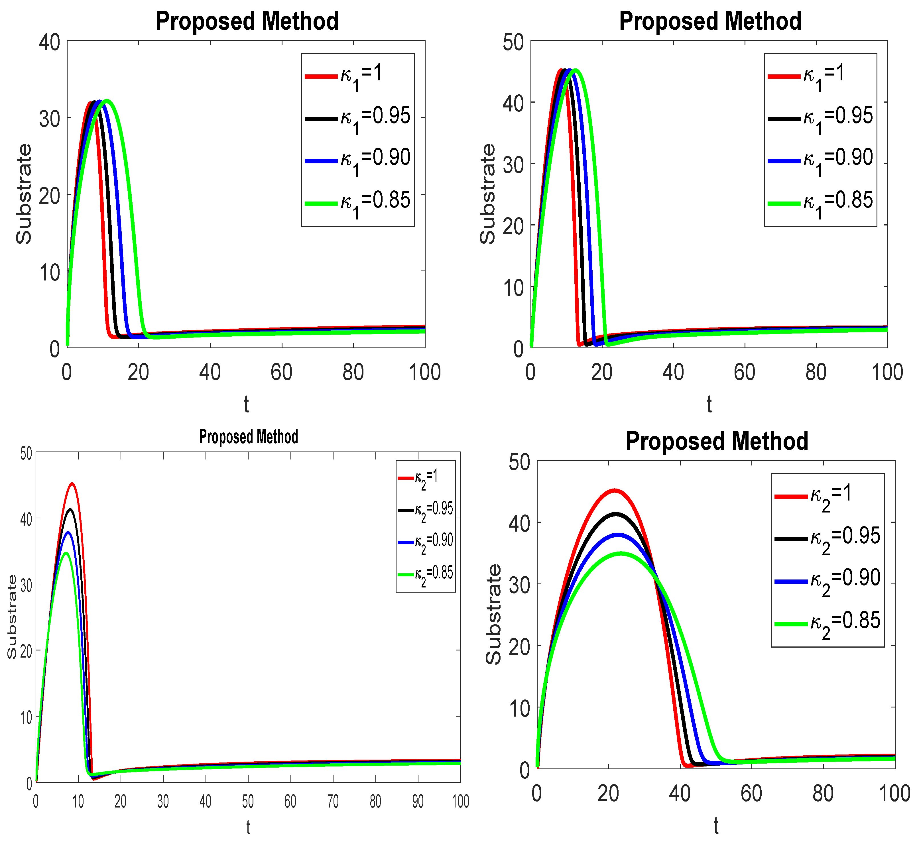
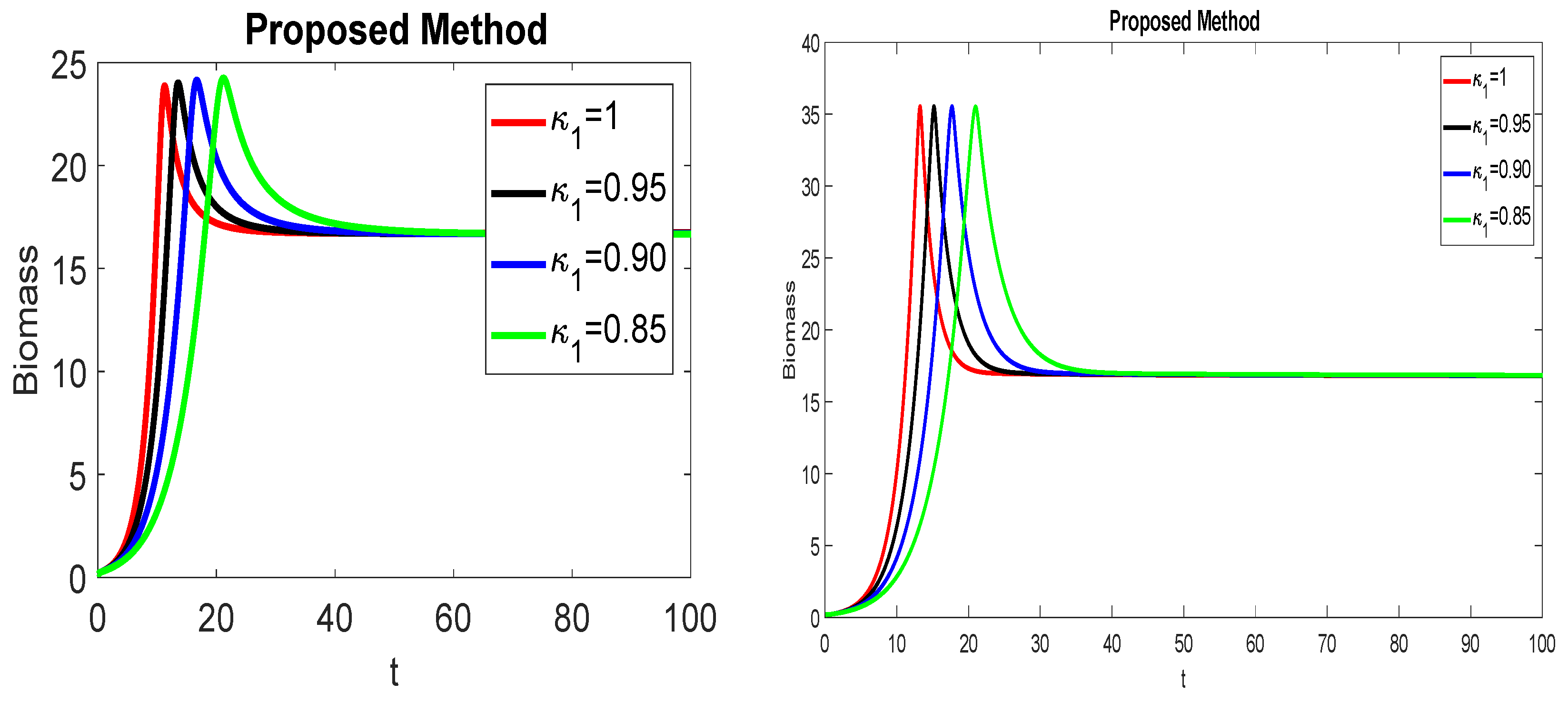
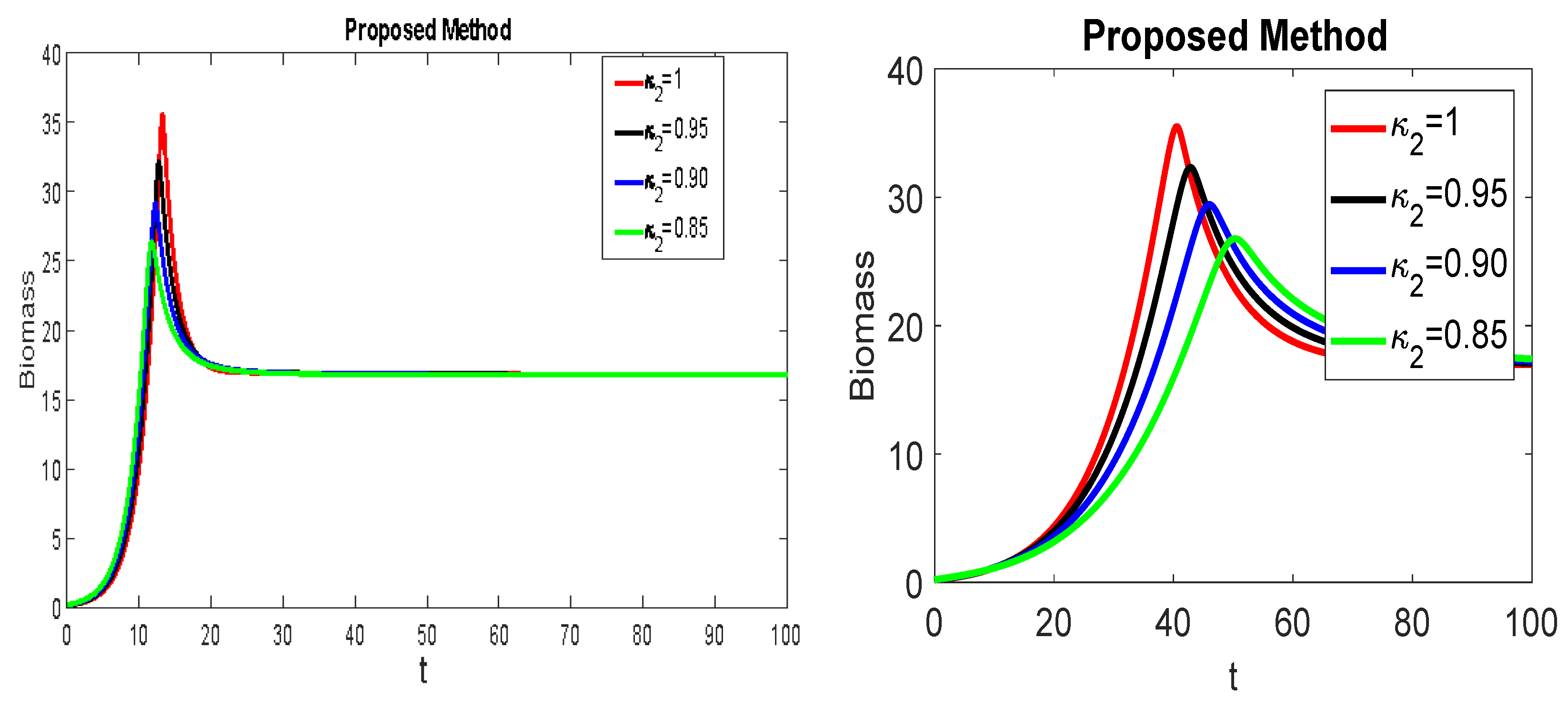
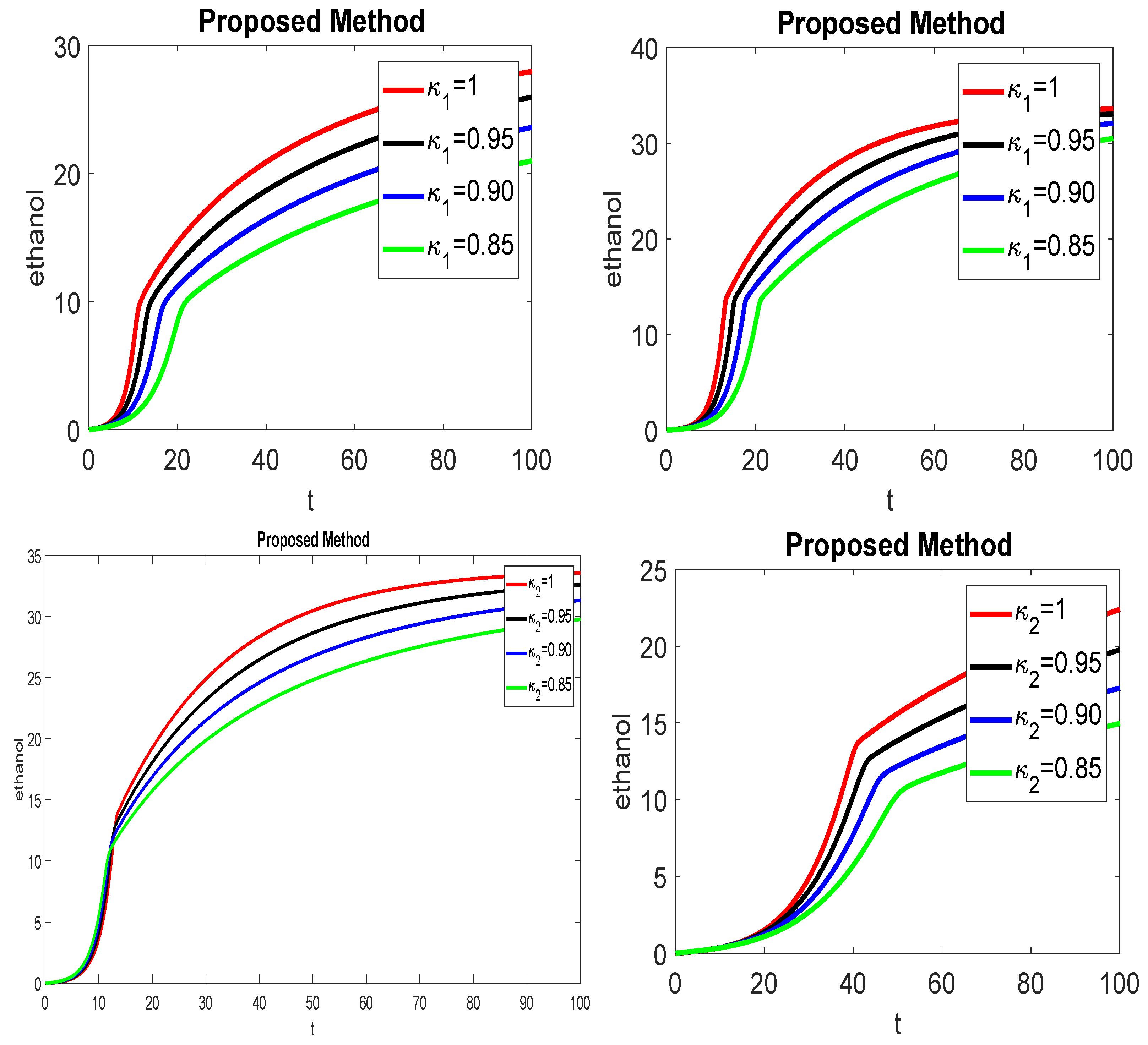
In this section, we simulate the suggested dimensionless nonlinear model using the rate of change of substrate, biomass, and ethanol. To be more specific, we analyze kinetics characteristics with sugar concentrations of 100–250 g/L, which are typically utilized in ethanol production. We use the parameter values and initial conditions for the graphical representation as: $\gamma =0.338$, ${\mu }_{max}=0.333$, ${\mathrm{b}}_{\mathrm{H}}=0.000916$, ${\mathrm{Y}}_{\frac{\mathcal{E}}{\mathcal{X}}}=3.817$, ${\mathrm{Y}}_{\frac{\mathcal{X}}{\mathcal{S}}}=0.054$, ${\mathrm{K}}_{\mathcal{E}}=0.048$, ${\mathrm{K}}_{\mathcal{S}}=0.032$, ${\mathcal{S}}_0^{*}=100$, ${\mathcal{X}}_0^{*}=0.2$, and ${\mathcal{S}}_0^{*}=0$. The values of other parameters used in the dimensionless model are defined as: ${\mathrm{b}}_{\mathrm{H}}^{*}=\frac{{\mathrm{b}}_{\mathrm{H}}}{{\mu }_{max}}$, ${\gamma }_1={\mathrm{K}}_{\mathcal{E}}{\mathrm{K}}_{\mathcal{S}}$, ${\tau }^{*}=\frac{\mathbb{V}{\mu }_{max}}{\mathbb{F}}$, ${\gamma }_2=\gamma {\mathrm{Y}}_{\frac{\mathcal{X}}{\mathcal{S}}}$, and ${\gamma }_3={\mathrm{Y}}_{\frac{\mathcal{E}}{\mathcal{X}}}{\mathrm{Y}}_{\frac{\mathcal{X}}{\mathcal{S}}}$. We illustrate the time evolutions of the substrate, biomass, and ethanol for different choices of ${\kappa }_1$ and ${\kappa }_2$. Figure 1 represents the evolution of the substrate concentration for different values of ${\kappa }_1$ and ${\kappa }_2$. Figure 2 shows the evolution of the biomass concentration for different values of ${\kappa }_1$ and ${\kappa }_2$ while Figure 3 is the graphical representation of the ethanol concentration for various values of ${\kappa }_1$ and ${\kappa }_2$. We consider reactors that have no or continuous substrate, biomass, or ethanol. The abrupt increase generated by the intake of feed concentration can be seen in the Figure 1. Then, bacteria use substrate, due to this, it quickly flattens out to a constant. It is clear from the numbers that using more recycling enhances the generation of biomass and methane. That consequence depletes the substrates required for a successful biorefinery. With a fixed period at t = 100, we see that the substrate concentration rises as the recycling ratio rises. Here we also observe the impact of ${\kappa }_1$ and ${\kappa }_2$ on each other, as shown in Figure 1, Figure 2 and Figure 3. From the first two figures of Figure 1, we observe that varying ${\kappa }_1$ and keeping ${\kappa }_2$ fixed, the substrate concentration attains the one peak value for different values of ${\kappa }_1$. On the other hand, from the last two figures of Figure 1, we see that the substrate concentration attains different peak values at different orders of ${\kappa }_2$, keeping ${\kappa }_1$ fixed. The same is the case for biomass concentration. In Figure 3, the effects of ${\kappa }_1$ and ${\kappa }_2$ on the concentration of ethanol are easily observed. As ${\kappa }_1$ or ${\kappa }_2$ increase, the slower the process of the substrate, biomass, and ethanol and vice versa. When both ${\kappa }_1$ and ${\kappa }_2$ approaches unity, then the curves of the model tend to the curves of the integer-order model. Thus, the generalized fractional-order model provides a global evolution of the substrate, biomass, and ethanol concentration.

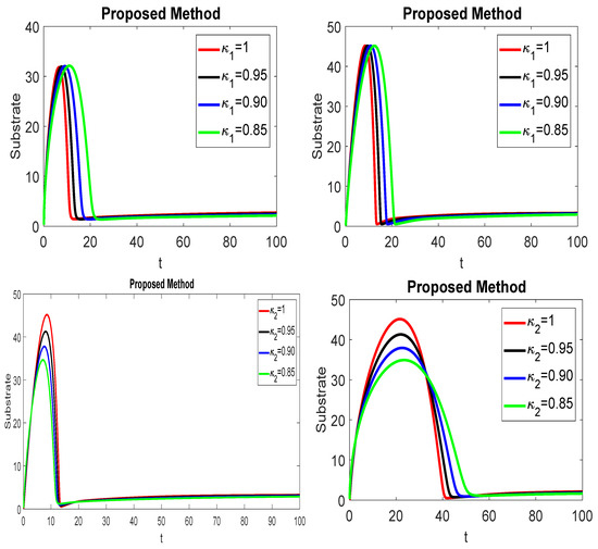
Figure 1. Graphical representation of substrate for different values of ${\kappa }_1$ and ${\kappa }_2$.

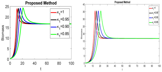
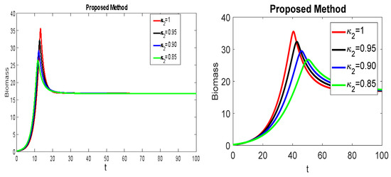
Figure 2. Graphical representation of biomass for different values of ${\kappa }_1$ and ${\kappa }_2$.

Figure 3. Graphical representation of ethanol for different values of ${\kappa }_1$ and ${\kappa }_2$.

6. Conclusions

In this article, we investigated a fractional mathematical model for the synthesis of bio-ethanol using a generalised Caputo operator. We looked into a variety of mathematical properties of the model that are required to support the physical features of the modelled problem. We have presented the applications of well-known results of the Banach and Leray–Schauider fixed point theorems to develop the existence theory regarding at least one unique solution of the considered model. We have discussed different forms of Ulam’s types of stability of the considered model such as UH, generalized UH, URH, and generalized URH. In this study, we have established the algorithm via a numerical method called the predictor–corrector method to find the approximate solution of the dimensionless ethanol model. We have presented the stability of the P–C numerical method. We have shown that the proposed method is conditionally stable. We have geometrically presented the ethanol model under a generalized Caputo operator for different sets of ${\kappa }_1$ and ${\kappa }_2$. We have observed from the graphical representation of the model that the fractional-order ethanol model produces a global evolution of the substrate concentration, biomass concentration, and ethanol concentration. Thus, we conclude that our model is superior to the model given in [10]. In future research, we will study the bifurcation and chaos behavior of the model under various fractional operators.

References

- Kaparaju, P.; Serrano, M.; Thomsen, A.B.; Kongjan, P.; Angelidaki, I. Bioethanol, biohydrogen and biogas production from wheat straw in a biorefinery concept. Bioresour. Technol. 2009, 100, 2562–2568. [Google Scholar] [CrossRef]
- Nigam, P.S.; Singh, A. Production of liquid biofuels from renewable resources. Prog. Energy Combust. Sci. 2011, 37, 52–68. [Google Scholar] [CrossRef]
- Stichnothe, H.; Azapagic, A. Bioethanol from waste: Life cycle estimation of the greenhouse gas saving potential. Resour. Conserv. Recycl. 2011, 53, 624–630. [Google Scholar] [CrossRef]
- Shuler, M.L.; Fikret, K. Bioprocess Engineering: Basic Concepts; Prentice-Hall International: Upper Saddle River, NJ, USA, 2002. [Google Scholar]
- Alqahtani, R.T.; Nelson, M.I.; Worthy, A.L. Analysis of a chemostat model with variable yield coefficient and substrate inhibition: Contois growth kinetics. Chem. Eng. Commun. 2015, 202, 332–344. [Google Scholar] [CrossRef] [Green Version]
- Alqahtani, R.T.; Nelson, M.I.; Worthy, A.L. A biological treatment of industrial wastewaters: Contois kinetics. ANZIAM J. 2015, 56, 397–415. [Google Scholar] [CrossRef]
- Ajbar, A.H. Study of complex dynamics in pure and simple microbial competition. Chem. Eng. Sci. 2012, 80, 188–194. [Google Scholar] [CrossRef]
- Isla, M.A.; Comelli, R.N.; Seluy, L.G. Wastewater from the soft drinks industry as a source for bioethanol production. Bioresour. Technol. 2013, 136, 140–147. [Google Scholar] [CrossRef] [PubMed]
- Comelli, R.N.; Seluy, L.G.; Isla, M.A. Performance of several saccharomyces strains for the alcoholic fermentation of sugar-sweetened high-strength wastewaters: Comparative analysis and kinetic modelling. New Biotechnol. 2016, 33, 874–882. [Google Scholar] [CrossRef]
- Bhowmik, S.K.; Alqahtani, R.T. Mathematical analysis of bioethanol production through continuous reactor with a settling unit. Comput. Chem. Eng. 2018, 111, 241–251. [Google Scholar] [CrossRef]
- Ahmad, S.; Ullah, A.; Akgül, A.; Baleanu, D. Analysis of the fractional tumour-immune-vitamins model with Mittag–Leffler kernel. Results Phys. 2020, 19, 103559. [Google Scholar] [CrossRef]
- Ahmad, S.; Ullah, A.; Shah, K.; Akgül, A. Computational analysis of the third order dispersive fractional PDE under exponential-decay and Mittag-Leffler type kernels. Numer. Methods Partial. Differ. Equ. 2020. [Google Scholar] [CrossRef]
- Kilbas, A.A.; Srivastava, H.H.; Trujillo, J.J. Theory and Applications of Fractional Differential Equations; Elsevier: Amsterdam, The Netherlands, 2006. [Google Scholar]
- Caputo, M.; Fabrizio, M. A new definition of fractional derivative without singular kernel. Prog. Fract. Differ. Appl. 2015, 1, 1–13. [Google Scholar]
- Atangana, A.; Baleanu, D. New fractional derivatives with non-local and non-singular kernel: Theory and application to heat transfer model. Therm. Sci. 2016, 20, 763–769. [Google Scholar] [CrossRef] [Green Version]
- Ahmad, S.; Ullah, A.; Arfan, M.; Shah, K. On analysis of the fractional mathematical model of rotavirus epidemic with the effects of breastfeeding and vaccination under Atangana-Baleanu (AB) derivative. Chaos Solitons Fractals 2020, 140, 110233. [Google Scholar] [CrossRef]
- Ahmad, S.; Ullah, A.; Akgül, A.; De la Sen, M. A study of fractional order Ambartsumian equation involving exponential decay kernel. AIMS Math. 2021, 6, 9981–9997. [Google Scholar] [CrossRef]
- Ullah, A.; Abdeljawad, T.; Ahmad, S.; Shah, K. Study of a fractional-order epidemic model of childhood diseases. J. Funct. Spaces 2020, 2020, 5895310. [Google Scholar] [CrossRef] [PubMed]
- Diethelm, K.; Ford, N.J.; Freed, A.D. A predictor–corrector approach for the numerical solution of fractional differential equations. Nonlinear Dyn. 2002, 29, 3–22. [Google Scholar] [CrossRef]
- Owolabi, K.M.; Atangana, A. Analysis and application of new fractional Adams-Bashforth scheme with Caputo-Fabrizio derivative. Chaos Solitons Fractals 2017, 105, 111–119. [Google Scholar] [CrossRef]
- Shawagfeh, N.T. The decomposition method for fractional differential equations. J. Fract. Calc. 1999, 16, 27–33. [Google Scholar]
- Darania, P.; Ebadian, A. A method for the numerical solution of the integro-differential equations. Appl. Math. Comput. 2007, 188, 657–668. [Google Scholar] [CrossRef]
- Hashim, I.; Abdulaziz, O.; Momani, S. Homotopy analysis method for fractional IVPs. Commun. Nonlinear Sci. Numer. Simul. 2009, 14, 674–684. [Google Scholar] [CrossRef]
- Katugampola, U.N. A new approach to generalized fractional derivatives. Bull. Math. Anal. Appl. 2014, 6, 1–15. [Google Scholar]
- Katugampola, U.N. New approach to generalized fractional integral. Appl. Math. Comput. 2011, 218, 860–865. [Google Scholar] [CrossRef] [Green Version]
- Odibat, Z.; Baleanu, D. Numerical simulation of initial value problems with generalized Caputotype fractional derivatives. Appl. Numer. Math. 2020, 156, 94–105. [Google Scholar] [CrossRef]
- Kumar, P.; Erturk, V.S.; Murillo-Arcila, M. A complex fractional mathematical modeling for the love story of Layla and Majnun. Chaos Solitons Fractals 2021, 150, 111091. [Google Scholar] [CrossRef]
- Kongson, J.; Thaiprayoon, C.; Sudsutad, W. Analysis of a fractional model for HIV CD4+ T-cells with treatment under generalized Caputo fractional derivative. AIMS Math. 2021, 6, 7285–7304. [Google Scholar] [CrossRef]
- Asl, M.S.; Javidi, M. An improved PC scheme for nonlinear fractional differential equations: Error and stability analysis. J. Comput. Appl. Math. 2017, 324, 101–117. [Google Scholar] [CrossRef]
- Garrappa, R. On some explicit Adams multistep methods for fractional differential equations. J. Comput. Appl. Math. 2009, 299, 392–399. [Google Scholar] [CrossRef] [Green Version]
- Odibat, Z.; Shawagfeh, N. An optimized linearization-based predictor–corrector algorithm for the numerical simulation of nonlinear FDEs. Phys. Scr. 2020, 95, 065202. [Google Scholar] [CrossRef]
- Garrappa, R. Numerical Solution of Fractional Differential Equations: A Survey and a Software Tutorial. Mathematics 2018, 6, 16. [Google Scholar] [CrossRef] [Green Version]
Publisher’s Note: MDPI stays neutral with regard to jurisdictional claims in published maps and institutional affiliations. |
© 2021 by the authors. Licensee MDPI, Basel, Switzerland. This article is an open access article distributed under the terms and conditions of the Creative Commons Attribution (CC BY) license (https://creativecommons.org/licenses/by/4.0/).