Limiting Genotype Frequencies of Y-Linked Genes with a Mutant Allele in a Two-Sex Population

Abstract

A two-type two-sex branching process is considered to model the evolution of the number of carriers of an allele and its mutations of a Y-linked gene. The limiting growth rates of the different types of couples and males (depending on the allele, mutated or not, that they carry on) on the set of coexistence of both alleles and on the fixation set of the mutant allele are obtained. In addition, the limiting genotype of the Y-linked gene and the limiting sex frequencies on those sets are established. Finally, the main results have been illustrated with simulated studies contextualized in problems of population genetics.

1. Introduction

In many populations, the sex of an individual is determined by a pair of chromosomes X and Y. The females are homozygous and carry $XX$ chromosomes, the males are heterozygous and carry $XY$ chromosomes. Sex-linkage occurs if the phenotypic expression of an allele is related to the chromosomal sex of the individual. Here we are interested in Y-linkage. Although there are much less Y-linked traits than X-linked traits, recent studies have shown the significance of Y-linkage in the biology of humans and other animals, see e.g., [1]. A mathematical model for the propagation of Y-linked genes in two-sex populations was introduced by González et al. [2] and further studied in [3,4]. The genes occur in two allelic forms, called $\mathsf{R}$ and $\mathsf{r}$, where the latter one cannot mutate, the mating is assumed to be monogamous (perfect fidelity mating) and with blind choice, that is, females ignore or do not care about the genotype of the chosen partner.

In this paper we consider the model just outlined but with the additional possibility of mutations. Such a model was introduced in González et al. [5]. More precisely, in this paper it is assumed that $\mathsf{R}$ represents the nonmutant allelic form of the gene which can mutate and thus give rise to new allelic forms, all of them denoted by $\mathsf{r}$ and called mutant alleles. Although the latter can also mutate this is ignored in this case because we do not further distinguish between possible types of mutation, and a reversion, i.e., a mutation from $\mathsf{r}$ back to $\mathsf{R}$, is not allowed. In such paper, conditions for the extinction and survival of those alleles were studied and also further biological information that explain the relevance of mutations in this context were provided. Furthermore, inference on the main parameters of the model was made in [6].

The aim of this work is to find the allele growth rates as well as the limiting genotype and sex frequencies for such a model in the supercritical case (in terms of the usual nomenclature used in branching processes theory). Particularly, the growth rate of the mutant allele on its fixation set and the one of the nonmutant allele on the coexistence set are obtained. Also on that set of coexistence, the growth rate of the mutant allele is studied. However, in this case, mutant allele survival depends on the behaviour of the nonmutant allele, and this fact makes this study more complex. The obtained results depend on the relation between the means of the offspring distributions of the different genotypes (with mutant or nonmutant alleles) and the probability of mutation. Finally, we illustrate the attained results by way of simulated studies contextualised in problems of population genetics, such as the evolution of infertility problems in males, the existence of degeneration of Y chromosome or the possibility of diversity of species without natural selection.

We have split the paper into eight sections. In Section 2 we provide a mathematical description of the model. Then, in Section 3, we research the limiting growth rate of the nonmutant allele. Next, we found the rate of growth of the mutant allele on the coexistence set and also on its fixation set, in Section 4. As consequence, in Section 5, we deal with the limiting genotype and sex frequencies. Illustrative examples are shown in Section 6. Finally, in Section 7 some concluding remarks are given and the paper ends with an Appendix which contains the proofs of the results provided throughout the paper.

2. Model Description

A detailed description of the mathematical model is provided next: individuals are called females, $\mathsf{R}$-males (males with $\mathsf{R}$-genotype) and $\mathsf{r}$-males (males with $\mathsf{r}$-genotype), and these can mate with females to form $\mathsf{R}$- or $\mathsf{r}$-couples depending on whether the male is of type $\mathsf{R}$ or $\mathsf{r}$, respectively. In accordance with the rules of genetic inheritance and by taking the possibility of mutation into account, an $\mathsf{R}$-couple can give birth to females, $\mathsf{R}$-males, and $\mathsf{r}$-males, whereas, given the assumption of no backmutation, an $\mathsf{r}$-couple gives birth to females and $\mathsf{r}$-males.

Assuming nonoverlapping generations and given the number of $\mathsf{R}$- and $\mathsf{r}$-couples in generation $\mathsf{n}$, denoted by ${\mathsf{Z}}_{\mathsf{n}}^{\mathsf{R}}$ and ${\mathsf{Z}}_{\mathsf{n}}^{\mathsf{r}}$, respectively, the numbers of females, males, and couples of each genotype in the next generation are determined by the following two-stage procedure of reproduction and mating:

In the reproduction phase, couples produce offspring independent of each other and in accordance with an offspring law which does not depend on the generation, is the same for a given genotype, but may vary for different genotypes since the mutation could affect the reproductive capacity. Formally, the numbers of females and males produced by the couples of type $\mathsf{R}$ and $\mathsf{r}$ are determined by sequences of independent, identically distributed (i.i.d.) random vectors, viz.

$$({\mathsf{F}}_{\mathsf{ni}}^{\mathsf{R}},{\mathsf{M}}_{\mathsf{ni}}^{\mathsf{R}},{\mathsf{M}}_{\mathsf{ni}}^{\mathsf{R}\to \mathsf{r}})\mathrm{and}({\mathsf{F}}_{\mathsf{ni}}^{\mathsf{r}},{\mathsf{M}}_{\mathsf{ni}}^{\mathsf{r}\to \mathsf{r}}),(\mathsf{n},\mathsf{i})\in {\mathbb{N}}_0\times \mathbb{N},$$

respectively. Here, ${\mathsf{F}}_{\mathsf{ni}}^{\mathsf{x}}$ denotes the number of female offspring of the $\mathsf{i}$th $\mathsf{x}$-couple in generation $\mathsf{n}$ with $\mathsf{x}\in \{\mathsf{R},\mathsf{r}\}$, while ${\mathsf{M}}_{\mathsf{ni}}^{\mathsf{R}}$ and ${\mathsf{M}}_{\mathsf{ni}}^{\mathsf{r}\to \mathsf{r}}$ denote the numbers of nonmutant male offspring of the $\mathsf{i}$th $\mathsf{R}$ and $\mathsf{r}$-couples, respectively, in generation $\mathsf{n}$, and ${\mathsf{M}}_{\mathsf{ni}}^{\mathsf{R}\to \mathsf{r}}$ denotes the number of mutant males produce by the $\mathsf{i}$th $\mathsf{R}$-couple in generation $\mathsf{n}$. All variables are assumed to have finite mean and variance, and we denote

$${\mathsf{m}}_{\mathsf{R}}=E[{\mathsf{F}}_{\mathsf{ni}}^{\mathsf{R}}+{\mathsf{M}}_{\mathsf{ni}}^{\mathsf{R}}+{\mathsf{M}}_{\mathsf{ni}}^{\mathsf{R}\to \mathsf{r}}]\mathrm{and}{\mathsf{m}}_{\mathsf{r}}=E[{\mathsf{F}}_{\mathsf{ni}}^{\mathsf{r}}+{\mathsf{M}}_{\mathsf{ni}}^{\mathsf{r}\to \mathsf{r}}].$$

Furthermore, the conditional law of $({\mathsf{F}}_{\mathsf{ni}}^{\mathsf{R}},{\mathsf{M}}_{\mathsf{ni}}^{\mathsf{R}},{\mathsf{M}}_{\mathsf{ni}}^{\mathsf{R}\to \mathsf{r}})$ given ${\mathsf{F}}_{\mathsf{ni}}^{\mathsf{R}}+{\mathsf{M}}_{\mathsf{ni}}^{\mathsf{R}}+{\mathsf{M}}_{\mathsf{ni}}^{\mathsf{R}\to \mathsf{r}}=\mathsf{k}$, $\mathsf{k}\ge 0$, is assumed to be multinomial with parameters $\mathsf{k}$, $\alpha$, $(1-\alpha )(1-\beta )$ and $(1-\alpha )\beta$ and the conditional law of $({\mathsf{F}}_{\mathsf{ni}}^{\mathsf{r}},{\mathsf{M}}_{\mathsf{ni}}^{\mathsf{r}\to \mathsf{r}})$ given ${\mathsf{F}}_{\mathsf{ni}}^{\mathsf{r}}+{\mathsf{M}}_{\mathsf{ni}}^{\mathsf{r}\to \mathsf{r}}=\mathsf{k}$, $\mathsf{k}\ge 0$, to be multinomial with parameters $\mathsf{k}$, $\alpha$, $(1-\alpha )$. This means that $\alpha$ equals the probability that an offspring is female, while $\beta$ equals the probability that a newborn male of an $\mathsf{R}$-couple has the mutant allele. At the end of the reproduction phase, one has ${\mathsf{F}}_{\mathsf{n}+\mathsf{1}}$, ${\mathsf{M}}_{\mathsf{n}+\mathsf{1}}^{\mathsf{R}}$, and ${\mathsf{M}}_{\mathsf{n}+\mathsf{1}}^{\mathsf{r}}$, the total numbers of females, $\mathsf{R}$-males, and $\mathsf{r}$-males, respectively, which constitute the generation $\mathsf{n}+\mathsf{1}$ and they are determined by the following relations (with the empty sum defined as 0):

$${\mathsf{F}}_{\mathsf{n}+\mathsf{1}}=\sum _{\mathsf{i}=1}^{{\mathsf{Z}}_{\mathsf{n}}^{\mathsf{R}}}{\mathsf{F}}_{\mathsf{ni}}^{\mathsf{R}}+\sum _{\mathsf{j}=1}^{{\mathsf{Z}}_{\mathsf{n}}^{\mathsf{r}}}{\mathsf{F}}_{\mathsf{nj}}^{\mathsf{r}},$$

$${\mathsf{M}}_{\mathsf{n}+\mathsf{1}}^{\mathsf{R}}=\sum _{\mathsf{i}=1}^{{\mathsf{Z}}_{\mathsf{n}}^{\mathsf{R}}}{\mathsf{M}}_{\mathsf{ni}}^{\mathsf{R}}\mathrm{and}{\mathsf{M}}_{\mathsf{n}+\mathsf{1}}^{\mathsf{r}}={\mathsf{M}}_{\mathsf{n}+\mathsf{1}}^{\mathsf{R}\to \mathsf{r}}+{\mathsf{M}}_{\mathsf{n}+\mathsf{1}}^{\mathsf{r}\to \mathsf{r}},$$

(1)

where

$${\mathsf{M}}_{\mathsf{n}+\mathsf{1}}^{\mathsf{R}\to \mathsf{r}}=\sum _{\mathsf{i}=1}^{{\mathsf{Z}}_{\mathsf{n}}^{\mathsf{R}}}{\mathsf{M}}_{\mathsf{ni}}^{\mathsf{R}\to \mathsf{r}}\mathrm{and}{\mathsf{M}}_{\mathsf{n}+\mathsf{1}}^{\mathsf{r}\to \mathsf{r}}=\sum _{\mathsf{j}=1}^{{\mathsf{Z}}_{\mathsf{n}}^{\mathsf{r}}}{\mathsf{M}}_{\mathsf{nj}}^{\mathsf{r}\to \mathsf{r}}.$$

Thus, ${\mathsf{M}}_{\mathsf{n}+\mathsf{1}}^{\mathsf{R}\to \mathsf{r}}$ and ${\mathsf{M}}_{\mathsf{n}+\mathsf{1}}^{\mathsf{r}\to \mathsf{r}}$ denote the total number of $\mathsf{r}$-males stemming from $\mathsf{R}$- and $\mathsf{r}$-couples in generation $\mathsf{n}$, respectively. Moreover, we denote ${\mathsf{Z}}_{\mathsf{n}}={\mathsf{Z}}_{\mathsf{n}}^{\mathsf{R}}+{\mathsf{Z}}_{\mathsf{n}}^{\mathsf{r}}$ to the total number of couples in generation $\mathsf{n}$.

In the mating phase the number of couples of each genotype, that is ${\mathsf{Z}}_{\mathsf{n}+\mathsf{1}}^{\mathsf{R}}$ and ${\mathsf{Z}}_{\mathsf{n}+\mathsf{1}}^{\mathsf{r}}$, are determined as follows, given the total number of females, $\mathsf{R}$-males and $\mathsf{r}$-males in generation $\mathsf{n}+1$. We assume monogamous mating which means that the total number of couples equals the minimum of ${\mathsf{F}}_{\mathsf{n}+\mathsf{1}}$ and ${\mathsf{M}}_{\mathsf{n}+\mathsf{1}}={\mathsf{M}}_{\mathsf{n}+\mathsf{1}}^{\mathsf{R}}+{\mathsf{M}}_{\mathsf{n}+\mathsf{1}}^{\mathsf{r}}$. In the case when ${\mathsf{F}}_{\mathsf{n}+\mathsf{1}}\ge {\mathsf{M}}_{\mathsf{n}+\mathsf{1}}$, this means that each male finds a female to mate with, i.e., ${\mathsf{Z}}_{\mathsf{n}+\mathsf{1}}^{\mathsf{R}}={\mathsf{M}}_{\mathsf{n}+\mathsf{1}}^{\mathsf{R}}$ and ${\mathsf{Z}}_{\mathsf{n}+\mathsf{1}}^{\mathsf{r}}={\mathsf{M}}_{\mathsf{n}+\mathsf{1}}^{\mathsf{r}}$. In the case when ${\mathsf{F}}_{\mathsf{n}+\mathsf{1}}<{\mathsf{M}}_{\mathsf{n}+\mathsf{1}}$, females must choose a partner. We assume that this is done without preference of the genotype (blind choice). As a consequence, the conditional law of the total number of $\mathsf{x}$-couples ${\mathsf{Z}}_{\mathsf{n}+\mathsf{1}}^{\mathsf{x}}$ given (${\mathsf{F}}_{\mathsf{n}+\mathsf{1}},{\mathsf{M}}_{\mathsf{n}+\mathsf{1}}^{\mathsf{R}},{\mathsf{M}}_{\mathsf{n}+\mathsf{1}}^{\mathsf{r}})$ is hypergeometric with parameters (${\mathsf{F}}_{\mathsf{n}+\mathsf{1}},{\mathsf{M}}_{\mathsf{n}+\mathsf{1}},{\mathsf{M}}_{\mathsf{n}+\mathsf{1}}^{\mathsf{x}})$ with $\mathsf{x}\in \{\mathsf{R},\mathsf{r}\}$.

The bivariate sequence ${\left\{({\mathsf{Z}}_{\mathsf{n}}^{\mathsf{R}},{\mathsf{Z}}_{\mathsf{n}}^{\mathsf{r}})\right\}}_{\mathsf{n}\ge 0}$ describing the evolution of the number of couples for each type of males over generations is called Y-linked two-sex branching process with mutations, fidelity mating and blind choice of males. As shown in [5], it is a temporally homogeneous multitype Markov chain and exhibits the extinction-explosion dichotomy which is usual for branching processes with independent reproduction.

Notice that, since the empty sum is assumed to be zero, if in some generation there are no mating units of type $\mathsf{R}$ then, from this generation on, the couples and males of that type as well as mutant-males coming from them no longer exist, that is, if ${\mathsf{Z}}_{\mathsf{n}}^{\mathsf{R}}=0$ for some $\mathsf{n}>0$, then ${\mathsf{Z}}_{\mathsf{k}}^{\mathsf{R}}=0$, ${\mathsf{M}}_{\mathsf{k}}^{\mathsf{R}}=0$ and ${\mathsf{M}}_{\mathsf{k}}^{\mathsf{R}\to \mathsf{r}}=0$ for all $\mathsf{k}>\mathsf{n}$. Also, if ${\mathsf{Z}}_{\mathsf{n}}^{\mathsf{R}}=0$ and ${\mathsf{Z}}_{\mathsf{n}}^{\mathsf{r}}=0$ for some $\mathsf{n}>0$, then ${\mathsf{Z}}_{\mathsf{k}}^{\mathsf{r}}=0$ and ${\mathsf{M}}_{\mathsf{k}}^{\mathsf{r}}=0$ for all $\mathsf{k}>\mathsf{n}$. However, this behaviour is different for the $\mathsf{r}$-allele when ${\mathsf{Z}}_{\mathsf{n}}^{\mathsf{R}}\ne 0$. Indeed, despite ${\mathsf{Z}}_{\mathsf{n}}^{\mathsf{r}}=0$, it could happen that some $\mathsf{R}$-couple gives birth to males whose corresponding allele has suffered a mutation and some of these males could mate forming couples of type $\mathsf{r}$. Hence, if ${\mathsf{Z}}_{\mathsf{n}}^{\mathsf{R}}\ne 0$, one can find that ${\mathsf{M}}_{\mathsf{k}}^{\mathsf{r}}>0$ and ${\mathsf{Z}}_{\mathsf{k}}^{\mathsf{r}}>0$, for some $\mathsf{k}>\mathsf{n}$, even being ${\mathsf{Z}}_{\mathsf{n}}^{\mathsf{r}}=0$. Taking into account this fact, in [5] was shown that the survival of the population over generations is determined by the two events $\{{\mathsf{Z}}_{\mathsf{n}}^{\mathsf{R}}\to 0,{\mathsf{Z}}_{\mathsf{n}}^{\mathsf{r}}\to \infty \}$, termed $\mathsf{r}$-fixation, and $\{{\mathsf{Z}}_{\mathsf{n}}^{\mathsf{R}}\to \infty ,{\mathsf{Z}}_{\mathsf{n}}^{\mathsf{r}}\to \infty \}=\{{\mathsf{Z}}_{\mathsf{n}}^{\mathsf{R}}\to \infty \}$ almost surely (a.s.), termed simultaneous survival of both genotypes or coexistence, that is, the survival of $\mathsf{R}$-genotype implies also the survival of $\mathsf{r}$-genotype.

The following sections are devoted to the study of asymptotic growth of each genotype on survival events (in the usually called supercritical case). In all of them we shall write $P_{(\mathsf{i},\mathsf{j})}(·)$ for $P(·|{\mathsf{Z}}_{\mathsf{0}}^{\mathsf{R}}=\mathsf{i},{\mathsf{Z}}_{\mathsf{0}}^{\mathsf{r}}=\mathsf{j})$ or even the index $(\mathsf{i},\mathsf{j})$ will be dropped in the notation if there is no ambiguity. To end this section, it is worth mentioning that detailed investigation of some particular two-type branching processes beyond the general theory has been also developed in other settings as, for example, in [7].

3. Nonmutant Allele Growth Rate

Next, we assume that $(\alpha \wedge (1-\alpha ))(1-\beta ){\mathsf{m}}_{\mathsf{R}}>1$, where, recall that $(1-\alpha )(1-\beta ){\mathsf{m}}_{\mathsf{R}}$ is the mean number of $\mathsf{R}$-males per $\mathsf{R}$-couple and $\alpha (1-\beta ){\mathsf{m}}_{\mathsf{R}}$ can be interpreted as the mean number of females produced by $\mathsf{R}$-couples who mate with $\mathsf{R}$-males. Under this condition, it was proved in [5] that the survival of $\mathsf{R}$-genotype (equivalently, simultaneous survival of both genotypes) occurs with positive probability. It then makes, to determine in this case, the limiting growth rates for the number of $\mathsf{R}$-couples and $\mathsf{R}$-males. Answer is provided by the following result.

Theorem 1.

Let ${\tau }_{\mathsf{R}}=(\alpha \wedge (1-\alpha ))(1-\beta ){\mathsf{m}}_{\mathsf{R}}$. If ${\tau }_{\mathsf{R}}>1$, then there exists a random variable ${\mathsf{W}}_{\mathsf{R}}$ which is positive and finite on $\{{\mathsf{Z}}_{\mathsf{n}}^{\mathsf{R}}\to \infty \}$, such that

$$\underset{\mathsf{n}\to \infty }{lim}\frac{{\mathsf{Z}}_{\mathsf{n}}^{\mathsf{R}}}{{\tau }_{\mathsf{R}}^{\mathsf{n}}}={\mathsf{W}}_{\mathsf{R}}and\underset{\mathsf{n}\to \infty }{lim}\frac{{\mathsf{M}}_{\mathsf{n}}^{\mathsf{R}}}{{\tau }_{\mathsf{R}}^{\mathsf{n}}}=\frac{(1-\alpha )(1-\beta ){\mathsf{m}}_{\mathsf{R}}}{{\tau }_{\mathsf{R}}}{\mathsf{W}}_{\mathsf{R}} a.s.on \{{\mathsf{Z}}_{\mathsf{n}}^{\mathsf{R}}\to \infty \}.$$

Intuitively speaking, this theorem establishes that the numbers of $\mathsf{R}$-couples and $\mathsf{R}$-males grow geometrically at the rate given by the mean number of nonmutant males generated by an $\mathsf{R}$-couple or by the mean number of females stemming from an $\mathsf{R}$-couple who mate with nonmutant males, respectively, depending on whether $\alpha$ is higher than 0.5 or not.

4. Mutant Allele Growth Rate

Firstly, we consider the study of the rate of growth of the process ${\left\{{\mathsf{Z}}_{\mathsf{n}}^{\mathsf{r}}\right\}}_{\mathsf{n}\ge 0}$ on the event of coexistence, that is on $\{{\mathsf{Z}}_{\mathsf{n}}^{\mathsf{R}}\to \infty \}$. This study turns out to be more difficult than the previous case because of the possible dependency of the survival of the $\mathsf{r}$-allele on the behaviour of the $\mathsf{R}$-allele. In fact, from the previous result, it is easy to deduce that $\mathsf{r}$-males stemming from $\mathsf{R}$-couples grow geometrically at the same rate as $\mathsf{R}$-males. To carry out this study, we again assume that $(\alpha \wedge (1-\alpha ))(1-\beta ){\mathsf{m}}_{\mathsf{R}}>1$ and distinguish two cases: when $\alpha >0.5$ and when $\alpha \le 0.5$, in order to better understanding. Finally, we consider the study on $\mathsf{r}$-fixation set.

4.1. On Coexistence Set: Case $\alpha >0.5$

When $\alpha >0.5$, the number of females always exceeds the number of males from some generation onwards on the set of survival of both genotypes (see Corollary A.1 in [5]). Then, eventually, the number of each type of couple equals the number of males of each genotype. Therefore, the process behaves essentially as a two-type Galton–Watson process where one of the types ($\mathsf{R}$-allele) gives birth the two types of individuals existing in the population ($\mathsf{R}$-males and $\mathsf{r}$-males) while the other type ($\mathsf{r}$-allele) only produces individuals of its own type ($\mathsf{r}$-males). For more details, the reader is referred to the state-space representation in page 10 of the Appendix A. The limit theorems for a reducible multitype Galton–Watson process (as it is our case) are well studied in [8] and can be applied here to obtain the following theorem.

Theorem 2.

If $\alpha >0.5$ and $(1-\alpha )(1-\beta ){\mathsf{m}}_{\mathsf{R}}>1$, then there exists a random variable ${\mathsf{W}}_{\mathsf{r}}$ which is positive and finite on $\{{\mathsf{Z}}_{\mathsf{n}}^{\mathsf{R}}\to \infty \}$, such that, a.s. on $\{{\mathsf{Z}}_{\mathsf{n}}^{\mathsf{R}}\to \infty \}$,

(i) 

if ${\mathsf{m}}_{\mathsf{r}}>(1-\beta ){\mathsf{m}}_{\mathsf{R}}$, then ${\displaystyle {\displaystyle \underset{\mathsf{n}\to \infty }{lim}\frac{{\mathsf{Z}}_{\mathsf{n}}^{\mathsf{r}}}{{\left((1-\alpha ){\mathsf{m}}_{\mathsf{r}}\right)}^{\mathsf{n}}}=\underset{\mathsf{n}\to \infty }{lim}\frac{{\mathsf{M}}_{\mathsf{n}}^{\mathsf{r}}}{{\left((1-\alpha ){\mathsf{m}}_{\mathsf{r}}\right)}^{\mathsf{n}}}={\mathsf{W}}_{\mathsf{r}}}}$,

(ii) 

if ${\mathsf{m}}_{\mathsf{r}}=(1-\beta ){\mathsf{m}}_{\mathsf{R}}$, then ${\displaystyle {\displaystyle \underset{\mathsf{n}\to \infty }{lim}\frac{{\mathsf{Z}}_{\mathsf{n}}^{\mathsf{r}}}{\mathsf{n}{\left((1-\alpha ){\mathsf{m}}_{\mathsf{r}}\right)}^{\mathsf{n}}}=\underset{\mathsf{n}\to \infty }{lim}\frac{{\mathsf{M}}_{\mathsf{n}}^{\mathsf{r}}}{\mathsf{n}{\left((1-\alpha ){\mathsf{m}}_{\mathsf{r}}\right)}^{\mathsf{n}}}=\frac{\beta }{1-\beta }{\mathsf{W}}_{\mathsf{R}}}}$,

(iii) 

if ${\mathsf{m}}_{\mathsf{r}}<(1-\beta ){\mathsf{m}}_{\mathsf{R}}$, then ${\displaystyle \underset{\mathsf{n}\to \infty }{lim}\frac{{\mathsf{Z}}_{\mathsf{n}}^{\mathsf{r}}}{{\left((1-\alpha )(1-\beta ){\mathsf{m}}_{\mathsf{R}}\right)}^{\mathsf{n}}}=\underset{\mathsf{n}\to \infty }{lim}\frac{{\mathsf{M}}_{\mathsf{n}}^{\mathsf{r}}}{{\left((1-\alpha )(1-\beta ){\mathsf{m}}_{\mathsf{R}}\right)}^{\mathsf{n}}}=\gamma {\mathsf{W}}_{\mathsf{R}},}$

with ${\mathsf{W}}_{\mathsf{R}}$ as in Theorem 1 and ${\displaystyle \gamma =\frac{\beta {\mathsf{m}}_{\mathsf{R}}}{(1-\beta ){\mathsf{m}}_{\mathsf{R}}-{\mathsf{m}}_{\mathsf{r}}}}$.

Notice that, in the previous results it is shown that the rate of growth of ${\left\{{\mathsf{Z}}_{\mathsf{n}}^{\mathsf{r}}\right\}}_{\mathsf{n}>0}$ (and also the rate of growth of ${\left\{{\mathsf{M}}_{\mathsf{n}}^{\mathsf{r}}\right\}}_{\mathsf{n}>0}$) changes depending on the relation between ${\mathsf{m}}_{\mathsf{r}}$ (the mean number of offspring per $\mathsf{r}$-couple) and $(1-\beta ){\mathsf{m}}_{\mathsf{R}}$ (the mean number of offspring per $\mathsf{R}$-couples related with $\mathsf{R}$-allele). In fact, when ${\mathsf{m}}_{\mathsf{r}}>(1-\beta ){\mathsf{m}}_{\mathsf{R}}$ its asymptotic growth is geometric being the rate of growth the mean number of males stemming from $\mathsf{r}-$couples. On the other hand, when ${\mathsf{m}}_{\mathsf{r}}=(1-\beta ){\mathsf{m}}_{\mathsf{R}}$, the normalized sequence is ${\left\{\mathsf{n}{\left((1-\alpha ){\mathsf{m}}_{\mathsf{r}}\right)}^{\mathsf{n}}\right\}}_{\mathsf{n}>0}={\left\{\mathsf{n}{\left((1-\alpha )(1-\beta ){\mathsf{m}}_{\mathsf{R}}\right)}^{\mathsf{n}}\right\}}_{\mathsf{n}>0}$. However, when ${\mathsf{m}}_{\mathsf{r}}<(1-\beta ){\mathsf{m}}_{\mathsf{R}}$, the growth of the $\mathsf{r}$-allele is mainly (at least in part or totally when ${\mathsf{m}}_{\mathsf{r}}=0$) due to the mutations. For that, its asymptotic growth is geometric with rate given by the mean number of males produced by $\mathsf{R}$-couples (the same rate as $\mathsf{R}$-allele (see Theorem 1)). Therefore, when ${\mathsf{m}}_{\mathsf{r}}\ge (1-\beta ){\mathsf{m}}_{\mathsf{R}}$, the $\mathsf{r}$-allele is the dominant one in the population (in the sense that eventually there are more males in the population with $\mathsf{r}$-genotype that with $\mathsf{R}$-genotype).

4.2. On Coexistence Set: Case $\alpha \le 0.5$

Now, when $\alpha <0.5$, the number of males is eventually higher than the number of females (see Corollary A.1 in [5]). Then, in this case, the total numbers of couples of each type are distributed according to hypergeometric distributions. Therefore, the process ${\left\{({\mathsf{Z}}_{\mathsf{n}}^{\mathsf{R}},{\mathsf{Z}}_{\mathsf{n}}^{\mathsf{r}})\right\}}_{\mathsf{n}\ge 0}$ cannot be seen as a multitype branching process as in the previous case. Moreover, in the boundary case, $\alpha =0.5$, we have an oscillating situation where we cannot assert that eventually the number of females (or males) is higher than the number of males (or females) from one generation onward. These two statements make the case $\alpha \le 0.5$ to be more complicated to study from a mathematical point of view than the case $\alpha >0.5$, although we can establish similar results to such given in Theorem 2.

In particular, it can be proved that when $\alpha \le 0.5$ and ${\mathsf{m}}_{\mathsf{r}}<(1-\beta ){\mathsf{m}}_{\mathsf{R}}$, the asymptotic growth of the total number of $\mathsf{r}$-couples is geometric being the growth rate the mean number of females stemming from $\mathsf{R}$-couples who have mated with $\mathsf{R}$-males, that is $\alpha (1-\beta ){\mathsf{m}}_{\mathsf{R}}$ (the same rate as $\mathsf{R}$-allele, see Theorem 1), while than, when ${\mathsf{m}}_{\mathsf{r}}>(1-\beta ){\mathsf{m}}_{\mathsf{R}}$, it is also geometric, but now being the rate of growth the mean number of females stemming from $\mathsf{r}$-couples, that is $\alpha {\mathsf{m}}_{\mathsf{r}}$. The case ${\mathsf{m}}_{\mathsf{r}}=(1-\beta ){\mathsf{m}}_{\mathsf{R}}$ is special, being the normalised sequence ${\left\{\mathsf{n}{\left(\alpha {\mathsf{m}}_{\mathsf{r}}\right)}^{\mathsf{n}}\right\}}_{\mathsf{n}>0}={\left\{\mathsf{n}{\left(\alpha (1-\beta ){\mathsf{m}}_{\mathsf{R}}\right)}^{\mathsf{n}}\right\}}_{\mathsf{n}>0}$, since in each generation $\mathsf{R}$-couples can produce $\mathsf{r}$-males and this partial pedigree grows geometrically at rate given by $\alpha {\mathsf{m}}_{\mathsf{r}}$ (the mean number of females stemming from $\mathsf{r}$-couple).

Theorem 3.

If $\alpha \le 0.5$ and $\alpha (1-\beta ){\mathsf{m}}_{\mathsf{R}}>1$, then there exists a random variable ${\mathsf{W}}_{\mathsf{r}}^{*}$ which is positive and finite on $\{{\mathsf{Z}}_{\mathsf{n}}^{\mathsf{R}}\to \infty \}$, such that, a.s. on $\{{\mathsf{Z}}_{\mathsf{n}}^{\mathsf{R}}\to \infty \}$,

(i) 

if ${\mathsf{m}}_{\mathsf{r}}>(1-\beta ){\mathsf{m}}_{\mathsf{R}}$, then ${\displaystyle \underset{\mathsf{n}\to \infty }{lim}\frac{{\mathsf{Z}}_{\mathsf{n}}^{\mathsf{r}}}{{\left(\alpha {\mathsf{m}}_{\mathsf{r}}\right)}^{\mathsf{n}}}=\frac{\alpha }{1-\alpha }\underset{\mathsf{n}\to \infty }{lim}\frac{{\mathsf{M}}_{\mathsf{n}}^{\mathsf{r}}}{{\left(\alpha {\mathsf{m}}_{\mathsf{r}}\right)}^{\mathsf{n}}}={\mathsf{W}}_{\mathsf{r}}^{*}}$,

(ii) 

if ${\mathsf{m}}_{\mathsf{r}}=(1-\beta ){\mathsf{m}}_{\mathsf{R}}$, then ${\displaystyle \underset{\mathsf{n}\to \infty }{lim}\frac{{\mathsf{Z}}_{\mathsf{n}}^{\mathsf{r}}}{\mathsf{n}{\left(\alpha {\mathsf{m}}_{\mathsf{r}}\right)}^{\mathsf{n}}}=\frac{\alpha }{1-\alpha }\underset{\mathsf{n}\to \infty }{lim}\frac{{\mathsf{M}}_{\mathsf{n}}^{\mathsf{r}}}{\mathsf{n}{\left(\alpha {\mathsf{m}}_{\mathsf{r}}\right)}^{\mathsf{n}}}=\frac{\beta }{1-\beta }{\mathsf{W}}_{\mathsf{R}}}$,

(iii) 

if ${\mathsf{m}}_{\mathsf{r}}<(1-\beta ){\mathsf{m}}_{\mathsf{R}}$, then ${\displaystyle \underset{\mathsf{n}\to \infty }{lim}\frac{{\mathsf{Z}}_{\mathsf{n}}^{\mathsf{r}}}{{\left(\alpha (1-\beta ){\mathsf{m}}_{\mathsf{R}}\right)}^{\mathsf{n}}}=\frac{\alpha }{1-\alpha }\underset{\mathsf{n}\to \infty }{lim}\frac{{\mathsf{M}}_{\mathsf{n}}^{\mathsf{r}}}{{\left(\alpha (1-\beta ){\mathsf{m}}_{\mathsf{R}}\right)}^{\mathsf{n}}}=\gamma {\mathsf{W}}_{\mathsf{R}}}$,

with ${\mathsf{W}}_{\mathsf{R}}$ as in Theorem 1 and γ as in Theorem 2.

4.3. On $\mathsf{r}$-Fixation Set

Finally, we study the growth rate of $\mathsf{r}$-allele on $\mathsf{r}$-fixation set, that is on $\{{\mathsf{Z}}_{\mathsf{n}}^{\mathsf{R}}\to 0,{\mathsf{Z}}_{\mathsf{n}}^{\mathsf{r}}\to \infty \}$. It was shown in [5] that the process ${\left\{{\mathsf{Z}}_{\mathsf{n}}^{\mathsf{r}}\right\}}_{\mathsf{n}\ge 0}$ evolves as a two-sex Galton–Watson branching process on the event $\{{\mathsf{Z}}_{\mathsf{n}}^{\mathsf{R}}\to 0\}$ (at least from one $\mathsf{n}$ on for each path); therefore, the asymptotic properties established by [9] can be applied here and we deduce the following result:

Theorem 4.

Let ${\tau }_{\mathsf{r}}=(\alpha \wedge (1-\alpha )){\mathsf{m}}_{\mathsf{r}}$. If ${\tau }_{\mathsf{r}}>1$, then there exists a random variable ${\tilde{W}}_{\mathsf{r}}$ which is positive and finite on $\{{\mathsf{Z}}_{\mathsf{n}}^{\mathsf{R}}\to 0,{\mathsf{Z}}_{\mathsf{n}}^{\mathsf{r}}\to \infty \}$, such that, a.s. on $\{{\mathsf{Z}}_{\mathsf{n}}^{\mathsf{R}}\to 0,{\mathsf{Z}}_{\mathsf{n}}^{\mathsf{r}}\to \infty \}$,

$$\underset{\mathsf{n}\to \infty }{lim}\frac{{\mathsf{Z}}_{\mathsf{n}}^{\mathsf{r}}}{{\tau }_{\mathsf{r}}^{\mathsf{n}}}={\tilde{W}}_{\mathsf{r}}and\underset{\mathsf{n}\to \infty }{lim}\frac{{\mathsf{M}}_{\mathsf{n}}^{\mathsf{r}}}{{\tau }_{\mathsf{r}}^{\mathsf{n}}}=\frac{(1-\alpha ){\mathsf{m}}_{\mathsf{r}}}{{\tau }_{\mathsf{r}}}{\tilde{W}}_{\mathsf{r}}.$$

Intuitively, this theorem states that, if $\mathsf{R}$-couples have disappeared when the number of $\mathsf{r}$-couples explodes to infinity, then this number as well as the number of $\mathsf{r}$-males grow geometrically at the rate given by the minimum between the mean number of males or females stemming from those $\mathsf{r}$-couples. Notice that this behaviour on $\mathsf{r}$-fixation set is the same as the one obtained on the coexistence set when ${\mathsf{m}}_{\mathsf{r}}>(1-\beta ){\mathsf{m}}_{\mathsf{R}}$.

5. Limiting Genotype and Sex Frequencies

From the previous study, the following results relative to the limiting genotype and the sex frequencies are easily deduced and therefore their proofs are omitted. Recall that ${\mathsf{Z}}_{\mathsf{n}}={\mathsf{Z}}_{\mathsf{n}}^{\mathsf{R}}+{\mathsf{Z}}_{\mathsf{n}}^{\mathsf{r}}$ denotes the total number of mating units in generation $\mathsf{n}$.

Theorem 5.

If $(\alpha \wedge (1-\alpha ))(1-\beta ){\mathsf{m}}_{\mathsf{R}}>1$, then, a.s. on $\{{\mathsf{Z}}_{\mathsf{n}}^{\mathsf{R}}\to \infty \}$,

(i) 

if ${\mathsf{m}}_{\mathsf{r}}\ge (1-\beta ){\mathsf{m}}_{\mathsf{R}}$, then ${\displaystyle \underset{\mathsf{n}\to \infty }{lim}\frac{{\mathsf{Z}}_{\mathsf{n}}^{\mathsf{R}}}{{\mathsf{Z}}_{\mathsf{n}}}=0}$ and ${\displaystyle \underset{\mathsf{n}\to \infty }{lim}\frac{{\mathsf{Z}}_{\mathsf{n}}^{\mathsf{r}}}{{\mathsf{Z}}_{\mathsf{n}}}=1}$.

(ii) 

if ${\mathsf{m}}_{\mathsf{r}}<(1-\beta ){\mathsf{m}}_{\mathsf{R}}$, then ${\displaystyle \underset{\mathsf{n}\to \infty }{lim}\frac{{\mathsf{Z}}_{\mathsf{n}}^{\mathsf{R}}}{{\mathsf{Z}}_{\mathsf{n}}}=\frac{(1-\beta ){\mathsf{m}}_{\mathsf{R}}-{\mathsf{m}}_{\mathsf{r}}}{{\mathsf{m}}_{\mathsf{R}}-{\mathsf{m}}_{\mathsf{r}}}}$ and ${\displaystyle \underset{\mathsf{n}\to \infty }{lim}\frac{{\mathsf{Z}}_{\mathsf{n}}^{\mathsf{r}}}{{\mathsf{Z}}_{\mathsf{n}}}=\frac{\beta {\mathsf{m}}_{\mathsf{R}}}{{\mathsf{m}}_{\mathsf{R}}-{\mathsf{m}}_{\mathsf{r}}}}$.

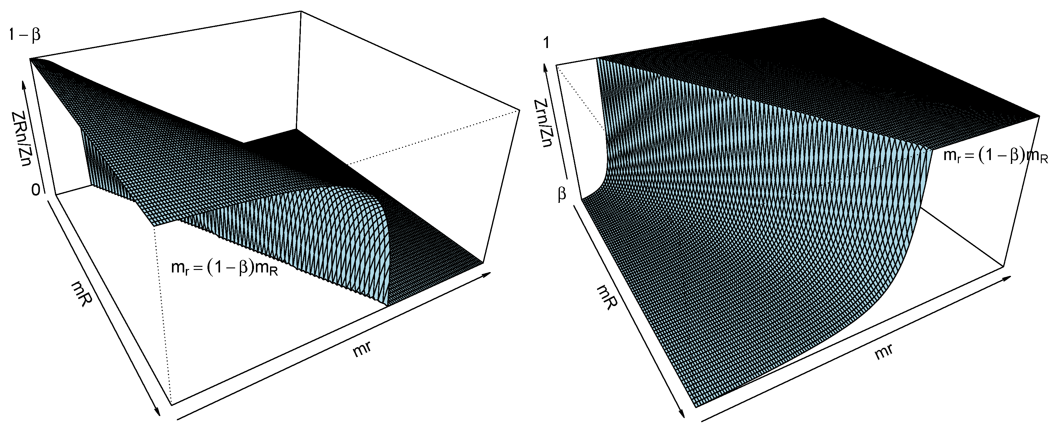
The same result can be established in termed on males. Anyway, notice that the limiting $\mathsf{R}$-genotype frequency is a constant less than or equal to $1-\beta$, achieving this maximum value when ${\mathsf{m}}_{\mathsf{r}}=0$ and the minimum (equals to 0) when ${\mathsf{m}}_{\mathsf{r}}\ge (1-\beta ){\mathsf{m}}_{\mathsf{R}}$. Hence, for the $\mathsf{r}$-genotype, the limiting frequency is always positive, higher than or equal to $\beta$, achieving this minimum value when ${\mathsf{m}}_{\mathsf{r}}=0$ and the maximum (equals to 1) when ${\mathsf{m}}_{\mathsf{r}}\ge (1-\beta ){\mathsf{m}}_{\mathsf{R}}$ (see Figure 1). We conclude thus that, independently of the mutation rate, the higher reproduction capacity of the $\mathsf{r}$-genotype, the lower the limiting $\mathsf{R}$-genotype frequency. Moreover, there is no dominant genotype in the case ${\mathsf{m}}_{\mathsf{r}}<(1-\beta ){\mathsf{m}}_{\mathsf{R}}$, which implies an important difference in comparison with the results described in [3] for the Y-linked model without mutations, where the limiting genotype frequency is null or one. Notice that this $0-1$ duality is also obtained on $\mathsf{r}$-fixation set, that is, Theorem 5 (i) holds on $\{{\mathsf{Z}}_{\mathsf{n}}^{\mathsf{R}}\to 0,{\mathsf{Z}}_{\mathsf{n}}^{\mathsf{r}}\to \infty \}$, when $(\alpha \wedge (1-\alpha )){\mathsf{m}}_{\mathsf{r}}>1$.

Finally, we give a general result related to the limiting sex frequency. One can observe that, in all cases, the limiting sex frequency in the population only depends on the probability of an offspring to be female.

Theorem 6.

It is verified that

$$\underset{\mathsf{n}\to \infty }{lim}\frac{{\mathsf{F}}_{\mathsf{n}}}{{\mathsf{F}}_{\mathsf{n}}+{\mathsf{M}}_{\mathsf{n}}}=\alpha$$

(i) 

a.s. on $\{{\mathsf{Z}}_{\mathsf{n}}^{\mathsf{R}}\to \infty \}$, if $(\alpha \wedge (1-\alpha ))(1-\beta ){\mathsf{m}}_{\mathsf{R}}>1$, and

(ii) 

a.s. on $\{{\mathsf{Z}}_{\mathsf{n}}^{\mathsf{R}}\to 0,{\mathsf{Z}}_{\mathsf{n}}^{\mathsf{r}}\to \infty \}$, if $(\alpha \wedge (1-\alpha )){\mathsf{m}}_{\mathsf{r}}>1$.

6. Illustrative Examples

In this section, the different asymptotic behaviours for an allele of a Y-linked gene and its mutations obtained in the previous sections are illustrated by means of a series of simulated examples. First, we justify the values of the parameters chosen in the simulations that follow. The sex ratio is well-known not to be balanced but closed to 0.5, being less that 0.5 in some situations (see for example [10,11]) and greater than 0.5 in others (see [12,13,14]). We fix $\alpha =0.45$, since the case $\alpha <0.5$ is mathematically more interesting. For the mutation rate, we take $\beta$ equal to $0.01$. Although such value seems to be inflated related to actual values in nature as can be seen in [15], we consider that is adequate for the convenience of modelling the process. Moreover, with respect to the number of mating units at initial generation, we consider ${\mathsf{Z}}_{\mathsf{0}}^{\mathsf{R}}=1$, which could represent Y-chromosomal most recent common ancestor with the nonmutant original allele $\mathsf{R}$ (see for example [16,17,18]), and ${\mathsf{Z}}_{\mathsf{0}}^{\mathsf{r}}=0$, since mutations appear randomly along time. Finally, Poisson distributions are considered as reproduction laws. This type of distribution is frequently used as offspring distribution (see for example [19,20,21,22,23,24]). The reproduction mean for $\mathsf{R}$-genotype is fixed taking a value of ${\mathsf{m}}_{\mathsf{R}}=2.3$ which is included in usual ranges for mammalian, for example in human (see the web page https://datos.bancomundial.org/indicador/SP.DYN.TFRT.IN). Those parameters verified that $\alpha <0.5$ and $\alpha (1-\beta ){\mathsf{m}}_{\mathsf{R}}>1$, and then there exists a positive probability of coexistence of both genotypes. In order to illustrate the different behaviours on this event, we consider the following three specific and real scenarios depending on ${\mathsf{m}}_{\mathsf{r}}$:

• In the first scenario, we consider ${\mathsf{m}}_{\mathsf{r}}=0$, that is, the $\mathsf{r}$-allele does not reproduce and, then, only appears in the population from $\mathsf{R}$-mating units via mutation. This is the case of infertility in humans, where most of the cases turn out from new random deletions on the Y chromosome in the azoospermia factor regions in an affected individual’s father who is not himself infertile (see [25] and the web page https://medlineplus.gov/genetics/condition/y-chromosome-infertility/). Notice that in this scenario, ${\mathsf{m}}_{\mathsf{r}}<(1-\beta ){\mathsf{m}}_{\mathsf{R}}$.
• On the other hand, in the next two scenarios, we consider that ${\mathsf{m}}_{\mathsf{r}}\ne 0$, and then the $\mathsf{r}$-allele may be transmitted by both types of mating units.

  –

  In the second scenario, we consider that accumulated mutations do not affect the reproductive capacity of $\mathsf{r}$-mating units, and therefore ${\mathsf{m}}_{\mathsf{r}}={\mathsf{m}}_{\mathsf{R}}$. This situation happens, for example, when the diversity of species is generated by accumulated mutations and not via natural selection (see [26,27]). Notice that in this scenario, ${\mathsf{m}}_{\mathsf{r}}>(1-\beta ){\mathsf{m}}_{\mathsf{R}}$.

  –

  In the third scenario, mutations of mutations are considered deleterious, since accumulated mutations may drive to degeneration of Y chromosome (see [28,29,30,31]). Hence, only first mutations (may be different in every stance) of males stemming from $\mathsf{R}$-type mating units are archived as $\mathsf{r}$-allele and are transmitted to descendant. Notice that in this scenario it is reasonable to assume that ${\mathsf{m}}_{\mathsf{r}}=(1-\beta ){\mathsf{m}}_{\mathsf{R}}$ by considering that couples with males stemming from a first mutation of the $\mathsf{R}$-allele have the same capacity of producing nonmutant males as an $\mathsf{R}$-couple and therefore $(1-\alpha ){\mathsf{m}}_{\mathsf{r}}=(1-\alpha )(1-\beta ){\mathsf{m}}_{\mathsf{R}}$.

In all three scenarios we simulated 20 paths of the process ${\left\{({\mathsf{Z}}_{\mathsf{n}}^{\mathsf{R}},{\mathsf{Z}}_{\mathsf{n}}^{\mathsf{r}})\right\}}_{\mathsf{n}\ge 0}$ in which both genotypes have survived until generation 500. Figure 2 illustrates the limiting genotype frequency of $\mathsf{r}$-allele, being equal to $\beta$ for the first scenario and equal to one for last two scenarios. Then, we conclude that infertile males (first scenario) are present in male population as a proportion given by the mutation rate (see [32]). On the other hand, the original nonmutant allele is negligible with respect to the mutant allele in the other two scenarios. This statement is a mathematical explanation of the evolution and diversity of species without natural selection (see [26]) and the beginning of degeneration of Y chromosome (see [33]), where nonmutant original allele disappears along time.

In the second scenario we also studied the relation between the limiting random variables ${\mathsf{W}}_{\mathsf{R}}$, ${\mathsf{W}}_{\mathsf{r}}^{*}$, and ${\tilde{\mathsf{W}}}_{\mathsf{r}}$. As previously, we considered the process starting with $({\mathsf{Z}}_{\mathsf{0}}^{\mathsf{R}},{\mathsf{Z}}_{\mathsf{0}}^{\mathsf{r}})=(1,0)$ couples and a parameter vector $(\alpha ,\beta ,{\mathsf{m}}_{\mathsf{R}},{\mathsf{m}}_{\mathsf{r}})$ with values $(0.45,0.01,2.3,2.3)$. To approximate the joint probability distribution of the random vector $({\mathsf{W}}_{\mathsf{r}}^{*},{\mathsf{W}}_{\mathsf{R}})$ we simulated 2000 paths of the process until generation 500 belonging to the coexistence set (i.e., both alleles were alive in the last observed generation). The distribution of the random vector of $({\mathsf{Z}}_{\mathsf{500}}^{\mathsf{r}},{\mathsf{Z}}_{\mathsf{500}}^{\mathsf{R}})$ with each coordinate normalised by the corresponding growth rate (to the 500th power) is considered a good enough approximation of the distribution of $({\mathsf{W}}_{\mathsf{r}}^{*},{\mathsf{W}}_{\mathsf{R}})$. Figure 3, left and middle graphs, shows the estimates of the joint distribution of $({\mathsf{W}}_{\mathsf{r}}^{*},{\mathsf{W}}_{\mathsf{R}})$ and its marginal densities, respectively, obtained using kernel density estimators, as well as the mean values of those distributions, $(12.178,14.963)$. We obtain a positive correlation between both random variables (Pearson’s correlation coefficient 0.664, p-value $<2.2\times {10}^{-16}$) and a statistically significant difference between their means (paired t-Student test: p-value $<2.2\times {10}^{-16}$). To estimate the distribution of ${\tilde{\mathsf{W}}}_{\mathsf{r}}$, we simulated again 2000 paths of the process until generation 500 but now belonging to the $\mathsf{r}$-fixation set (i.e., such that ${\mathsf{Z}}_{\mathsf{500}}^{\mathsf{R}}=0$ and ${\mathsf{Z}}_{\mathsf{500}}^{\mathsf{r}}>0$). Figure 3 (right) compares the kernel density estimates of the distributions of ${\tilde{\mathsf{W}}}_{\mathsf{r}}$ (dashed line) and ${\mathsf{W}}_{\mathsf{r}}^{*}$ (solid line) as well as their mean values ($E\left[{\tilde{\mathsf{W}}}_{\mathsf{r}}\right]\approx 7.597$ and $E\left[{\mathsf{W}}_{\mathsf{r}}^{*}\right]\approx 12.178$). In this case we also found statistically significant differences between the mean values of both distributions (Welch’s test: p-value $<2.2\times {10}^{-16}$).

7. Concluding Remarks

This work deals with the problem of determining the limiting growth rates and the limiting genotype frequencies of two alleles named $\mathsf{R}$ and $\mathsf{r}$ of a Y-linked gene, allowing the possibility that the $\mathsf{R}$-allele mutates into the $\mathsf{r}$-form assuming a two-sex (male-female) population. Moreover, the limiting sex ratio of this population is also obtained. The model studied in this communication is the so-called Y-linked bisexual branching processes with mutations and blind choice of males defined in [5]. This model studies the evolution of the number of carriers of two alleles in a two-sex monogamous population under the assumption that the considered gene has no effect on the mating process and also considering the possibility that one of the allelic forms of the gene can mutate into the other form without allowing the possibility of reversion.

We derived the limiting growth rates of surviving genotypes as functions of the mean numbers of females and males generated by a couple and the mutation rate. In particular, on the $\mathsf{r}$-fixation set such genotype evolves as a two-sex Galton–Watson branching process and therefore there exists a positive probability of survival of this genotype if the mean number of female and male offspring per $\mathsf{r}$-couple are both greater than unity. In this case, the numbers of couples and males grow geometrically at the same growth rate which is given by the mean number of females (if the probability $\alpha$ for an offspring to be female is less than or equal to 0.5) or males (if $\alpha >0.5$) per $\mathsf{r}$-couple (that is, $\alpha {\mathsf{m}}_{\mathsf{r}}$ and $(1-\alpha ){\mathsf{m}}_{\mathsf{r}}$, respectively).

On the coexistence set, both, $\mathsf{R}$ and $\mathsf{r}$-genotypes have a positive probability of survival if the mean number of female offspring per $\mathsf{R}$-couple who mate with $\mathsf{R}$-males and the mean number of male offspring per $\mathsf{R}$-couple are both greater than unity. Our results show in this case that, the growth rates for the number of $\mathsf{R}$-couples and males with $\mathsf{R}$-genotype coincide on the event of survival. In particular, both variables grow geometrically, and the limiting growth rate equals the mean number of female offspring per $\mathsf{R}$-couple who mate with $\mathsf{R}$-males if $\alpha \le 0.5$ (that is, $\alpha (1-\beta ){\mathsf{m}}_{\mathsf{R}}$, with $\beta$ being the probability of mutation), whereas it equals the mean number of $\mathsf{R}$-male offspring per $\mathsf{R}$-couple if $\alpha >0.5$ (that is, $(1-\alpha )(1-\beta ){\mathsf{m}}_{\mathsf{R}}$).

The growth rate for the number of couples and males of $\mathsf{r}$-genotype on the coexistence set turns out to be more complicated due to the mutations and it is necessary to take into account the relation between the mean number of offspring per $\mathsf{r}$-couple, ${\mathsf{m}}_{\mathsf{r}}$, and the mean number of offspring per $\mathsf{R}$-couple, ${\mathsf{m}}_{\mathsf{R}}$, multiplied by $(1-\beta )$. Notice that both quantities appeared in the previous growth rates, for $\mathsf{r}$ and $\mathsf{R}$-allele, respectively, independently on $\alpha$. So, in the case that ${\mathsf{m}}_{\mathsf{r}}>(1-\beta ){\mathsf{m}}_{\mathsf{R}}$, the numbers of $\mathsf{r}$-couples and $\mathsf{r}$-males grow geometrically at a growth rate given by the mean number of females or males (depending on weather $\alpha \le 0.5$ or $\alpha >0.5$, respectively) per $\mathsf{r}$-couple. Notice that, this behaviour is the same as the one obtained on the $\mathsf{r}$-fixation set. On the other hand, in the case ${\mathsf{m}}_{\mathsf{r}}<(1-\beta ){\mathsf{m}}_{\mathsf{R}}$, the growth rate of the numbers of $\mathsf{r}$-couples and $\mathsf{r}$-males equals the growth rate of the $\mathsf{R}$-genotype, that is, $\alpha (1-\beta ){\mathsf{m}}_{\mathsf{R}}$ if $\alpha \le 0.5$ or $(1-\alpha )(1-\beta ){\mathsf{m}}_{\mathsf{R}}$ if $\alpha >0.5$. Finally, the case ${\mathsf{m}}_{\mathsf{r}}=(1-\beta ){\mathsf{m}}_{\mathsf{R}}$ is a boundary case in which we have proved that the number of couples and males with $\mathsf{r}$-genotype along time is normalised by the sequence $\left\{\mathsf{n}{(min\{\alpha ,(1-\alpha )\}{\mathsf{m}}_{\mathsf{r}})}^{\mathsf{n}}\right\}$.

As a consequence of such results, $\mathsf{r}$-genotype is the dominant one with limiting frequency unity on the event of coexistence if ${\mathsf{m}}_{\mathsf{r}}\ge (1-\beta ){\mathsf{m}}_{\mathsf{R}}$, while ${\mathsf{m}}_{\mathsf{r}}<(1-\beta ){\mathsf{m}}_{\mathsf{R}}$ entails a balanced situations in the sense that there is not a dominant genotype and the limiting frequencies are constants which depend on ${\mathsf{m}}_{\mathsf{R}},{\mathsf{m}}_{\mathsf{r}}$ and $\beta$. In particular, the higher the reproduction capacity of the $\mathsf{r}$-genotype, the lower the limiting $\mathsf{R}$-genotype frequency, being the maximum value given by the rate of nonmutation (that is $1-\beta$) when $\mathsf{r}$-couples do not generate any descendants (that is, ${\mathsf{m}}_{\mathsf{r}}=0$). Finally, we found that the limiting female frequency equals the probability of being female in any case, and thus it does not depend on the Y-linked gene.

From a practical point of view, these mathematical results could give a scientific answer to questions of population genetics, as for example, the evolution of infertility in males (see [25,32]), the existence of degeneration of Y chromosome (see [28,29,30,31]) or the possibility of evolution and diversity of species without natural selection (see [26,27]). In particular, we conclude that although infertility conditions not to be inherited (${\mathsf{m}}_{\mathsf{r}}=0$), the frequency of this mutation in the population is not negligible along time (see [34,35,36]), and it is given by the mutation rate, $\beta$ (this is also true when the males are not infertile, but their reproductive capacity is very small, i.e., ${\mathsf{m}}_{\mathsf{r}}=(1-\beta ){\mathsf{m}}_{\mathsf{R}}$). Another conclusion is that the original nonmutant allele is negligible in the population with respect to mutations (the dominant allele) along time, when the reproductive capacity is not affected by mutations (i.e., natural selection does not work). Hence, accumulative mutations (mutation of mutation is archived, ${\mathsf{m}}_{\mathsf{r}}={\mathsf{m}}_{\mathsf{R}}$) may explain the possibility of diversity of species without natural selection (see [26]), while deleterious mutations (mutation of mutation is not archived, ${\mathsf{m}}_{\mathsf{r}}=(1-\beta ){\mathsf{m}}_{\mathsf{R}}$) could explain the beginning of the degeneration of Y chromosome (see [33,37]). Of course, the obtained results also explain the phenomenon of evolution by natural selection, since when there is a differential reproduction (${\mathsf{m}}_{\mathsf{r}}>{\mathsf{m}}_{\mathsf{R}}$), the $\mathsf{r}$-allele is the dominant allele along time.

In conclusion, the limiting behaviour of Y-linked genes in a two-sex branching process with blind choice of males and mutations shown here turns out to be the main novelty of the present work. We note that this behaviour may be different from those obtained for other two-sex branching models in a genetic context (see, for example, [3] or [38]) and also different from those obtained in classical genetic models, in which no dominant genotype exists in the population due to the Hardy-Weinberg law. Moreover, the results of the paper are expected to be a valuable contribution to the theory of two-sex branching processes and to clarify well-known phenomena of population genetics in a mathematically rigorous way. The mathematical tools used to obtained the results of this paper also allow to solve the conjectures proposed in [39] relative to the limiting growth rates for an X-linked two-sex branching process. Such a model describes the evolution of the number of carriers of the genotypes and phenotypes defined by the alleles of an X-linked gene with two alleles when one of them is considered recessive and responsible for a serious disorder of a severe disease as could be hemophilia, Duchenne muscular dystrophy, or other genetic diseases (see [40] for background information).

References

1. Kido, T.; Lau, Y.F. Roles of the Y chromosome genes in human cancers. Asian J. Androl. 2015, 17, 373–380. [Google Scholar]
2. González, M.; Martínez, R.; Mota, M. Bisexual branching processes to model extinction conditions for Y-linked genes. J. Theor. Biol. 2009, 258, 478–488. [Google Scholar] [CrossRef] [Green Version]
3. Alsmeyer, G.; Gutiérrez, C.; Martínez, R. Limiting genotype frequencies of Y-linked genes through bisexual branching processes with blind choice. J. Theor. Biol. 2011, 275, 42–51. [Google Scholar] [CrossRef] [Green Version]
4. González, M.; Gutiérrez, C.; Martínez, R. Non-parametric Bayesian inference through MCMC method for Y-linked two-sex branching processes with blind choice. J. Stat. Comput. Simul. 2018, 88, 3565–3587. [Google Scholar] [CrossRef]
5. González, M.; Gutiérrez, C.; Martínez, R. Extinction conditions for Y-linked mutant-alleles through two-sex branching processes with blind-mating structure. J. Theor. Biol. 2012, 307, 104–116. [Google Scholar] [CrossRef] [PubMed]
6. González, M.; Gutiérrez, C.; Martínez, R. Bayesian inference in Y-linked two-sex branching processes with mutations: ABC approach. IEEE/ACM Trans. Comput. Biol. Bioinform. 2019, in press. [Google Scholar]
7. Ispány, M.; Körmendi, K.; Pap, G. Asymptotic behavior of CLS estimators for 2-type doubly symmetric critical Galton–Watson processes with immigration. Bernoulli 2014, 20, 2247–2277. [Google Scholar] [CrossRef]
8. Mode, C. Multitype Branching Processes. Theory and Applications; American Elsevier Publishing Co. Inc.: New York, NY, USA, 1971. [Google Scholar]
9. Bagley, J. On the asmptotic properties of a supercritical bisexual branching process. J. Appl. Probab. 1986, 23, 820–826. [Google Scholar] [CrossRef]
10. Fu, S.; Yan, J.; Wang, X.; Dong, J.; Chen, P.; Wang, C.; Chen, G. The audiological characteristics of a hereditary Y-linked hearing loss in a Chinese ethnic Tujia pedigree. Int. J. Pediatr. Otorhinolaryngol. 2011, 75, 202–206. [Google Scholar] [CrossRef]
11. Wang, Q.; Lu, C.; Li, N.; Rao, S.; Shi, Y.; Han, D.; Li, X.; Cao, J.; Yu, L.; Li, Q.; et al. Y-linked inheritance of non-syndromic hearing impairment in a large Chinese family. J. Med. Genet. 2011, 41, e80. [Google Scholar] [CrossRef] [Green Version]
12. Bonal, R.; Hernández, M.; Espelta, J.; Munoz, A.; Aparicio, J. Unexpected consequences of a drier world: Evidence that delay in late summer rains biases the population sex ratio of an insect. R. Soc. Open Sci. 2015, 2, 150–198. [Google Scholar] [CrossRef] [PubMed] [Green Version]
13. Ellis, S.; Franks, D.; Nattrass, S.; Cant, M.; Weiss, M.; Giles, D.; Balcomb, K.; Croft, D. Mortality risk and social network position in resident killer whales: Sex differences and the importance of resource abundance. Proc. R. Soc. B 2017, 284, e1313. [Google Scholar] [CrossRef] [PubMed]
14. Hutter, S.; Li, H.; Beisswanger, S.; De Lorenzo, D.; Stephan, W. Distinctly different sex ratios in African and European populations of Drosophila melanogaster inferred from chromosomewide single nucleotide polymorphism data. Genetics 2007, 177, 469–480. [Google Scholar] [CrossRef] [PubMed] [Green Version]
15. Helgason, A.; Einarsson, A.W.; Guðmundsdóttir, V.B.; Sigurðsson, A.; Gunnarsdóttir, E.D.; Jagadeesan, A.; Ebenesersdóttir, S.S.; Kong, A.; Stefánsson, K. The Y-chromosome point mutation rate in humans. Nat. Genet. 2015, 47, 453–457. [Google Scholar] [CrossRef]
16. Cruciani, F.; Trombetta, B.; Massaia, A.; Destro-Bisol, G.; Sellitto, D.; Scozzari, R. A Revised Root for the Human Y Chromosomal Phylogenetic Tree: The Origin of Patrilineal Diversity in Africa. Am. J. Hum. Genet. 2011, 88, 814–818. [Google Scholar] [CrossRef] [Green Version]
17. Hammer, M. A recent common ancestry for human Y chromosomes. Nature 1995, 378, 376–378. [Google Scholar] [CrossRef]
18. Thomson, R.; Pritchard, J.; Shen, P.; Oefner, P.; Feldman, M. Recent common ancestry of human Y chromosomes: Evidence from DNA sequence data. Proc. Natl. Acad. Sci. USA 2000, 97, 7360–7365. [Google Scholar] [CrossRef] [Green Version]
19. Bertoin, J.; Fontbona, J.; Martínez, S. On prolific individuals in a supercritical continuous-state branching process. J. Appl. Probab. 2008, 3, 714–726. [Google Scholar] [CrossRef]
20. Blumberg, S.; Lloyd-Smith, J. Inference of r0 and transmission heterogeneity from the size distribution of stuttering chains. PLoS Comput. Biol. 2013, 9, 1–17. [Google Scholar] [CrossRef] [Green Version]
21. Farrington, C.; Grant, A. The distribution of time to extinction in subcritical branching processes: Applications to outbreaks of infectious disease. J. Appl. Probab. 1999, 36, 771–779. [Google Scholar] [CrossRef]
22. Farrington, C.; Kanaan, M.; Gay, N. Branching process models for surveillance of infectious diseases controlled by mass vaccination. Biostatistics 2003, 4, 279–295. [Google Scholar] [CrossRef] [PubMed] [Green Version]
23. Mode, C.; Sleemam, C. Stochastic Processes in Epidemiology; World Scientific: Singapore, 2000. [Google Scholar]
24. Pakes, A. Biological applications of branching processes. In Handbook of Statistic. Stochastic Processes: Modelling and Simulation; Shanbhag, D.N., Rao, C.R., Eds.; Elsevier: Amsterdam, The Netherlands, 2003; Volume 21, pp. 693–773. [Google Scholar]
25. Sun, S.; Heitman, J. Should Y stay or should Y go: The evolution of non-recombining sex chromosomes. BioEssays 2012, 342, 938–942. [Google Scholar] [CrossRef] [PubMed] [Green Version]
26. Carlin, J. Mutations are the raw materials of evolution. Nat. Educ. Knowl. 2011, 3, 10. [Google Scholar]
27. Loewe, L.; Hill, W.G. The Population Genetics of Mutations: Good, Bad and Indifferent; The Royal Society: London, UK, 2010. [Google Scholar]
28. Charlesworth, B.; Charlesworth, D. The degeneration of Y chromosomes. Philos. Trans. R. Soc. Lond. Ser. B Biol. Sci. 2000, 355, 1563–1572. [Google Scholar] [CrossRef] [PubMed] [Green Version]
29. Charlesworth, B.; Charlesworth, D. Evolution: A New Idea about the Degeneration of Y and W Chromosomes. Curr. Biol. 2020, 30, R871–R873. [Google Scholar] [CrossRef]
30. Lenormand, T.; Fyon, F.; Sun, E.; Roze, D. Sex chromosome degeneration by regulatory evolution. Curr. Biol. 2020, 30, 3001–3006. [Google Scholar] [CrossRef]
31. Steinemann, S.; Steinemann, M. Y chromosomes: Born to be destroyed. BioEssays 2005, 27, 1076–1083. [Google Scholar] [CrossRef]
32. Gershoni, M.; Pietrokovski, S. Reduced selection and accumulation of deleterious mutations in genes exclusively expressed in men. Nat. Commun. 2014, 5, 1–10. [Google Scholar] [CrossRef] [Green Version]
33. Charlesworth, B.; Charlesworth, D. Some evolutionary consequences of deleterious mutations. Genetica 1998, 102, 3. [Google Scholar] [CrossRef]
34. Hwang, K.; Yatsenko, A.; Jorgez, C.; Mukherjee, S.; Nalam, R.; Matzuk, M.; Lamb, D. Mendelian genetics of male infertility. Ann. N. Y. Acad. Sci. 2010, 1214, E1. [Google Scholar] [CrossRef] [Green Version]
35. Irvine, D. Epidemiology and aetiology of male infertility. Hum. Reprod. 1998, 13, 33–44. [Google Scholar] [CrossRef] [PubMed] [Green Version]
36. Winters, B.; Walsh, T. The epidemiology of male infertility. Urol. Clin. 2014, 41, 195–204. [Google Scholar] [CrossRef] [PubMed]
37. Bachtrog, D. Y-chromosome evolution: Emerging insights into processes of Y-chromosome degeneration. Nat. Rev. Genet. 2013, 14, 113–124. [Google Scholar] [CrossRef] [Green Version]
38. González, M.; Hull, D.M.; Martínez, R.; Mota, M. Bisexual branching processes in a genetic context: The extinction problem for Y-linked genes. Math. Biosci. 2006, 202, 227–247. [Google Scholar] [CrossRef] [PubMed]
39. González, M.; Gutiérrez, C.; Martínez, R.; Mota, M. Extinction probability of some recessive alleles of X-linked genes in the context of two-sex branching processes. In Branching Processes and Their Applications; del Puerto, I.M., González, M., Gutiérrez, C., Martínez, R., Minuesa, C., Molina, M., Mota, M., Ramos, A., Eds.; Springer: Cham, Switzerland, 2016; Chapter 17; pp. 287–305. [Google Scholar]
40. Germain, D. General aspects of X-linked diseases. In Fabry Disease: Perspectives from 5 Years of FOS; Mehta, A., Beck, M., Sunder-Plassmann, G., Eds.; Oxford PharmaGenesis: Oxford, UK, 2006; Chapter 7. [Google Scholar]
41. Stromberg, K.R. An Introduction to Classical Real Analysis; Wadsworth, Inc.: Belmont, CA, USA, 1981. [Google Scholar]
42. Kesten, H.; Stigum, B. Limit theorem for descomposable multi-dimensional Galton-Watson processes. J. Math. Anal. Appl. 1967, 17, 309–338. [Google Scholar] [CrossRef] [Green Version]
43. Hush, D.; Scovel, C. Concentration of the hypergeometric distribution. Stat. Probab. Lett. 2005, 75, 127–132. [Google Scholar] [CrossRef]
Figure 1. Limiting genotype frequency for R -allele (left) and for r -allele (right), depending on m R and m r , for fixed β .
Mathematics 09 00131 g001
Figure 2. Plot of Z n r / Z n , for several paths on coexistence set of a process when m r < ( 1 β ) m R (left), m r > ( 1 β ) m R (middle) and m r = ( 1 β ) m R (right).
Mathematics 09 00131 g002
Figure 3. (Left) Contour plot showing the joint probability distribution of ( W r * , W R ) and its mean vector. (Middle) Comparison of the kernel density estimates of the density functions of W R (dashed line) and W r * (solid line), jointly with their mean values (vertical lines). (Right) Comparison of the kernel density estimates of the distributions of W r * (solid line) and W ˜ r (dashed line), jointly with their mean values (vertical lines).
Mathematics 09 00131 g003
Publisher’s Note: MDPI stays neutral with regard to jurisdictional claims in published maps and institutional affiliations.