Estimation for Varying Coefficient Models with Hierarchical Structure

Abstract

The varying coefficient (VC) model is a generalization of ordinary linear model, which can not only retain strong interpretability but also has the flexibility of the nonparametric model. In this paper, we investigate a VC model with hierarchical structure. A unified variable selection method for VC model is proposed, which can simultaneously select the nonzero effects and estimate the unknown coefficient functions. Meanwhile, the selected model enforces the hierarchical structure, that is, interaction terms can be selected into the model only if the corresponding main effects are in the model. The kernel method is employed to estimate the varying coefficient functions, and a combined overlapped group Lasso regularization is introduced to implement variable selection to keep the hierarchical structure. It is proved that the proposed penalty estimators have oracle properties, that is, the coefficients are estimated as well as if the true model were known in advance. Simulation studies and a real data analysis are carried out to examine the performance of the proposed method in finite sample case.

1. Introduction

The varying coefficient model [1] is defined as

$$Y=\sum _{j=1}^d{X}_j{\beta }_j\left(U\right)+\epsilon ,$$

(1)

where Y is the response variable and $(X_1,X_2,\cdots ,X_d,U)$ are its associated covariates, $\epsilon$ is the error term, and ${\beta }_j\left(U\right)$ are unknown smooth coefficient functions of observable continuous covariate U. Compared with the linear model, the predictors $X_j$$(j=1,2,\cdots ,d)$ affect the response variable Y linearly, but their coefficients are allowed to change smoothly with other covariate U. Thus, each value of U is associated with a different linear model, and it also allows one to examine the extent to which the association between response Y and covariates $X_j$ varies over covariate U (see [1,2]). In environmental data analysis [2], one objective of the study is to investigate the association between the level of the pollutants and the number of daily total hospital admissions for circulatory and respiratory problems, as well as to examine how the association varies over time, where $U=t=time$. Besides, without the model specification of parametric structure and multivariate nonparametric structure, the VC model can significantly reduce the modelling bias and avoid the “curse of dimensionality”.

As the merit of good interpretability and flexibility of the varying coefficient model, a considerable amount of literature has been published on estimation and hypothesis test of the VC model since it was initiated (see, e.g., [2,3,4,5,6]). Recently, variable selection and model detection for varying coefficient model have gained much attention, for instance Wang and Xia [7] combined the ideas of the local polynomial smoothing and Lasso (least absolute shrinkage and selection operator [8]) to estimate the coefficients and select variables simultaneously; Zhao and Xue [9] employed basis function approximations and SCAD (smoothly clipped absolute deviation [10]) penalty for the semiparametric varying coefficient partially linear model; Tang et al. [11] developed a unified variable selection approach for varying coefficient models; Li et al. [12] studied the model selection and structure specification for the generalized semi-varying coefficient models; and He et al. [13] introduced a dimensionality reduction and variable selection method for multivariate varying-coefficient models with a large number of covariates, and so on.

In many complex situations, main effects combined with interaction effects may be sufficient to characterize the relationship between the response and predictors. In social, political, and economic problems and genome-wide association studies, it is useful to identify nontrivial interactions between covariates in modeling selection results, product sales, social networks, stock market changes, and disease risk. Recent years have seen a surge of interests in interaction identification in the high dimensional setting by many researchers. For instance, Hall and Xue [14] proposed a recursive approach to identify important interactions among covariates; Niu et al. [15] proposed a forward selection based screening method for identifying interactions for ultra-high dimensional data; Kong et al. [16] suggested a two-stage interaction identification method, called the interaction pursuit via distance correlation in high dimensional multi-response regression; and Radchenko and James [17] investigated variable selection for nonlinear additive regression models with interaction structures by group regularization method. Specifically, for the high dimensional linear model with interaction terms,

$$Y=\sum _{j=1}^d{X}_j{\beta }_j+\sum _{1\le j<k\le d}{X}_j{X}_k{\varphi }_{jk}+\epsilon ,$$

(2)

some important works include but are not limited to the following: Choi et al. [18] reparameterized the coefficients for the interaction terms; Bien et al. [19] added a set of convex constraints to the Lasso to produce sparse interaction terms; Zhao et al. [20] introduced the composite absolute penalties family by defining groups with particular overlapping patterns to express the relationships between the predictors; and Lim and Hastie [21] developed a method for learning pairwise interactions via hierarchical group-Lasso regularization. A key feature of the models is its hierarchical structure, as the interaction effects are derived from the main effects, which means that the interaction terms exist only if the main terms are significant in the model. This is also referred to the marginality principal in generalized linear models [22] or the strong heredity in the analysis of designed experiments [23].

Compared to parametric model (2), the VC model with interaction terms is the direct extension to the nonparametric case, where the coefficients are unknown smoothing functions of some covariates. However, the estimation methods for model (2) cannot be directly extended to the VC model with interaction terms. Variable selection for the VC model including interaction effects is also important, since ignoring important predictors can lead to biased results, while including irrelevant predictors may lead to efficiency loss. Moreover, variable selection for the VC model with interaction terms is even more complex, since nonzero functional coefficients rather than nonzero parameters need to be identified. In this paper, we aim to develop a unified variable selection method for VC model with hierarchical structure, which not merely can identify the significant variables with nonzero functional coefficients. Moreover, the selected model keeps the hierarchical structure, that is, interaction terms can be selected into the model only if the corresponding main effects are in the model. Firstly, kernel smoothing method is employed to obtain the initial estimates of the varying coefficient functions. Secondly, the local penalized least squares estimates with overlapped group Lasso penalty are proposed to simultaneously achieve variable selection and coefficients estimation, and the estimators enforce the hierarchical structure. Thirdly, it is proved that the proposed estimators have the oracle properties, that is, the functional coefficients are estimated as well as if the true model were known in advance.

The rest of the paper is organized as follows. In Section 2, we propose the local penalized least squares estimator with group Lasso penalty, which enforces the hierarchical structure. The asymptotic properties of the estimators are investigated in Section 3. In Section 4, we conduct some simulations and the Boston housing data analysis to assess the finite sample performance of the new estimators. The conclusion and future works are discussed in Section 5. Proofs of the theorems are postponed to Appendix A.

2. Modeling and Estimation

The varying coefficient model with hierarchical structure is defined as follows,

$$Y_i=\sum _{j=1}^d{X}_{ij}{\beta }_j\left(U_i\right)+\sum _{1\le j<k\le d}{X}_{ij}{X}_{ik}{\varphi }_{jk}\left(U_i\right)+{\epsilon }_i,i=1,2,\cdots ,n,$$

(3)

where $Y_i$ is the response variable, $X_{ij},j=1,2,\cdots ,d$ are the predictive variables, $U_i$ is the index covariate, ${\epsilon }_i$ is the random error and satisfies $\mathrm{E}\left({\epsilon }_i\right|X_i,U_i)=0$, $\mathrm{Var}\left({\epsilon }_i\right|X_i,U_i)={\sigma }^2\left(U_i\right)$, ${\beta }_j\left(U_i\right)$ is the unknown smooth coefficient function, and ${\varphi }_{jk}\left(U_i\right)$ is the coefficient function associated with the interaction term $X_{ij}{X}_{ik}$. The hierarchical structure means that the interaction term $X_{ij}{X}_{ik}$ exists if and only if both $X_{ij}$ and $X_{ik}$ exist in the model, namely $\int {\varphi }_{jk}^2\left(u\right)du\ne 0$ holds if and only if both $\int {\beta }_j^2\left(u\right)du\ne 0$ and $\int {\beta }_k^2\left(u\right)du\ne 0$ hold for any $i=1,2,\cdots ,n$, $1\le j<k\le d$. The model (3) is a useful extension of the linear model with hierarchical structure (2) (see, e.g., [18,19,24,25,26,27]), which can maintain the good interpretability of parameter models and also has the flexibility of the nonparametric models.

To simplify the representation of model (3), we list the following definitions,

$$\begin{array}{ccc}\hfill & X_i={(X_{i1},X_{i2},\cdots ,X_{id})}^{\tau },Z_i={(X_{i1}{X}_{i2},\cdots ,X_{i1}{X}_{id},X_{i2}{X}_{i3},\cdots ,X_{i2}{X}_{id},\cdots ,X_{id-1}{X}_{id})}^{\tau },\hfill & \hfill \\ \hfill & \mathit{\varphi }\left(U_i\right)={({\varphi }_{12}\left(U_i\right),{\varphi }_{13}\left(U_i\right),\cdots ,{\varphi }_{1d}\left(U_i\right),{\varphi }_{23}\left(U_i\right),{\varphi }_{24}\left(U_i\right),\cdots ,{\varphi }_{2d}\left(U_i\right),\cdots ,{\varphi }_{(d-1)d}\left(U_i\right))}^{\tau },\hfill & \hfill \\ \hfill & \mathit{\beta }\left(U_i\right)={({\beta }_1\left(U_i\right),{\beta }_2\left(U_i\right),\cdots ,{\beta }_d\left(U_i\right))}^{\tau },W_i={(X_i^{\tau },Z_i^{\tau })}^{\tau },\mathit{\alpha }\left(U_i\right)={(\mathit{\beta }{\left(U_i\right)}^{\tau },\mathit{\varphi }{\left(U_i\right)}^{\tau })}^{\tau },\hfill & \hfill \\ \hfill & {\mathit{\beta }}_j={({\beta }_j\left(U_1\right),{\beta }_j\left(U_2\right),\cdots ,{\beta }_j\left(U_n\right))}^{\tau },{\mathit{\varphi }}_{jk}={({\varphi }_{jk}\left(U_1\right),{\varphi }_{jk}\left(U_2\right),\cdots ,{\varphi }_{jk}\left(U_n\right))}^{\tau },\hfill & \hfill \end{array}$$

where the superscript “$\tau$” means transposition operation. Then, model (3) can be reformulated as

$$\begin{array}{c}\hfill Y_i=W_i^{\tau }\mathit{\alpha }\left(U_i\right)+{\epsilon }_i,i=1,2,\cdots ,n.\end{array}$$

Let $\Lambda =({\mathit{\beta }}_1,{\mathit{\beta }}_2,\cdots ,{\mathit{\beta }}_d,{\mathit{\varphi }}_{12},{\mathit{\varphi }}_{13},\cdots ,{\mathit{\varphi }}_{(d-1)d})$, the support set of the important main effects be $\mathcal{M}=\{j:\parallel {\mathit{\beta }}_j\parallel >0\}$, and the support set of the important interaction effects be $\mathcal{I}=\{(j,k):\parallel {\mathit{\varphi }}_{jk}\parallel >0,j,k\in \mathcal{M}\}$, where $\parallel ·\parallel$ is the $L_2$ norm.

To obtain the initial estimate of coefficient matrix $\Lambda$, we minimize the following objective function,

$$Q(\Lambda )=\sum _{t=1}^n\sum _{i=1}^n{\left[Y_i-W_i^{\tau }\mathit{\alpha }\left(U_t\right)\right]}^2{K}_h(U_t-U_i),$$

(4)

where $K_h(·)=\frac{1}{h}K(·/h)$, and $K(·)$ is a kernel function which satisfies the Condition C5 and $h\to 0$ is the bandwidth. Denote the solution to the objective function (4) by $\tilde{\Lambda }$, the tth row of $\tilde{\Lambda }$ for $t=1,2,\cdots ,n$ has the closed form

$$\tilde{\mathit{\alpha }}\left(U_t\right)={\left[\frac{1}{n}\sum _{i=1}^n{W}_i{W}_i^{\tau }{K}_h(U_t-U_i)\right]}^{-1}\left[\frac{1}{n}\sum _{i=1}^n{W}_i{Y}_i{K}_h(U_t-U_i)\right].$$

Corresponding to the assumption, only the columns of $\Lambda$ indexed by the support sets $\mathcal{M}$ and $\mathcal{I}$ are nonzero, so the main task of variable selection is to identify the sparse columns of $\Lambda$ efficiently. Meanwhile, to maintain the hierarchical structure of the model, we apply the idea of group Lasso proposed by Yuan and Lin [28] and give the following local penalized least squares estimation,

$$\begin{array}{ccc}\hfill {\widehat{\Lambda }}_{\lambda }=arg\underset{\Lambda }{min}{Q}_{\lambda }(\Lambda )& =& arg\underset{{\mathit{\beta }}_j,{\mathit{\varphi }}_{jk},1\le j<k\le d}{min}\left\{\sum _{t=1}^n\sum _{i=1}^n{\left[Y_i-W_i^{\tau }\mathit{\alpha }\left(U_t\right)\right]}^2{K}_h(U_t-U_i)\right.\hfill \\ & +& \left.\sum _{j=1}^d\left({\lambda }_j^1\sqrt{\parallel {\mathit{\beta }}_j{\parallel }^2+\sum _{k:k\ne j}^{}{\parallel {\mathit{\varphi }}_{jk}\parallel }^2}+\sum _{k:j<k}{\lambda }_{jk}^2\parallel {\mathit{\varphi }}_{jk}\parallel \right)\right\},\hfill \end{array}$$

(5)

where we assume ${\mathit{\varphi }}_{jk}={\mathit{\varphi }}_{kj}$, which is commonly used in the model with hierarchical structure, and the assumption means the interaction effects are independent of the order of the both covariates, which also significantly reduces the computation burden by lessening the number of the functional coefficients from the order of $O\left(d^2\right)$ to $O(d^2/2)$ (see [18,19,25,27]). ${\lambda }_j^1$ and ${\lambda }_{jk}^2$ are tuning parameters. For simplicity of calculations, we use the local quadratic approximation (see [10,29,30]) in each step of the iteration. Take $\tilde{\Lambda }$ as the initial estimator, which is ${\widehat{\Lambda }}_{\lambda }^{\left(0\right)}=\tilde{\Lambda }$, and, for the $(m+1)$th step, the objective function can be approximately represented as follows,

$$\begin{array}{cc}\hfill Q_{\lambda }^{(m+1)}(\Lambda )\approx & \sum _{t=1}^n\sum _{i=1}^n{\{Y_i-W_i^{\tau }\mathit{\alpha }\left(U_t\right)\}}^2{K}_h(U_t-U_i)\hfill \\ \hfill & +\sum _{j=1}^d\left({\lambda }_j^1\frac{\parallel {\mathit{\beta }}_j{\parallel }^2+{\sum }_{k:k\ne j}^{}{\parallel {\mathit{\varphi }}_{jk}\parallel }^2}{\sqrt{\parallel {\widehat{\mathit{\beta }}}_j^{\left(m\right)}{\parallel }^2+{\sum }_{k:k\ne j}^{}{\parallel {\widehat{\mathit{\varphi }}}_{jk}^{\left(m\right)}\parallel }^2}}+\sum _{k:j<k}^{}{\lambda }_{jk}^2\frac{\parallel {\mathit{\varphi }}_{jk}{\parallel }^2}{\parallel {\widehat{\mathit{\varphi }}}_{jk}^{\left(m\right)}\parallel }\right)\hfill \\ \hfill =& \sum _{t=1}^n\left\{\sum _{i=1}^n{\{Y_i-W_i^{\tau }\mathit{\alpha }\left(U_t\right)\}}^2{K}_h(U_t-U_i)\right.\hfill \\ \hfill & \left.+\sum _{j=1}^d\left({\lambda }_j^1\frac{{\beta }_j^2\left(U_t\right)+{\sum }_{k:k\ne j}^{}{\varphi }_{jk}^2\left(U_t\right)}{\sqrt{\parallel {\widehat{\mathit{\beta }}}_j^{\left(m\right)}{\parallel }^2+{\sum }_{k:k\ne j}^{}{\parallel {\widehat{\mathit{\varphi }}}_{jk}^{\left(m\right)}\parallel }^2}}+\sum _{k:j<k}^{}{\lambda }_{jk}^2\frac{{\varphi }_{jk}^2\left(U_t\right)}{\parallel {\widehat{\mathit{\varphi }}}_{jk}^{\left(m\right)}\parallel }\right)\right\}.\hfill \end{array}$$

(6)

By minimizing $Q_{\lambda }^{(m+1)}(\Lambda )$, we have

$$\begin{array}{c}\hfill {\widehat{\mathit{\alpha }}}_{\lambda }{\left(U_t\right)}^{(m+1)}={\left[\sum _{i=1}^n{W}_i{W}_i^{\tau }{K}_h(U_t-U_i)+G^{\left(m\right)}+H^{\left(m\right)}\right]}^{-1}\left[\sum _{i=1}^n{W}_i{Y}_i{K}_h(U_t-U_i)\right],\end{array}$$

(7)

where

$$G^{\left(m\right)}=\left(\begin{array}{ccccc}{M}_1^{\left(m\right)}& 0& 0& \cdots & 0\\ 0& I_{d-1}{\lambda }_1^1{\gamma }_1^{\left(m\right)}+M_2^{\left(m\right)}& 0& \cdots & 0\\ 0& 0& I_{d-2}{\lambda }_2^1{\gamma }_2^{\left(m\right)}+M_3^{\left(m\right)}& \cdots & 0\\ ⋮& ⋮& ⋮& \ddots & ⋮\\ 0& 0& 0& \cdots & {\lambda }_{d-1}^1{\gamma }_{d-1}^{\left(m\right)}+M_d^{\left(m\right)}\end{array}\right),$$

$$H^{\left(m\right)}=\left(\begin{array}{ccccc}{0}_{d\times d}& 0& 0& \cdots & 0\\ 0& {\lambda }_{12}^2{\zeta }_{12}^{\left(m\right)}& 0& \cdots & 0\\ 0& 0& {\lambda }_{13}^2{\zeta }_{13}^{\left(m\right)}& \cdots & 0\\ ⋮& ⋮& ⋮& \ddots & ⋮\\ 0& 0& 0& \cdots & {\lambda }_{(d-1)d}^2{\zeta }_{(d-1)d}^{\left(m\right)}\end{array}\right),$$

and $M_j^{\left(m\right)}=\mathrm{diag}({\lambda }_j^1{\gamma }_j^{\left(m\right)},{\lambda }_{j+1}^1{\gamma }_{j+1}^{\left(m\right)},\cdots ,{\lambda }_d^1{\gamma }_d^{\left(m\right)})$, ${\gamma }_j^{\left(m\right)}=\frac{1}{\sqrt{\parallel {\widehat{\mathit{\beta }}}_j^{\left(m\right)}{\parallel }^2+{\sum }_{k:k\ne j}{\parallel {\widehat{\mathit{\varphi }}}_{jk}^{\left(m\right)}\parallel }^2}}$, ${\zeta }_{jk}^{\left(m\right)}=\frac{1}{\parallel {\widehat{\mathit{\varphi }}}_{jk}^{\left(m\right)}\parallel }$, $1\le j<k\le d$.

Regard ${\widehat{\Lambda }}_{\lambda }$ as the Kernel Lasso (KLasso) estimator, and the specific implementation procedures can be arranged as follows:

(1)

Take the non-penalized estimator $\tilde{\Lambda }$ as the initial estimator ${\widehat{\Lambda }}_{\lambda }^{\left(0\right)}=\tilde{\Lambda }$.

(2)

According to the method discussed above, iterate (7) until convergence; specifically, the iteration stops when $max\left(|\parallel {\widehat{\mathit{\beta }}}_j^{(m+1)}\parallel -\parallel {\widehat{\mathit{\beta }}}_j^{\left(m\right)}\parallel |,|\parallel {\widehat{\mathit{\varphi }}}_{jk}^{(m+1)}\parallel -\parallel {\widehat{\mathit{\varphi }}}_{jk}^{\left(m\right)}\parallel |,1\le j<k\le d\right)$ is less than ${10}^{-3}$. For model sparsity, $\parallel {\widehat{\mathit{\beta }}}_j\parallel$ and $\parallel {\widehat{\mathit{\varphi }}}_{jk}\parallel$ should be set 0 when they are less than a small real value $c_r$ (in our simulation, we choose $c_r=0.5$).

(3)

Get the KLasso estimator ${\widehat{\Lambda }}_{\lambda }$.

Selection of bandwidth h and tuning parameters ${\lambda }_j^1$ and ${\lambda }_{jk}^2$ ($1\le j<k\le d$) is another important issue for VC model. There are two types of parameters to be considered; one common method to solve this problem is grid searching, such as cross validation (CV) or generalized cross validation (GCV) [31]. However, it would be too expensive in computation, thus here we choose h in the kernel estimation of coefficient functions by CV criterion. For the tuning parameters, we apply the idea of Zou and Li [32], where large coefficients should be given small penalties, while small coefficients should be given large penalties, and the tuning parameters can be chosen as

$${\lambda }_j^1=\frac{{\lambda }_0}{n^{-\frac{1}{2}}\left(\sqrt{\parallel {\tilde{\mathit{\beta }}}_j{\parallel }^2+{\sum }_{k:k\ne j}^{}{\parallel {\tilde{\mathit{\varphi }}}_{jk}\parallel }^2}\right)},{\lambda }_{jk}^2=\frac{{\lambda }_0}{n^{-\frac{1}{2}}\parallel {\tilde{\mathit{\varphi }}}_{jk}\parallel }.$$

Then, only one parameter, ${\lambda }_0$, needs to be considered, which is selected according to BIC criterion

$${\mathrm{BIC}}_{\lambda }=log\left({\mathrm{RSS}}_{\lambda }\right)+d_{\lambda }\frac{log\left(nh\right)}{nh},$$

where $d_{\lambda }$ is the number of nonzero coefficient functions determined by ${\widehat{\Lambda }}_{\lambda }$ and

$${\mathrm{RSS}}_{\lambda }=\frac{1}{n^2}\sum _{t=1}^n\sum _{i=1}^n{\{Y_i-W_i^{\tau }{\widehat{\mathit{\alpha }}}_{\lambda }\left(U_t\right)\}}^2{K}_h(U_t-U_i).$$

Then, ${\lambda }_0$ can be obtained by minimizing ${\mathrm{BIC}}_{\lambda }$.

3. Theoretical Properties

In this section, we establish asymptotic properties of the proposed estimator, including the model selection consistency and the oracle properties. First, we make some notations and list some regular conditions. Define $a_n=max\{{\lambda }_j^1,{\lambda }_{kl}^2:j\in \mathcal{M},(k,l)\in \mathcal{I}\}$, $b_n=min\{{\lambda }_j^1,{\lambda }_{kl}^2:j\in {\mathcal{M}}^c,(k,l)\in {\mathcal{I}}^c\}$. Let ${\mathbf{X}}_{\mathcal{M}}$ denote a matrix which is generated from $\mathbf{X}$ with columns indexed by $\mathcal{M}$, and ${\mathbf{Z}}_{\mathcal{I}}$ denotes a matrix which is generated from $\mathbf{Z}$ with columns indexed by $\mathcal{I}$, ${\mathbf{W}}_{\mathcal{S}}=({\mathbf{X}}_{\mathcal{M}},{\mathbf{Z}}_{\mathcal{I}})$, ${\mathbf{W}}_{{\mathcal{S}}^c}=({\mathbf{X}}_{{\mathcal{M}}^c},{\mathbf{Z}}_{{\mathcal{I}}^c})$, $\widehat{\mathcal{M}}=\{j:\parallel {\widehat{\mathit{\beta }}}_j\parallel >0\}$, $\widehat{\mathcal{I}}=\{(j,k):\parallel {\widehat{\mathit{\varphi }}}_{j,k}\parallel >0\}$, ${\widehat{\mathit{\alpha }}}_{\mathcal{S}}\left(U_t\right)={({\widehat{\mathit{\beta }}}_{\mathcal{M}}^{\tau }\left(U_t\right),{\widehat{\mathit{\varphi }}}_{\mathcal{I}}^{\tau }\left(U_t\right))}^{\tau }$, ${\widehat{\mathit{\alpha }}}_{{\mathcal{S}}^c}\left(U_t\right)={({\widehat{\mathit{\beta }}}_{{\mathcal{M}}^c}^{\tau }\left(U_t\right),{\widehat{\mathit{\varphi }}}_{{\mathcal{I}}^c}^{\tau }\left(U_t\right))}^{\tau }$. The convergence of $o_p(·)$ and $O_p(·)$ are defined, respectively, as follows, for random variables $\xi$ and $\mathit{\eta }$: $\xi =o_p\left(\mathit{\eta }\right)$ means that, for all $ϵ>0$, $P\left(\right|\xi /\mathit{\eta }|>ϵ)\to 0$ as $n\to \infty$; and $\xi =O_p\left(\mathit{\eta }\right)$ means that, for all $ϵ>0$, there exists $c>0$ such that $P\left(\right|\xi /\mathit{\eta }|>c)<ϵ$ as n is sufficiently large. The following traditional conditions (see [3]) are also needed.

C1.

For $1\le i\le n$, the covariate $X_i$ is independent of the error ${\epsilon }_i$.

C2.

The covariate $W_i$ has finite p-order moment, i.e., $E\parallel W_i{\parallel }^p<\infty$, where $p\ge 2$.

C3.

The density function of U, $f\left(U\right)$, is continuous and has second-order derivative.

C4.

$\Omega \left(U\right)=E(W_i{W}_i^{\tau }\mid U_i=U)$ has second-order derivative, while $E(\parallel W_i{\parallel }^4\mid U_i=U)$ and $E(\parallel {\epsilon }_i{\parallel }^2\mid U_i=U)$ are both bounded.

C5.

$K(·)$ is a symmetric kernel function, which satisfies $\int K\left(s\right)ds=1$, $\int s^{2}K\left(s\right)ds={\mu }_2<\infty$, $\int K^2\left(s\right)ds=\nu <\infty$, $\int s^2{K}^2\left(s\right)ds={\nu }_2<\infty$.

C6.

${\mathit{\beta }}_j\left(U\right)$ and ${\mathit{\varphi }}_{jk}\left(U\right)$ are all bounded and have second-order continuous derivatives for $j\in \mathcal{M}$ and $(j,k)\in \mathcal{I}$.

Theorem 1.

Suppose C1-C6 hold; if $h\propto n^{-\frac{1}{5}},{\left(nh\right)}^{-\frac{1}{2}}{a}_n\to 0$, ${\left(nh\right)}^{-\frac{1}{2}}{b}_n\to \infty ,$ then the following results hold:

(1) 

$P(\widehat{\mathcal{M}}=\mathcal{M})\to 1$ as $n\to \infty$

(2) 

$P(\widehat{\mathcal{I}}=\mathcal{I})\to 1$ as $n\to \infty$

Theorem 1 shows that the KLasso estimator can select the true model consistently. Then, we discuss the oracle properties of the KLasso estimator in Theorem 2.

Theorem 2.

Suppose C1-C6 hold; if $h\propto n^{-\frac{1}{5}},{\left(nh\right)}^{-\frac{1}{2}}{a}_n\to 0$, ${\left(nh\right)}^{-\frac{1}{2}}{b}_n\to \infty ,$ then we have

$$\underset{U_t\in [0,1]}{sup}\parallel {\widehat{\mathit{\alpha }}}_{\lambda ,\mathcal{S}}\left(U_t\right)-{\tilde{\mathit{\alpha }}}_{\mathcal{S}}\left(U_t\right)\parallel =o_p\left(n^{-\frac{2}{5}}\right),$$

for $1\le t\le n$.

Note that the optimal convergence rate of oracle estimator is $O_p\left(n^{-\frac{2}{5}}\right)$. We also observe that the difference of convergence rate between the KLasso estimator and the oracle estimator can be ignored over the univariate indicator set. Thus, we can conclude that the KLasso estimator shares the same asymptotic properties with the oracle estimator. Proofs of these two theorems are given in the Appendix.

4. Simulation Study and Real Data Analysis

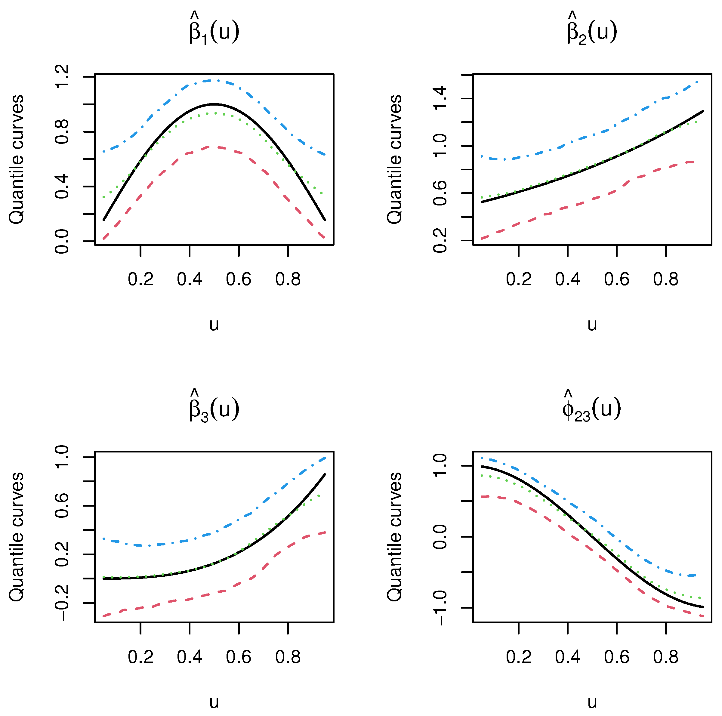
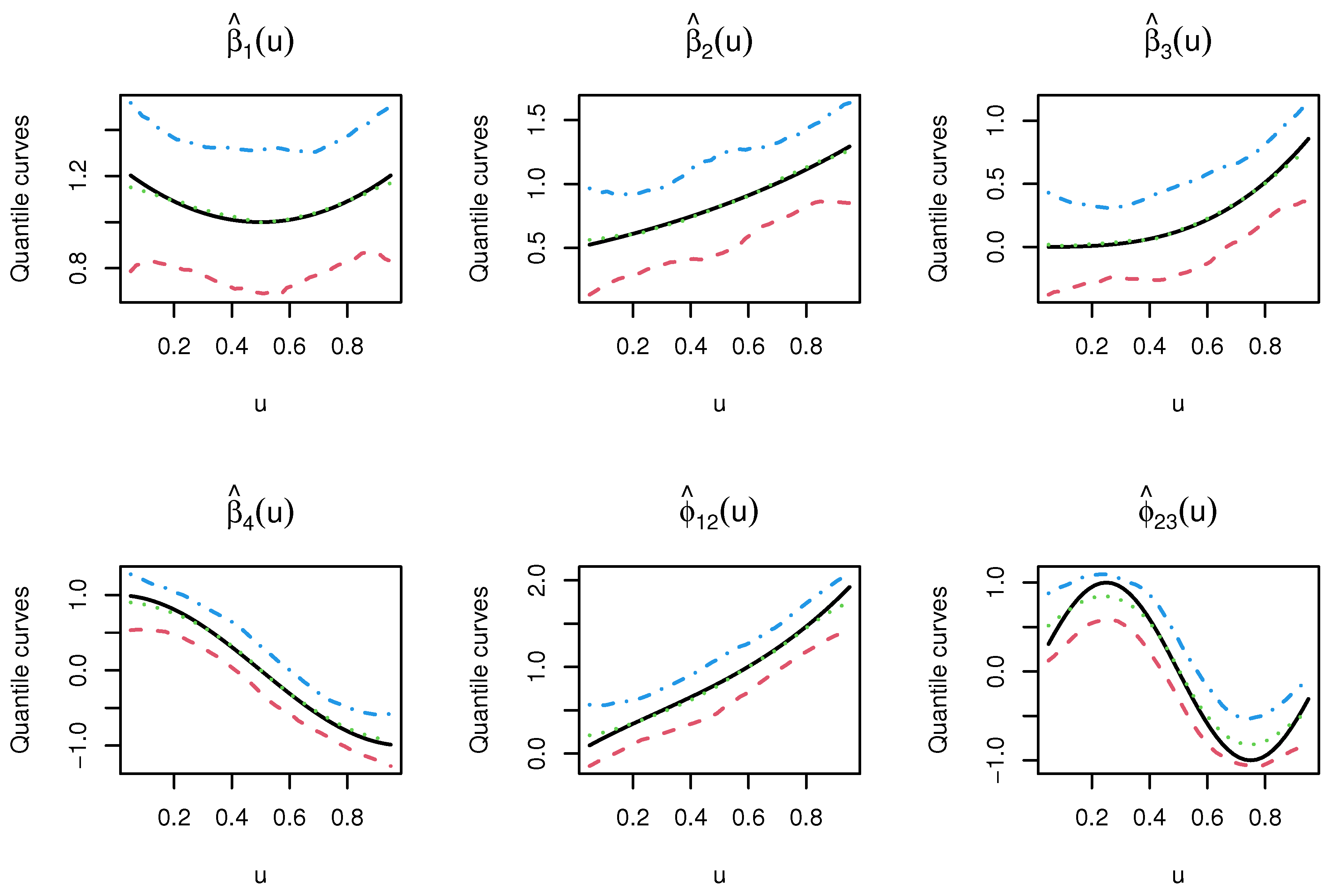
4.1. Simulation Study

In this section, three examples are applied to assess the proposed procedures in terms of varying coefficient functions estimations and variable selection. The data with sample size $n=100,200,500$ are independently generated from the following models:

$$\begin{array}{ccc}& \mathrm{Model} 1:Y_i=sin\left(\pi U_i\right)X_{i1}+0.5exp\left(U_i\right)X_{i2}+U_i^3{X}_{i3}+cos\left(\pi U_i\right)X_{i2}{X}_{i3}+{\epsilon }_i,\hfill & \hfill \\ & \mathrm{Model} 2:Y_i=[{(U_i-0.5)}^2+1]X_{i1}+0.5exp\left(U_i\right)X_{i2}+U_i^3{X}_{i3}+cos\left(\pi U_i\right)X_{i4}\hfill & \hfill \\ & +[U_i^3+log(2U_i+1)]X_{i1}{X}_{i2}+sin\left(2\pi U_i\right)X_{i2}{X}_{i3}+{\epsilon }_i,\hfill & \hfill \\ & \mathrm{Model} 3:Y_i=2U_i^2{X}_{i1}+0.5exp\left(U_i\right)X_{i2}+U^{1/3}{X}_{i3}+[cos\left(2\pi U_i\right)+cos\left(\pi U_i\right)]X_{i4}\hfill & \hfill \\ & +sin\left(2\pi U_i\right)X_{i2}{X}_{i3}+[sin\left(2\pi U_i\right)+sin\left(\pi U_i\right)]X_{i2}{X}_{i4}+{\epsilon }_i,\hfill & \hfill \end{array}$$

where the functional coefficients mainly include trigonometric function with different periods, exponential function, and power function with different locations and power. The random vector ${(X_{i1},\cdots ,X_{i10})}^{\tau }$ follows the multivariate normal distribution with zero means and $\mathrm{Cov}(X_{ij},X_{ik})=0.5^{|k-j|}$, for $1\le j<k\le 10$. The index variable $U_i\sim$Uniform[0,1] and the random error ${\epsilon }_i$ follow a standard normal distribution. In the estimation procedures, Gaussian kernel function $K\left(u\right)=\frac{1}{\sqrt{2\pi }}exp(-\frac{u^2}{2})$ is employed. The initial estimated coefficient matrix $\tilde{\Lambda }$ is obtained by minimizing (4), and the optimal bandwidth is selected via CV criterion, the selected bandwidth is also used for KLasso estimate procedure.

To assess the performance of the KLasso estimator in estimation accuracy, the empirical integrated squared error defined as follows is computed,

$$\mathrm{ISE}\left({\widehat{\beta }}_j\right)=\frac{1}{n}\sum _{i=1}^n{({\widehat{\beta }}_j\left(U_i\right)-{\beta }_j\left(U_i\right))}^2,\mathrm{ISE}\left({\widehat{\varphi }}_{jk}\right)=\frac{1}{n}\sum _{i=1}^n{({\widehat{\varphi }}_{jk}\left(U_i\right)-{\varphi }_{jk}\left(U_i\right))}^2,\mathrm{for}j\in \mathcal{M},(j,k)\in \mathcal{I}.$$

As a benchmark of comparison, the mean empirical integrated squared error (MISE) and its standard error (in parenthesis) of the oracle estimators and the proposed estimators for the three models, are respectively, reported in

Table 1. MISEs of the functional coefficients estimators for Model 1.

Estimator	$\mathit{n}=100$	$\mathit{n}=200$	$\mathit{n}=500$
${\widehat{\beta }}_1\left(u\right)$	0.0684 (0.0856)	0.0285 (0.0189)	0.0174 (0.0087)
${\widehat{\beta }}_{ora,1}\left(u\right)$	0.0553 (0.0385)	0.0277 (0.0181)	0.0170 (0.0087)
${\widehat{\beta }}_2\left(u\right)$	0.0531 (0.0508)	0.0309 (0.0213)	0.0213 (0.0110)
${\widehat{\beta }}_{ora,2}\left(u\right)$	0.0476 (0.0406)	0.0305 (0.0211)	0.0211 (0.0107)
${\widehat{\beta }}_3\left(u\right)$	0.0483 (0.0403)	0.0277 (0.0199)	0.0183 (0.0096)
${\widehat{\beta }}_{ora,3}\left(u\right)$	0.0410 (0.0325)	0.0256 (0.0167)	0.0169 (0.0086)
${\widehat{\varphi }}_{23}\left(u\right)$	0.0811 (0.0715)	0.0231 (0.0256)	0.0124 (0.0082)
${\widehat{\varphi }}_{ora,23}\left(u\right)$	0.0435 (0.0343)	0.0198 (0.0134)	0.0111 (0.0056)

,

Table 2. MISEs of the functional coefficients estimators for Model 2.

Estimator	$\mathit{n}=100$	$\mathit{n}=200$	$\mathit{n}=500$
${\widehat{\beta }}_1\left(u\right)$	0.0605 (0.0433)	0.0332 (0.0215)	0.0173 (0.0084)
${\widehat{\beta }}_{ora,1}\left(u\right)$	0.0576 (0.0407)	0.0329 (0.0212)	0.0172 (0.0083)
${\widehat{\beta }}_2\left(u\right)$	0.0832 (0.0608)	0.0428 (0.0278)	0.0221 (0.0107)
${\widehat{\beta }}_{ora,2}\left(u\right)$	0.0789 (0.0551)	0.0426 (0.0270)	0.0221 (0.0106)
${\widehat{\beta }}_3\left(u\right)$	0.0820 (0.0584)	0.0411 (0.0253)	0.0221 (0.0116)
${\widehat{\beta }}_{ora,3}\left(u\right)$	0.0753 (0.0498)	0.0419 (0.0254)	0.0225 (0.0117)
${\widehat{\beta }}_4\left(u\right)$	0.0866 (0.0882)	0.0358 (0.0323)	0.0182 (0.0095)
${\widehat{\beta }}_{ora,4}\left(u\right)$	0.0605 (0.0429)	0.0325 (0.0212)	0.0173 (0.0088)
${\widehat{\varphi }}_{12}\left(u\right)$	0.0815 (0.0685)	0.0329 (0.0213)	0.0147 (0.0081)
${\widehat{\varphi }}_{ora,12}\left(u\right)$	0.0658 (0.0486)	0.0317 (0.0202)	0.0143 (0.0077)
${\widehat{\varphi }}_{23}\left(u\right)$	0.1695 (0.1023)	0.0486 (0.0328)	0.0185 (0.0093)
${\widehat{\varphi }}_{ora,23}\left(u\right)$	0.1123 (0.0652)	0.0428 (0.0242)	0.0168 (0.0082)

and

Table 3. MISEs of the functional coefficients estimators for Model 3.

Estimator	$\mathit{n}=100$	$\mathit{n}=200$	$\mathit{n}=500$
${\widehat{\beta }}_1\left(u\right)$	0.0784 (0.0751)	0.0357 (0.0232)	0.0188 (0.0096)
${\widehat{\beta }}_{ora,1}\left(u\right)$	0.0702 (0.0536)	0.0345 (0.0224)	0.0189 (0.0096)
${\widehat{\beta }}_2\left(u\right)$	0.0938 (0.0753)	0.0483 (0.0338)	0.0253 (0.0127)
${\widehat{\beta }}_{ora,2}\left(u\right)$	0.0918 (0.0717)	0.0484 (0.0334)	0.0253 (0.0125)
${\widehat{\beta }}_3\left(u\right)$	0.0819 (0.0654)	0.0435 (0.0305)	0.0242 (0.0119)
${\widehat{\beta }}_{ora,3}\left(u\right)$	0.0795 (0.0595)	0.0435 (0.0297)	0.0244 (0.0119)
${\widehat{\beta }}_4\left(u\right)$	0.2343 (0.1158)	0.0658 (0.0385)	0.0227 (0.0113)
${\widehat{\beta }}_{ora,4}\left(u\right)$	0.2127 (0.1052)	0.0628 (0.0367)	0.0216 (0.0104)
${\widehat{\varphi }}_{23}\left(u\right)$	0.1462 (0.1213)	0.0734 (0.0660)	0.0247 (0.0126)
${\widehat{\varphi }}_{ora,23}\left(u\right)$	0.1265 (0.0897)	0.0668 (0.0483)	0.0239 (0.0118)
${\widehat{\varphi }}_{24}\left(u\right)$	0.2088 (0.1638)	0.0933 (0.0616)	0.0330 (0.0166)
${\widehat{\varphi }}_{ora,24}\left(u\right)$	0.1842 (0.1159)	0.0909 (0.0534)	0.0305 (0.0152)

. All the empirical results were computed by R software [33] based on 1000 replications. In Table 1, Table 2 and Table 3, we can see that: (1) the MISEs decrease quickly as the sample size increases for both oracle estimator and KLasso estimator; (2) the proposed estimator performs comparably well with the oracle estimator in terms of coefficients estimations for moderate sample sizes; and (3) the estimators for Model 1 have smaller MISEs compared to those of the other two models, so the number and complexity of the nonzero coefficient functions to be estimated may affect the performance of the proposed procedure in finite samples.

Let CM denote the frequency of the nonzero coefficients being correctly estimated as nonzero, CZ denote the frequency of the zero coefficients being correctly estimated as zero, and CS denote the frequency of the correctly selected model, which means that only nonzero coefficients are estimated as nonzero. CM, CZ, and CS are summarized in

Table 4. CM, CZ, and CS for Models 1–3.

	n	CM	CZ	CS
	100	0.922	0.711	0.658
Model 1	200	0.996	0.985	0.982
	500	1.000	1.000	1.000
	100	0.884	0.575	0.524
Model 2	200	0.987	0.972	0.960
	500	1.000	1.000	1.000
	100	0.932	0.533	0.517
Model 3	200	0.973	0.952	0.937
	500	1.000	1.000	1.000

. For the three models, as the sample size increases, CM, CZ, and CS all can be as large as 100%, which implies that the proposed method can identify the model well. In addition, Model 1 has the largest possibility of being correctly selected among the three models.

Besides, we also depict the quantiles curves of the estimated coefficient functions at fixed series $U_1,U_2,\cdots ,U_{46}$, where $U_i=0.05+(i-1)\times 0.02,i=1,2,\cdots ,46$. Figure 1, Figure 2 and Figure 3 are quantile curves for Models 1–3 with sample size 200, respectively. In these figures, we can see that the main effects and interaction effects can be correctly selected and consistently estimated. Meanwhile, the estimated curves usually underestimate at the peaks while overestimate at the valley of the curves. In summary, the proposed method for VC models with hierarchical structure works well.

4.2. The Boston Housing Data Analysis

To further investigate the performance of our method, we apply the proposed method to the Boston housing data which concerns the median value of owner-occupied homes (MV) for 506 census tracts in 1970. The dataset “Boston” is available in the R package “MASS” ([34]). Following the basic housing value equation of Harrison and Rubinfeld [35] and the study of Fan and Huang [3], Wang and Xia [7], we consider seven covariates here: CRIM (per capita crime rate by town), RM (average number of rooms per dwelling), NOX (nitric oxides concentration), PTRATIO (pupil-teacher ratio by town), TAX (full-value property-tax rate per $10,000), AGE (proportion of owner-occupied units built prior to 1940), and LSTAT (percentage of lower status of the population). The log transformation of MV and power transformation of RM, NOX, and LSTAT are employed to fit the Boston data well. For simplicity of representation, CRIM, RM${}^2$, TAX, NOX${}^2$, PTRATIO, and AGE are, respectively, denoted by $X_1,\cdots ,X_6$, and they are all scaled with mean zero and standard deviation 1. Meanwhile, we take $X_0\equiv 1$ as the intercept term (INT), log(MV) as the response Y, and LSTAT${}^{1/2}$ as the index variable U. Consequently, the varying coefficient model with hierarchical structure

$$Y_i={\beta }_0\left(U_i\right)+\sum _{j=1}^6{X}_{ij}{\beta }_j\left(U_i\right)+\sum _{1\le j<k\le 6}{X}_{ij}{X}_{ik}{\varphi }_{jk}\left(U_i\right)+{\epsilon }_i$$

is fitted to the Boston housing data.

The data are divided into training data and testing data with sample size 405 and 101, respectively, by sampling. Estimates are based on the training data, and performance of the proposed procedures are evaluated on the testing data. The CV criterion suggests a bandwidth $h=0.31$, and the optimal tuning parameter selected by BIC criterion is ${\widehat{\lambda }}_0=1.8$. During the implementation procedures, the variables are regarded insignificant for the mode of whose estimated functional coefficients are less than 0.1. It shows that INT, CRIM, RM${}^2$, TAX, PTRATIO, AGE, RM${}^2$×TAX are significant but the others are not. The estimated coefficient function curves for these relevant variables are depicted in Figure 4. For the testing data, compared with the VC model without considering the interaction terms, the multiple ${\mathrm{R}}^2$ for our proposed procedure is 0.8314, and it is 0.8021 without interaction terms. Thus, the proposed VC model with hierarchical structure can fit the testing data slightly better.

5. Conclusions and Future Works

In this paper, the VC models with hierarchical structure are investigated, and a unified variable selection procedure is proposed, which can simultaneously select the nonzero effects and estimate the unknown coefficient functions, while the selected model enforces the hierarchical structure. It is proved that the proposed penalty estimators have the oracle properties, that is the coefficients are estimated as well as if the true model were known in advance. Simulation studies and Boston housing data analysis are carried out to examine the performance of the proposed method in finite sample case.

However, we mainly focus on the fixed dimensionality of the predictive covariates in the paper. We will investigate the VC model with hierarchical structure in the case of diverging dimensionality of the predictors in the future. Estimation and variable selection for the generalized varying coefficient model with hierarchical structure, as well as estimation for the semiparametric varying coefficient partially linear model with hierarchical structure, are also interesting topics that deserve to be studied.

References

1. Hastie, T.; Tibshirani, R. Varying-coefficient models. J. R. Stat. Soc. Ser. B 1993, 55, 757–779. [Google Scholar] [CrossRef]
2. Fan, J.; Zhang, W. Statistical estimation in varying coefficient models. Ann. Stat. 1999, 27, 1491–1518. [Google Scholar]
3. Fan, J.; Huang, T. Profile likelihood inferences on semiparametric varying-coefficient partially linear models. Bernoulli 2005, 11, 1031–1057. [Google Scholar] [CrossRef]
4. Fan, J.; Zhang, W. Simultaneous confidence bands and hypothesis testing in varying-coefficient models. Scand. J. Stat. 2000, 27, 715–731. [Google Scholar] [CrossRef]
5. Zhu, N.H. Two-stage local Walsh average estimation of generalized varying coefficient models. Acta Math. Appl. Sin. Engl. Ser. 2015, 31, 623–642. [Google Scholar] [CrossRef]
6. Li, Z.H.; Liu, J.S.; Wu, X.L. Variable bandwidth and one step local M-estimation of varying coefficient models. Appl. Math. A J. Chin. Univ. 2009, 4, 379–390. [Google Scholar]
7. Wang, H.; Xia, Y. Shrinkage estimation of the varying coefficient model. J. Am. Stat. Assoc. 2009, 104, 747–757. [Google Scholar] [CrossRef]
8. Tibshirani, R. Regression shrinkage and selection via the lasso. J. R. Stat. Soc. Ser. B 1996, 58, 267–288. [Google Scholar] [CrossRef]
9. Zhao, P.; Xue, L. Variable selection for semiparametric varying coefficient partially linear models. Stat. Probab. Lett. 2009, 79, 2148–2157. [Google Scholar] [CrossRef]
10. Fan, J.; Li, R. Variable selection via nonconcave penalized likelihood and its oracle properties. J. Am. Stat. Assoc. 2001, 96, 1348–1360. [Google Scholar] [CrossRef]
11. Tang, Y.; Wang, H.J.; Zhu, Z.; Song, X. A unified variable selection approach for varying coefficient models. Stat. Sin. 2012, 22, 601–628. [Google Scholar] [CrossRef] [Green Version]
12. Li, D.; Ke, Y.; Zhang, W. Model selection and structure specification in ultra-high dimensional generalised semi-varying coefficient models. Ann. Stat. 2015, 43, 2676–2705. [Google Scholar] [CrossRef]
13. He, K.; Lian, H.; Ma, S.; Huang, J. Dimensionality reduction and variable selection in multivariate varying-coefficient models with a large number covariates. J. Am. Stat. Assoc. 2018, 113, 746–754. [Google Scholar] [CrossRef]
14. Hall, P.; Xue, J.H. On selecting interacting features from high-dimensional data. Comput. Stat. Data Anal. 2014, 71, 694–708. [Google Scholar] [CrossRef] [Green Version]
15. Niu, Y.S.; Hao, N.; Zhang, H.H. Interaction screening by partial correlation. Stat. Interface 2018, 11, 317–325. [Google Scholar] [CrossRef]
16. Kong, Y.; Li, D.; Fan, Y.; Lv, J. Interaction pursuit in high-dimensional multi-response regression via distance correlation. Ann. Stat. 2017, 45, 897–922. [Google Scholar] [CrossRef] [Green Version]
17. Radchenko, P.; James, G. Variable selection using adaptive nonlinear interaction structure in high dimensions. J. Am. Stat. Assoc. 2010, 105, 1541–1553. [Google Scholar] [CrossRef]
18. Choi, N.; Li, W.; Zhu, J. Variable selection with strong heredity constraint and its oracle property. J. Am. Stat. Assoc. 2010, 105, 354–364. [Google Scholar] [CrossRef]
19. Bien, J.; Taylor, J.; Tibshirani, R. A lasso for hierarchical interactions. Ann. Stat. 2013, 41, 1111–1141. [Google Scholar] [CrossRef]
20. Zhao, P.; Rocha, G.; Yu, B. The composite absolute penalties family for grouped and hierarchical variable selection. Ann. Stat. 2009, 37, 3468–3497. [Google Scholar] [CrossRef] [Green Version]
21. Lim, M.; Hastie, T. Learning interactions via hierarchical group lasso regularization. J. Comput. Graph. Stat. 2015, 24, 627–654. [Google Scholar] [CrossRef] [PubMed]
22. Nelder, J.A. The statistics of linear models: Back to basics. Stat. Comput. 1994, 4, 221–234. [Google Scholar] [CrossRef]
23. Hamada, M.; Wu, C.J. Analysis of designed experiments with complex aliasing. J. Qual. Technol. 1992, 24, 130–137. [Google Scholar] [CrossRef]
24. Haris, A.; Witten, D.; Simon, N. Convex modeling of interactions with strong heredity. J. Comput. Graph. Stat. 2016, 25, 981–1004. [Google Scholar] [CrossRef] [PubMed] [Green Version]
25. Ning, H.; Zhang, H.H. A note on high-dimensional linear regression with interactions. Am. Stat. 2017, 71, 291–297. [Google Scholar]
26. Ning, H.; Yang, F.; Zhang, H.H. Model selection for high dimensional quadratic regression via regularization. J. Am. Stat. Assoc. 2018, 113, 615–625. [Google Scholar]
27. She, Y.; Wang, Z.; Jiang, H. Group regularized estimation under structural hierarchy. J. Am. Stat. Assoc. 2018, 113, 445–454. [Google Scholar] [CrossRef]
28. Yuan, M.; Lin, Y. Model selection and estimation in regression with grouped variables. J. R. Stat. Soc. Ser. B 2006, 68, 49–67. [Google Scholar] [CrossRef]
29. Hu, T.; Xia, Y. Adaptive semi-varying coefficient model selection. Stat. Sin. 2012, 22, 575–599. [Google Scholar] [CrossRef] [Green Version]
30. Hunter, D.; Li, R. Variable selection using MM algorithms. Ann. Stat. 2005, 33, 1617–1642. [Google Scholar] [CrossRef] [Green Version]
31. Craven, P.; Wahba, G. Estimating the correct degree of smoothing by the method of generalized cross-validation. Numer. Math. 1979, 31, 377–403. [Google Scholar] [CrossRef]
32. Zou, H.; Li, R. One-step sparse estimates in nonconcave penalized likelihood models. Ann. Stat. 2008, 36, 1509–1533. [Google Scholar] [CrossRef] [PubMed]
33. R Core Team. R: A Language and Environment for Statistical Computating; R Foundation for Statistical Computing: Vienna, Austria, 2020; Available online: https://www.R-project.org/ (accessed on 16 March 2020).
34. Venables, W.; Ripley, B. Modern Applied Statistics with S, 4th ed.; Springer: New York, NY, USA, 2020; ISBN 0-387-95457-0. [Google Scholar]
35. Harrison, D. and Rubinfeld D. Hedonic housing prices and the demand for clean air. J. Environ. Econ. Manag. 1978, 5, 81–102. [Google Scholar] [CrossRef] [Green Version]
Figure 1. Estimated quantile curves of Model 1. Dash-dot lines are 0.95 quantile curves, dotted lines are 0.50 quantile curves, dashed lines are 0.05 quantile curves, and solid lines are the real function curves. The dash-dot and dashed lines indicate 90% confident bands.
Mathematics 09 00132 g001
Figure 2. Estimated quantile curves of Model 2. Dash-dot lines are 0.95 quantile curves, dotted lines are 0.50 quantile curves, dashed lines are 0.05 quantile curves, and solid lines are the real function curves. The dash-dot and dashed lines indicate 90% confident bands.
Mathematics 09 00132 g002
Figure 3. Estimated quantile curves of Model 3. Dash-dot lines are 0.95 quantile curves, dotted lines are 0.50 quantile curves, dashed lines are 0.05 quantile curves, and solid lines are the real function curves. The dash-dot and dashed lines indicate 90% confident bands.
Mathematics 09 00132 g003
Figure 4. Estimated functional coefficients curves of the relevant variables.
Mathematics 09 00132 g004