On High-Order Iterative Schemes for the Matrix pth Root Avoiding the Use of Inverses

Abstract

This paper is devoted to the approximation of matrix pth roots. We present and analyze a family of algorithms free of inverses. The method is a combination of two families of iterative methods. The first one gives an approximation of the matrix inverse. The second family computes, using the first method, an approximation of the matrix pth root. We analyze the computational cost and the convergence of this family of methods. Finally, we introduce several numerical examples in order to check the performance of this combination of schemes. We conclude that the method without inverse emerges as a good alternative since a similar numerical behavior with smaller computational cost is obtained.

1. Introduction

The computation of operators on a matrix appears in many applications. The use of iterative methods has emerged as a useful technique to approximate it. This paper is devoted to the approximation of the matrix pth root. We recall that the principal pth root of a matrix $A\in {\mathbb{C}}^{r\times r}$, where $\mathbb{C}$ is a set of complex numbers, without positive eigenvalues in $\mathbb{R}$, as the unique solution X of

$$X^p-A=0,$$

with an argument of the eigenvalues in modulus lower than

$${\displaystyle \frac{\pi }{p}}.$$

For this kind of problem, the well-known and famous Newton method takes the following form

$$X_0\mathrm{given},X_{n+1}=\frac{(p-1)X_n+A{X}_n^{1-p}}{p},n\ge 0.$$

This formula is a direct extension of the method applied to the scalar equation $x^p-a=0$. In this form, the method achieves quadratic convergence, but unfortunately, it is unstable [1]. However, as can be in seen in [2], a stable version can be found.

In fact, several applications of the Newton method exist for finding the pth root matrix, see this incomplete list of references [1,2,3,4,5,6].

Similarly, we can derive the third-order Chebyshev method as

$$X_0\in \mathrm{\Theta },X_{n+1}={\displaystyle \frac{2p^2-3p+1}{2p^2}}{X}_n+{\displaystyle \frac{2p-1}{p^2}}A{X}_n^{1-p}-{\displaystyle \frac{p-1}{2p^2}}{A}^2{X}_n^{1-2p},n\ge 0,$$

(1)

where $\mathrm{\Theta }=B\in \in {\mathbb{C}}^{r\times r}$ s.t. B has no nonpositive real eigenvalues.

In our paper [7], we proposed stable versions of this algorithm, we presented some numerical advantages of it with respect to Newton and other third-order methods such as Halley’s method [8,9], and finally, we developed a general family of any order that includes both the Newton and Chebyshev methods.

In order to develop a method avoiding the use of inverses of the different iterates, we can consider the approximation of this less natural equation $\frac{1}{x^p}-\frac{1}{a}=0$. In this case, the method presented in [7] has the form

$$\left\{\begin{array}{c}{X}_0\mathrm{given},\hfill \\ {\displaystyle X_{n+1}=X_n\sum _{k=0}^m\frac{d_k}{k!}{\left(I-A^{-1}{X}_n^p\right)}^k,n\ge 0,}\hfill \end{array}\right.$$

(2)

where

$$d_0=1\mathrm{and}{d}_k=\prod _{i=0}^{k-1}\left(\frac{1}{p}+i\right),k\ge 1.$$

This method has order m, and in particular, for $m=2$ and $m=3$, we recover the Newton and Chebyshev methods.

In the above Formula (2), we only need to compute the inverse of A. In the present paper, we propose to approximate the inverse of A by another iterative method. We can use our family introduced in [10] that has the form

$$\left\{\begin{array}{c}{Y}_0\mathrm{given},\hfill \\ {\displaystyle Y_{n+1}=\sum _{k=0}^m\left(\genfrac{}{}{0pt}{}{m+1}{k+1}\right){(-1)}^k{Y}_n{\left(A{Y}_n\right)}^k,n\ge 0.}\hfill \end{array}\right.$$

(3)

Our goal is to see that the new approach yields a similar numerical behavior but with the advantage that it is free of inverse operators, and in particular, has a smaller computational cost, which means that it requires fewer operations.

The computation of the pth root of a matrix appears, for example, in fractional differential equations, discrete representations of norms corresponding to finite element discretizations of fractional Sobolev spaces, and the computation of geodesic-midpoints in neural networks (see [11] and the references therein).

2. A General Method for Approximating the Matrix pth Root Free of Inverse Operators

As we mentioned in the introduction, for approximating $A^{\frac{1}{p}}$, we propose the use of a combination of two families. One for the approximation of $A^{-1}$ and other, that use this approximation, for the approximation of the matrix pth root.

First step: for approximating $A^{-1}$

$$\left\{\begin{array}{c}{Y}_0\mathrm{given},\hfill \\ {\displaystyle Y_{n+1}=\sum _{k=0}^m\left(\genfrac{}{}{0pt}{}{m+1}{k+1}\right){(-1)}^k{Y}_n{\left(A{Y}_n\right)}^k,n=0,\dots ,L.}\hfill \end{array}\right.$$

(4)

Second step: for approximating $A^{\frac{1}{p}}$

$$\left\{\begin{array}{c}{X}_0\mathrm{given},\hfill \\ {\displaystyle X_{n+1}=X_n\sum _{k=0}^m\frac{d_k}{k!}{\left(I-Y^L{X}_n^p\right)}^k,n\ge 0,}\hfill \end{array}\right.$$

(5)

where $Y^L$ denotes the final iteration computed by the above method (4) in the first step.

2.1. Convergence

To establish the convergence of the general method (5), we observe that

$$\begin{array}{ccc}\hfill I-A^{-1}{X}_n^p& =& I-Y^L{X}_n^p+Y^L{X}_n^p-A^{-1}{X}_n^p\hfill \\ & =& (I-Y^L{X}_n^p)+(Y^L-A^{-1})X_n^p.\hfill \end{array}$$

(6)

Now, suppose that, from method (4), we consider $n_0\in \mathbb{N}$ such that $Y_{n_0}=Y^L$. Then, for the iterative process (4), using Theorem 3.2 in [10], we obtain

$$\parallel Y^L-A^{-1}{\parallel \le \parallel A\parallel }^m\parallel Y_{n_0-1}-A^{-1}{\parallel }^{m+1}\le {\cdots \parallel A\parallel }^{{(m+1)}^{n_0}-1}{\parallel Y_0-A^{-1}\parallel }^{{(m+1)}^{n_0}}.$$

(7)

On the other hand, for the iterative process (2), from Theorem 4.1 in [7], we have

$$\parallel I-Y^L{X}_n^p\parallel <\parallel I-Y^L{X}_{n-1}^p{\parallel }^{m+1}<\cdots <{\parallel I-Y^L{X}_0^p\parallel }^{{(m+1)}^n}.$$

(8)

Finally, fixed $Y^L$ we take $X_0$ such that $\parallel I-Y^L{X}_0^p\parallel <1$. Then, from Theorem 4.1 in [7], the sequence $\left\{X_n\right\}$, given by the general method (5), converges to ${\left(Y^L\right)}^{\frac{1}{p}}$; therefore, $\left\{X_n\right\}$ is bounded. So, there exists $M>0$ such that $\parallel X_n\parallel \le M$ for all $n\in \mathbb{N}$.

Theorem 1.

Suppose $Y_0$ with $\parallel Y_0-A^{-1}\parallel <1$ and $n_0\in \mathbb{N}$ such that, from (4), we consider $Y^L=Y_{n_0}$. If $X_0$ is such that $\parallel I-Y^L{X}_0^p\parallel <1$, then for all tolerance $\mathit{Tol}>0$ given, there exists $n^{*}\in \mathbb{N}$ such that $\parallel I-A^{-1}{X}_n^p\parallel <\mathit{Tol}$ for $n⩾n^{*}$.

Proof. 

Given $\mathit{Tol}>0$, from (8), there exists $n_1\in \mathbb{N}$ such that $\parallel I-Y^L{X}_n^p\parallel <\frac{\mathit{Tol}}{2}$ for all $n⩾n_1.$

On the other hand, as $X_n$ converges to ${\left(Y^L\right)}^{\frac{1}{p}}$, from Theorem 4.1 in [7], there exists $n_2\in \mathbb{N}$ such that $\parallel {\left(Y^L\right)}^{\frac{1}{p}}-X_n\parallel <\mathit{Tol}$, for all $n⩾n_2.$ Then, $\parallel X_n\parallel \le \mathit{Tol}+\parallel {\left(Y^L\right)}^{\frac{1}{p}}\parallel$ for all $n⩾n_2.$

Moreover, from (7), given ${\displaystyle \frac{\mathit{Tol}}{2(\mathit{Tol}+\parallel {\left(Y^L\right)}^{\frac{1}{p}})}>0}$, there exists $n_3\in \mathbb{N}$ such that $\parallel Y^L-A^{-1}\parallel <\frac{\mathit{Tol}}{2}$ for all $n⩾n_3.$

Therefore, from (6), there exists $n^{*}=max\{n_1,n_2,n_3\}\in \mathbb{N}$ such that $\parallel I-A^{-1}{X}_n^p\parallel <\mathit{Tol}$ for all $n⩾n^{*}$. □

2.2. Computational Cost and Efficiency

If A is a matrix $q\times q$, and taking into account that the computational cost of the product of two matrices is $q^3$ and that adding or subtracting two matrices has a computational cost of $q^2$, then the computational cost of

• the computation of matrix $Y^L$, given by means of using (4), is $C{C}_I(m,q)=m{q}^2+(m+1)q^3$ and its computational efficiency is ${\displaystyle C{E}_I(m,q)={(m+1)}^{\frac{1}{m{q}^2+(m+1)q^3}}}$
• the computation of method (2) has a computational cost of $C{C}_R(m,q)=m{q}^2+(p+m)q^3$ and its computational efficiency is ${\displaystyle C{E}_R(m,q)={(m+1)}^{\frac{1}{m{q}^2+(p+m)q^3}}}$
• the computational cost of method (5) is obtained directly by $CC(m,q)=2m{q}^2+(p+2m+1)q^3$ and its computational efficiency is ${\displaystyle CE(m,q)={(m+1)}^{\frac{1}{2m{q}^2+(p+2m+1)q^3}}.}$

In Figure 1 and Figure 2 the computational efficiency for fixed $p=2$ and $p=3$ respectively and different values of q and m are shown.

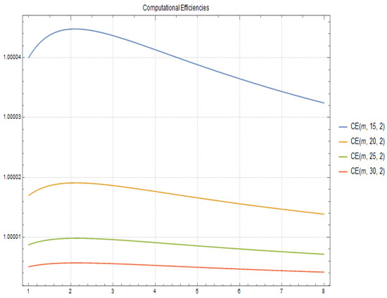
Figure 1. Computational Efficiencies for $p=2$ and different values of q and m.

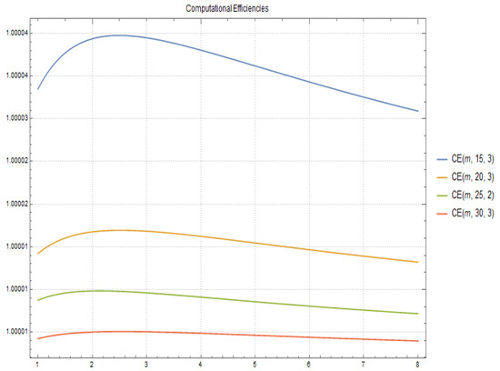
Figure 2. Computational Efficiencies for $p=2$ and different values of q and m.

In most cases, when working with a family of methods, the best one is related to the problem considered (see the next figures) and the main way used to solve the problem. For example, the most efficient method (in terms of computation) for solving sparse problems, which appear when discretizing differential equations, is Chebyshev’s method [7,10].

In Figure 3 and Figure 4 the computational efficiency for fixed $q=15$ and $q=20$ respectively and different values of p and m are shown.

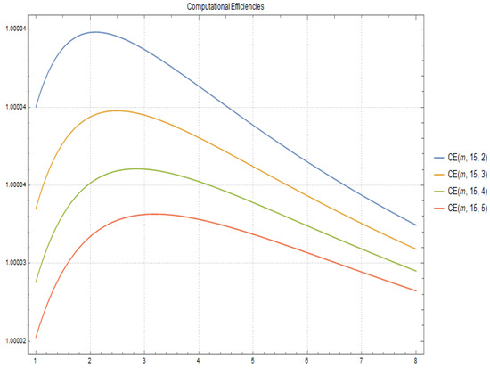
Figure 3. Computational Efficiencies for $q=15$ and different values of p and m.

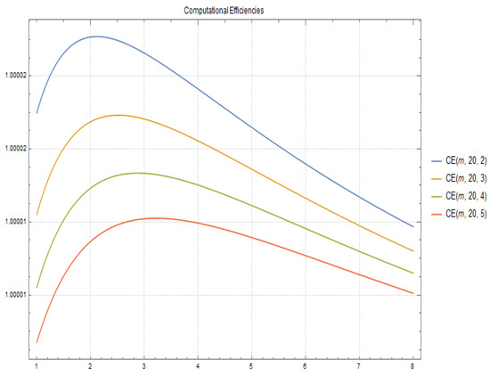
Figure 4. Computational Efficiencies for $q=20$ and different values of p and m.

3. Applications Related to Differential Equations

In this section, we present a comparison of the original method (2) using $A^{-1}$ and the new proposal (5), avoiding the use of any inverse operator. We refer to our paper [7] in order to see the advantages of the original method in comparison with other methods that appear in the literature.

We consider the approximation of the pth root of two matrices related to the discretization of differential equations. This type of matrix operations appears in the approximation of space-fractional diffusion problems [12].

We start with the following matrix

$$A=\left(\begin{array}{cccccc}C& D& & & & \\ B& C& D& & 0& \\ & B& C& D& & \\ & & \ddots & \ddots & \ddots & \\ & 0& & B& C& D\\ & & & & B& C\end{array}\right),$$

(9)

where $B=-1-\frac{h}{2}w,C=2+h^{2}v$ and $D=-1+\frac{h}{2}w$.

The matrix (9) can be seen as the result of applying a discretization process, using finite differences to the boundary value problem defined as

$$x^{″}\left(t\right)=v·x\left(t\right)+w·x^{\prime }\left(t\right),$$

where

$$x\left(a\right)=x_{a}andx\left(b\right)=x_b,$$

Since the matrix A is sparse, the most efficient methods in both families are Chebyshev-like methods.

In Table 1, we compare our original method using $A^{-1}$ (2) and the new combination using the approximation $Y^L$ of the inverse (5). We observe a similar numerical behavior of both methods. Thus, the approximation of the inverse seems a good alternative since has similar errors with smaller computational cost.

Table 1. Error for the approximation of $A^{1/p}$, taking $(m,h,v,w)=(100,0.01,$ 20,000, $-10$) and four iterations.

p	Original Method Computing ${\mathit{A}}^{-1}$	New Combined Method with Smaller Cost
2	$1.4845\times 10{}^{-11}$	$1.4845\times 10{}^{-11}$
4	$3.6643\times 10{}^{-13}$	$3.6639\times 10{}^{-13}$
6	$3.1660\times 10{}^{-13}$	$3.1655\times 10{}^{-13}$
8	$3.2326\times 10{}^{-13}$	$3.2326\times 10{}^{-13}$

Finally, we compute the pth matrix roots for the matrix

$$A=\left(\begin{array}{cccccc}1-2\lambda & \lambda & & & & \\ \lambda & 1-2\lambda & \lambda & & 0& \\ & \lambda & 1-2\lambda & \lambda & & \\ & & \ddots & \ddots & \ddots & \\ & 0& & \lambda & 1-2\lambda & \lambda \\ & & & & \lambda & 1-2\lambda \end{array}\right)$$

This matrix is related to the discretization, using finite differences, of the laplacian operator that appear in many mathematical models. In Table 2, we observe again a similar numerical behavior of both schemes.

Table 2. Error for the approximation of $A^{1/p}$ taking $m=100$, $k=2\times 10{}^{-6}$, $k/h^2=2\times 10{}^{-2}$ and three iterations.

p	Original Method Computing ${\mathit{A}}^{-1}$	New Combined Method with Smaller Cost
2	$2.1204\times 10{}^{-14}$	$2.1208\times 10{}^{-14}$
4	$1.8486\times 10{}^{-14}$	$1.8484\times 10{}^{-14}$
6	$1.7260\times 10{}^{-14}$	$1.7261\times 10{}^{-14}$
8	$2.0723\times 10{}^{-14}$	$2.0724\times 10{}^{-14}$

4. Conclusions

The function evaluation of a matrix appears in a large and growing number of applications. We have presented and studied a general family of iterative methods without using inverse operators, for the approximation of the matrix pth root. The family incorporates the approximation of $A^{-1}$, by an iterative method, into another iterative method for approximating $A^{1/p}$. The family includes methods of every order of convergence.

As it appears in [7,10], the most efficient method, in computational terms, for solving sparse problems, which appears when discretizing differential equations, is Chebyshev’s method.

Some numerical examples related to the discretization of differential equations have been presented. We have concluded that the new approach (5) has a similar numerical behavior to that of (2) but with the advantage that it is free of inverse operators, and in particular, has a lower computational cost. Finally, we care to mention the existence of other strategies for computing fractional powers of a matrix, which do not use matrix iterations [13,14] or even take into account other techniques such as those appearing in [15].

References

- Higham, N.J. Newton’s method for the matrix square root. Math. Comp. 1986, 46, 537–549. [Google Scholar]
- Iannazzo, B. On the Newton method for the matrix pth root. SIAM J. Matrix Anal. Appl. 2006, 28, 503–523. [Google Scholar] [CrossRef]
- Guo, C.-H.; Higham, N.J. A Schur-Newton method for the matrix pth root and its inverse. IAM J. Matrix Anal. Appl. 2006, 28, 788–804. [Google Scholar] [CrossRef]
- Iannazzo, B. A note on computing the matrix square root. Calcolo 2003, 40, 273–283. [Google Scholar] [CrossRef]
- Petkov, M.; Bors̆ukova, S. A modified Newton method for obtaining roots of matrices. Annu. Univ. Sofia Fac. Math. 1974, 66, 341–347. (In Bulgarian) [Google Scholar]
- Smith, M.I. A Schur algorithm for computing matrix pth roots. SIAM J. Matrix Anal. Appl. 2003, 24, 971–989. [Google Scholar] [CrossRef]
- Amat, S.; Ezquerro, J.A.; Hernández-Verón, M.A. On a new family of high-order iterative methods for the matrix pth root. Numer. Linear Algebra Appl. 2015, 22, 585–595. [Google Scholar] [CrossRef]
- Guo, C.-H. On Newton’s method and Halley’s method for the principal pth root of a matrix. Linear Algebra Appl. 2010, 432, 1905–1922. [Google Scholar] [CrossRef]
- Iannazzo, B. A family of rational iterations and its application to the computation of the matrix pth root. SIAM J. Matrix Anal. Appl. 2008, 30, 1445–1462. [Google Scholar] [CrossRef]
- Amat, S.; Ezquerro, J.A.; Hernández-Verón, M.A. Approximation of inverse operators by a new family of high-order iterative methods. Numer. Linear Algebra Appl. 2014, 21, 629–644. [Google Scholar] [CrossRef]
- Higham, N.J.; Al-Mohy, A.H. Computing Matrix Functions; The University of Manchester, MIMS EPrint: Manchester, UK, 2010; Volume 18. [Google Scholar]
- Szekeres, B.J.; Izsák, F. Finite difference approximation of space-fractional diffusion problems: The matrix transformation method. Comput. Math. Appl. 2017, 73, 261–269. [Google Scholar] [CrossRef]
- Iannazzo, B.; Manasse, C. A Schur logarithmic algorithm for fractional powers of matrices. SIAM J. Matrix Anal. Appl. 2013, 34, 794–813. [Google Scholar] [CrossRef][Green Version]
- Higham, N.J.; Lin, L. An improved Schur–Pade algorithm for fractional powers of a matrix and their Fréchet derivatives. SIAM J. Matrix Anal. Appl. 2013, 34, 1341–1360. [Google Scholar] [CrossRef]
- Marino, G.; Scardamaglia, B.; Karapinar, E. Strong convergence theorem for strict pseudo-contractions in Hilbert spaces. J. Inequalities Appl. 2016, 2016, 134. [Google Scholar] [CrossRef]
Publisher’s Note: MDPI stays neutral with regard to jurisdictional claims in published maps and institutional affiliations. |
© 2021 by the authors. Licensee MDPI, Basel, Switzerland. This article is an open access article distributed under the terms and conditions of the Creative Commons Attribution (CC BY) license (http://creativecommons.org/licenses/by/4.0/).