Detecting Jump Risk and Jump-Diffusion Model for Bitcoin Options Pricing and Hedging

Abstract

In this paper, we conduct a fast calibration in the jump-diffusion model to capture the Bitcoin price dynamics, as well as the behavior of some components affecting the price itself, such as the risk of pitfalls and its ambiguous effect on the evolution of Bitcoin’s price. In addition, in our study of the Bitcoin option pricing, we find that the inclusion of jumps in returns and volatilities are significant in the historical time series of Bitcoin prices. The benefits of incorporating these jumps flow over into option pricing, as well as adequately capture the volatility smile in option prices. To the best of our knowledge, this is the first work to analyze the phenomenon of price jump risk and to interpret Bitcoin option valuation as “exceptionally ambiguous”. Crucially, using hedging options for the Bitcoin market, we also prove some important properties: Bitcoin options follow a convex, but not strictly convex function. This property provides adequate risk assessment for convex risk measure.

1. Introduction

In the Fintech era, Bitcoin has shown remarkable performance in the decade since Nakamoto (2008) invented the cryptocurrency, due the blockchain-based and decentralized system. It has also risen rapidly in market capitalization since the COVID-19 pandemic outbreak. In the past decade, Bitcoin prices have been extremely volatile, and its abnormal return expands the potential in phases of extreme price; unpredictable and massive crashes broke out after the 2017/18 crash. Consequently, the price of Bitcoin appears to jump. As shown in Figure 1, the price of Bitcoin rose by more than 1900 percent in 2017, starting the year at around USD 1000 and grazing almost USD 20,000 in mid-December. However, there is still no clear explanation as to why there is a price jump, that is, a sudden spike in interest. Bitcoin is notoriously volatile and has seen multiple booms and crashes. As previously stated, these peaks are in line with price bubbles, and the current Bitcoin market is comparable to the internet bubble of the late 1990s. A popular ambiguity model in finance is the ambiguous volatility approach. Models with ambiguous volatility and jumps in returns and volatility are quite different to contingent claims usages which have no analytic solutions. A more effective approach was proposed by the implied diffusion approach of Poisson jumps by Dupire [1] and Andersen and Andreasen [2]. They show significant evidence that this technique exhibits some dominant in terms of capturing the form of a smile or a skew of implied volatilities. In addition, there are several studies addressing the valuation of options under jump-diffusion processes. In response, Ma et al. [3] apply in univariate and self-exciting (i.e., Hawkes) jump-diffusion models to the valuation of European-type contingent claims. Moreover, two different hedging strategies, which are used for the option under a jump-diffusion model, were explored by He et al. [4]. Briefly, there are two crucial problems when the underlying asset follows Merton [5] and Bates’ [6] jump-diffusion process. First, the calibration is an ill-posed inverse problem, even for simple jump-diffusion models, and may lead to calibration bias of model parameters that have serious effects on hedging performance and valuation of derivatives, see Cont and Tankov [7]. Second, a contingent claim cannot be hedged perfectly with standard marketed instruments available when the underlying asset returns follows a jump-diffusion with possible jump size taking values on a continuum, see, e.g., Gómez-Valle and Martínez-Rodríguez [8].

The purpose of this paper is to address the important issue that cryptocurrencies involve significant jump risks, in which they behave in a highly volatile manner, are vulnerable to hacking, and most transactions are aimed at speculative investments in Bitcoin. The volatility and speculative nature of cryptocurrencies indicates the necessity for diversification and hedging across market platforms (see Luther and White [9]). The conclusion reached so far is that Bitcoin are considered a store of value asset class or speculative investment, rather than a currency. As for the empirics of Bitcoin’s price, volatility observed in this market is a major concern, for example, Yermack [10] argued that Bitcoin prices are considerably more volatile than gold prices. In addition, Dowd and Hutchinson [11] draw a very drastic conclusion: “Bitcoin will bite the dust”. Furthermore, the preliminary findings of current works (e.g., Ardia et al. [12], Fang et al. [13], Bouri et al. [14], Bouri and Gupta [15], and Cao and Celik [16]), argue that the heightened volatility of Bitcoin prices is likely to be driven by the uncertainty macroeconomics, e.g., the US–China trade war and the COVID-19 pandemic outbreak. Recently, a few studies have been devoted to combining the Bitcoin literature with that on option pricing to construct Bitcoin option pricing models with dynamic jumps. There are several notable papers on this topic, such as Scaillet, Treccani, and Trevisan [17], Siu and Elliott [18], Jalan, Matkovskyy, and Saqib [19], which have documented the earlier analysis. However, these literatures do not provide a specific measure by detecting jumps for implied volatility in jump-diffusion models, and the option is hedged with the underlying Bitcoin.

In this paper, we focus on theoretical properties for the suggested model; the choice for the most suitable model parameters among the ones proposed in the literature is made in view of market data considering historical volatility and jumps (e.g., Hilliard et al [20]). It is worth noting that a market for these contingent claims has recently appeared in the existing literature, such as Kapetanios, Neumann, and Skiadopoulos [21] and Qiao et al. [22].

Our study makes the following contributions: From a theoretical viewpoint, it contributes to a recently emerged literature in two ways. First, the model is proven to elaborate on how Bitcoins can be captured using a fast calibration in the Bates jump-diffusion process. Second, we conduct an in-depth investigation of hedging strategies with perfect replication of a contingent claim. The paper empirically analyses the behavior of Bitcoin prices; we contribute to the literature by fitting the calibrated model combining the ambiguous parameters and detecting spurious jump component from

Table 1. Descriptive statistics on significant jumps using LM statistics.

	Q1		Q2		Q3		Q4
	No. of Jumps	P(Jump freq.)	No. of Jumps	P(Jump freq.)	No. of Jumps	P(Jump freq.)	No. of Jumps	P(Jump freq.)
2015	45	0.125	52	0.1429	61	0.1685	44	0.1196
# Observations	360		364		368		368
2016	45	0.1236	42	0.1154	47	0.1291	37	0.1016
# Observations	364		364		368		368
2017	38	0.1056	36	0.0989	50	0.1359	41	0.1114
# Observations	360		364		368		368
2018	35	0.1483
# Observations	236
# jumps	573
(Mean) (Std. dev.) (Total Obs.	(0.124)
	(0.02)
	4,620

Regarding number of jumps and jump intensity, we further provide the total number jumps (# jumps), their proportion (%) over sample observations, i.e., expressed as (P(jump) = 100(#jumps/#obs.)), and their mean and standard deviation of full sample observations (values in parentheses). Quarterly estimates for BTC and no. of jumps represents number of detected jumps, and P (jump freq.) implies the proportion of observations with a significant jump arrivals at α = 0.05. LM statistics represent the Lee and Mykland [23] jump test statistic.

.

The rest of the paper is s organized as follows. In Section 2, we briefly describe the jump detection technique to capture the Bitcoin price dynamics and calculus the intensity of the jumps. In Section 3 we introduce a quasi-closed formula for European-style options for Bitcoin derivations pricing and computation of Greeks. Section 4 is devoted to a numerical application and some preliminary results. Finally, Section 5 offers some concluding remarks. Most technical proofs are provided in the Appendix.

2. Methodology

2.1. Jump Detection Methodology

The evolution of Bitcoin prices under jump-diffusion processes can be expressed the following stochastic differential equation as:

$$d\log P_t= {\mu }_{t}dt+\sigma \left(t\right)d{W}_t+Y_{t}d{J}_t$$

(1)

where ${\mu }_t$, σ(t) and $W_t$ are the drift and volatility stochastic processes and the Brownian motion, respectively, such that $d\log P_t$ denotes an Itô process with continuous sample paths; $J_t$ is a counting process that controls the jumps arrival; and $Y_t$ represents the jump size.

Due to competing approaches, the study uses Lee and Mykland’s [23] jump detection technique to identify whether there are any arrival jumps in Bitcoin prices for a review of frequency jump detection. Moreover, the jump detection test proposed by Lee and Mykland [23] can identify jumps that occur at any time during the trading day in financial assets, whereas the other jump tests in the existing literature can merely examine the daily discontinuous sample-path, see Dumitru and Urga [24]. The discrete time returns of Equation (1) are expressed as follows:

$$R_t= \log (P_t) - \log (P_{t-1})$$

(2)

where $R_t$ is the log return. Additionally, to formally define our empirical volatility measures on the trading day t, we sum the squared j-th intraday returns by:

$$R{V}_t={\displaystyle \sum }_{j=1}^M{R}_{t,j}^2$$

(3)

where M refers to the number of observations within the measurement time frame. Multiply the above estimator by π/2, a consistent estimator for quadratic variance in the arrival jumps, to obtain the realized bipower variation (BV) as follows:

$$B{V}_t\equiv \frac{\pi }{2}\frac{M}{M-1}{\displaystyle \sum }_{j=2}^M\left|R_{t,j}\right|\left|R_{t,j-1}\right|$$

(4)

where the $\frac{M}{M-1}$ term indicates a finite sample correction. Therefore, an empirically more robust measure was developed by Huang and Tauchen [25] as the following relative jump statistic, defined as:

$$R{J}_t=\frac{R{V}_t-B{V}_t}{R{V}_t}$$

(5)

or the corresponding (approximate) logarithmic form can be expressed as:

$$R{J}_t\equiv \log R{V}_t-\log B{V}_t$$

(6)

In addition, both $B{V}_t$ and $R{J}_t$, in order to capture the distinct components, are calculated for the total daily price variation. Therefore, the jump detection statistic is defined as:

$$ℒ\left(i\right)=\frac{R_{t,i}}{\widehat{{\sigma }_{t,i}}}$$

(7)

where ${\widehat{{\sigma }_{t,i}}}^2$ = $\frac{1}{K-2}{\sum }_{j=i-K+2}^{i-1}\left|R_{t,j}\right|\left|R_{t,j-1}\right|$, and K is the window size. Additionally, Lee and Mykland [23] construct a rejection region to test the null hypothesis of no jump at $\left(t_{i-1},t_i\right]$ at a given significance level $\alpha$ meeting the following condition:

$$\frac{\left|ℒ\left(i\right)\right|-C_n}{S_n}>-\log \left(-\log \left(1-\alpha \right)\right)$$

(8)

where $C_n=\frac{\sqrt{2\log n}}{0.7979}-\frac{\log \pi +\log \left(\log n\right)}{1.5958\sqrt{2\log n}}$,$S_n=\frac{1}{1.5958\sqrt{2\log n}}$. The null hypothesis of no jumps is rejected whenever $\frac{ℒ\left(i\right)- C_n}{S_n}$>$\beta$* exceeds the critical value $\beta$* under a significance level of $\alpha$= 0.05. For a given confidence level 𝛼 is obtained with $\beta$* such that exp(—$e^{-{\beta }^{*}}$) = $1-\alpha$ = 0.95, namely, $\beta$*$=-\log \left(-\log \left(0.95\right)\right)=2.9702$. This procedure can be expected to detect only a spurious jump in a given sample of n observations. Finally, by the above procedure, we can obtain the jump intensity, and these results can later be applied as a setting parameter to calibrate in the Bates model.

2.2. The Bitcoin and Its Options Market Model

To model uncertainty, we consider a complete, filtered, probability space $\left(\Omega ,ℱ, \mathbb{P}\right)$ with a right-continuous filtration ${\left({ℱ}_{\mathrm{t}}\right)}_{\mathrm{t}>0}$ that satisfies the usual conditions of completeness on which is defined the price process $S$ = ${\left(S_t\right)}_t$ of a Bitcoin asset. This asset serves us later as underlying European derivatives. Using Ito’s Lemma, the corresponding model for the Bitcoin price under the physical probability measure $\mathbb{P}$, the Bitcoin price whose return dynamics are given by the following:

$$\frac{d{S}_t}{S_t}=\left(\mu -\lambda \overline{k}\right)dt+\sigma W_t+kd{N}_t$$

(9)

where $\mu$,σ are the instantaneous expected return and the instantaneous volatility, respectively, scaled to correspond to the unit time interval; $W_t$ denotes a standard Wiener process under the market measure $\mathbb{P}$. The $N_t$ follows a Poisson counting process, with the mean number of jumps per unit time $\lambda$ under the measure $\mathbb{P}$ so that arrival jump intensity is also given by:

$$d{N}_t=\{\begin{array}{l}0 \mathrm{with} \mathrm{probability} 1-\lambda dt,\\ 1 \mathrm{with} \mathrm{probability} \lambda dt.\end{array}$$

(10)

where $k$ is magnitude of the sudden jumps, the expected proportional jump size takes the form:

$$\overline{k}\equiv {\mathbb{E}}_{\mathbb{P}}\left(e^J-1\right).$$

We next extend the jump-diffusion model and obtain a diffusion approximation as the following right-continuous process, also called the Levy–Itô decomposition:

$$S_t=S_0+\left[b-\lambda \overline{k}\right] t+\sigma W_{}^Q\left(t\right)+k{\displaystyle \sum }_{i=1}^{N\left(t\right)}{J}_i$$

(11)

where $S_0$ is the initial price level of Bitcoin and $b$ is cost-of-carry for Bitcoin options. Their price dynamics follow the stochastic differential equation described by:

$$\frac{d{S}_t}{S_t}=\left(b-\lambda \overline{k}\right)t+\sigma W_{}^Q\left(t\right)+\left(J_i-1\right)dNt$$

(12)

Suppose ${\mathbb{Z}}_t$ is a jump-diffusion process with evolution given by:

$${\mathbb{Z}}_t={\mathbb{Z}}_0+{\int }_0^t{a}_s d_s+{\int }_0^t\sigma dW+{\sum }_{i=1}^{N_t}\Delta {\mathbb{Z}}_i$$

(13)

where $a_s$ is the drift term, $\sigma$ is the volatility term, and $\Delta {\mathbb{Z}}_i$ corresponds to jump i in the Bitcoin price. Then, using Ito’s formula for jump-diffusions, the stochastic equation can be further obtained as follows:

$$ln{S}_t=ln{S}_0+\left[b-\lambda \overline{k}-\frac{{\sigma }^2}{2}\right]\left(t\right)+\sigma W_t+{\displaystyle \sum }_{i=1}^{Nt}ln{J}_i$$

(14)

We next obtain the following after taking the exponential of the previous equation

$$S_t=S_0\exp \left\{\left(b-\frac{{\sigma }^2}{2}\right)t+\sigma W_t\right\}\exp \left({\displaystyle \sum }_{i=1}^{Nt}ln{j}_i\right)$$

(15)

It is worth recalling the assumption that the price fluctuation of Bitcoin follows a log-normal diffusion process with jumps. Specifically, using the previous definition of the price log-return jump size, that is $ln{j}_i\equiv J_i$. Then, for a given under jump-diffusion, the corresponding Bitcoin price fluctuations process $S_t$ satisfies the stochastic equation

$$S_t=S_{0}exp\left[\left(b-\frac{{\sigma }^2}{2}\right)t+\sigma W_t\right]\left({\displaystyle \prod }_{i=1}^{N_t}{J}_i\right)$$

(16)

2.3. Fourier Transform and Moments of Bitcoin’s Returns Dynamic

From the above model, several interesting implicit parameters, such as implied total annual volatility, can also be found. When the underlying process under $\mathbb{P}$ is defined by Equation (9), then the log return process is given by:

$$\begin{gathered} Ln\frac{S_t}{S_0}=\left[\left(\alpha -\frac{1}{2}{\sigma }^2-\lambda \overline{k}\right)t+\sigma W_t+{\displaystyle \sum }_{i=1}^{N_t}ln\left(j_i\right)\right] \\ =\left[\left(\alpha -\frac{1}{2}{\sigma }^2-\lambda \overline{k}\right)t+\sigma W_t+{\sum }_{i=1}^{N_t}ln\left(j_i\right)\right] \end{gathered}$$

(17)

The characteristic function of the Bitcoin’s log-return process can be expressed as the following expectation by using the Fourier transform of the log-return density function.

$$\begin{array}{l}{ℱ}_{\omega }\left(ln\frac{S_t}{S_0}\right)=E\left[exp\left(i\omega ln\frac{S_t}{S_0}\right)\right]\\ =E\left[exp\left(i\omega \left(\alpha -\frac{1}{2}{\sigma }^2-\lambda \overline{k}\right)t\right)\right]E\left[exp\left(i\omega \sigma W_t\right)\right]E\left[exp\left({\sum }_{i=1}^{N_t}i\omega J_i \right)\right]\\ =exp\left[i\omega \left(\alpha -\frac{1}{2}{\sigma }^2-\lambda \overline{k}\right)t\right]exp\left[\frac{1}{2}{\left(i\omega \sigma \right)}^{2}t\right]E\left[exp\left({\sum }_{i=1}^{N_t}i\omega ln(j_i) \right)\right]\\ =exp\left[i\omega \left(\alpha -\frac{1}{2}{\sigma }^2-\lambda \overline{k}\right)t-\frac{1}{2}{\left(\omega \sigma \right)}^{2}t\right] \left[exp\left(\lambda tE\left(j_{}^{i\omega }-1\right) \right)\right]\\ =exp\left[i\omega \alpha t-\frac{1}{2}i\omega {\sigma }^{2}t-i\omega \lambda \overline{k}t-\frac{1}{2}{\omega }^2{\sigma }^{2}t+\lambda tE\left(j_{}^{i\omega }-1\right)\right] \\ {ℱ}_{\omega }\left(ln\frac{S_t}{S_0}\right)=exp\left\{i\omega \alpha t-\frac{1}{2}i\omega \left(1-i\omega \right){\sigma }^{2}t+\lambda \left[E\left(j_{}^{i\omega }-1\right)-i\omega \overline{k}\right]t\right\}\end{array}$$

(18)

Accordingly, the density function is based on the PDF of Poisson counter data, using the property of the law of iterated expectation and progresses to the Taylor expansion of exponential function. Note that all $j_i$ are identically distributed as j. Expectation of E$\left(j_{}^{i\omega }-1\right)$ is also expressed with the law of iterated expectations. Therefore, moments of the returns dynamic can be calculated by the inverse Fourier transforms of the characteristic function. The mean and the volatility of Bitcoin’s log-returns process are obtained by the derivatives of the aforementioned characteristic function as follows:

$$\begin{array}{l}E\left(ln\frac{S_t}{S_0}\right)=\left(-i\right)\frac{\partial ℱ}{\partial \omega }{|}_{\omega =0}=\left[\alpha -\frac{1}{2}{\sigma }^2+\lambda E\left(lnj\right)-\lambda \overline{k}\right]t\\ Var\left(ln\frac{S_t}{S_0}\right)={\left(-i\right)}^2\frac{{\partial }^2ℱ}{\partial {\omega }^2}{|}_{\omega =0}=\left\{{\sigma }^2+\lambda {\left[E\left(lnj\right)\right]}^2+\lambda Var\left(lnj\right)\right\}t\end{array}$$

When the jump size is log-normal, $ln\left(j_t\right)$~$N\left({\alpha }_j-\frac{1}{2}{\sigma }_j^2, {\sigma }_j^2\right)$ or $j~ logN\left[e^{{\alpha }_j}, e^{2{\alpha }_j}\left(e^{{\sigma }_j}-1\right)\right]$

$$E\left(ln\frac{S_t}{S_0}\right)=\left[\alpha -\frac{1}{2}{\sigma }^2+\lambda \left({\alpha }_j-\frac{1}{2}{\sigma }_j^2\right)-\lambda \overline{k}\right]t$$

(19)

Hence, the total variance of the natural logarithm of the Bitcoin price under a jump-diffusion process is given by:

$$Var\left(ln\frac{S_t}{S_0}\right)=\left\{{\sigma }^2+\lambda \left[{({\alpha }_j-\frac{1}{2}{\sigma }_j^2)}^2+{\sigma }_j^2\right]\right\}t$$

(20)

In the risk-neutral probability process $J^{\mathbb{Q}}=ln{j}^{\mathbb{Q}}$~$N\left({\alpha }_j-\gamma {\sigma }_j^2-\frac{1}{2}{\sigma }_j^2, {\sigma }_j^2\right)$.

Consequently:

$${ℱ}_{\omega }^{\mathbb{Q}}\left(ln\frac{S_t}{S_0}\right)=exp\left[i\omega rt-\frac{1}{2}i\omega \left(1-i\omega \right){\sigma }^{2}t+{\lambda }^{\mathbb{Q}}t\left[E^{\mathbb{Q}}\left(j_{}^{i\omega }-1\right)-i\omega {\overline{k}}^{\mathbb{Q}}\right]\right]$$

(21a)

$$E^{\mathbb{Q}}\left(ln\frac{S_t}{S_0}\right)=\left[r-\frac{1}{2}{\sigma }^2+{\lambda }^{\mathbb{Q}}\left({\alpha }_j-\gamma {\sigma }_j^2-\frac{1}{2}{\sigma }_j^2\right)-{\lambda }^{\mathbb{Q}}{\overline{k}}^{\mathbb{Q}}\right]t$$

(21b)

$$Va{r}^{\mathbb{Q}}\left(ln\frac{S_t}{S_0}\right)=\left\{{\sigma }^2+{\lambda }^{\mathbb{Q}}\left[{({\alpha }_j-\gamma {\sigma }_j^2-\frac{1}{2}{\sigma }_j^2)}^2+{\sigma }_j^2\right]\right\}t$$

(21c)

Equations (21a)–(21c) synthesize and depict completely the mapping from the risk-neutral measures $\mathbb{P}$ to $\mathbb{Q}$ for transform analysis of affine jump-diffusion options pricing, given the assumption that the representative investor has a CRRA utility. The next theorem provides the European call option price.

2.4. Pricing Contingent Claims of Bitcoin under Jump-Diffusion

In the market model outlined above, pricing contingent claims of Bitcoin can be expressed, and its value is given by:

$$C_a\left(S,X,\tau \right)={\displaystyle \sum }_{i=0}^{\infty }\frac{e^{-{\lambda }^{\mathbb{Q}}\tau }{\left({\lambda }^{\mathbb{Q}}\tau \right)}^i}{i!}{C}_{BS}\left(S,X,b,\tau ,r,{\sigma }_s\right)$$

(22)

Or equivalently as follows:

$$C_{ai}\left(S,X,\tau \right)={𝒫}_{\mathrm{O}i}\left(\lambda \tau \right)\left[S_t{e}^{-b\tau }N\left(d_{1i}\right)-X{e}^{-r\tau }N\left(d_{2i}\right)\right]$$

(23a)

A European put option has an analogous jump-diffusion formula

$$P_{ui}\left(S,X,\tau \right)={𝒫}_{\mathrm{O}i}\left(\lambda \tau \right)\left[X{e}^{-r\tau }N\left(-d_{2i}\right)-S_t{e}^{-b\tau }N\left(-d_{1i}\right)\right]$$

(23b)

where

$${𝒫}_{\mathrm{o}i}\left(\lambda \tau \right)={\displaystyle \sum }_{i=0}^{\infty }\frac{e^{-{\lambda }^{\mathbb{Q}}\tau }{\left({\lambda }^{\mathbb{Q}}\tau \right)}^i}{i!}$$

and:

• X: the strike price of Bitcoin; $S_t$: the underlying price of Bitcoin at time t.
• ${\sigma }_s$: Volatility of the price variation based on no jump.
• $r:$ risk-free rate, $\lambda$ and b are as before.

In Proposition 1, we offer a pricing method that can calculate $C_a$. To price Bitcoin, a risk–neutrality measure $\mathbb{Q}$ is required which is equivalent to real-world measure $\mathbb{P}$, such that the discounted asset price process is a martingale. Alternative interpretation of Bitcoin pricing with jump-diffusion $\mathbb{Q}$ is a risk-neutral measure. Therefore, the Merton options pricing formula can be interpreted as the weighted sum of individual Black–Scholes values, that the probability of i jumps will occur during the life of the option.

Proposition 1.

Suppose the Bitcoin price follows the dynamics of (16), and the corresponding model for the European call option price$C_a$is given by

$$C_a\left(S,X,\tau \right)= {\sum }_{i=0}^{\infty }\frac{e^{-{\lambda }^{*}\tau }{\left({\lambda }^{*}\tau \right)}^i}{i!}\left[S_{t}N\left(d_{1i}\right)-X{e}^{-{\overline{r}}_i\tau }N\left(d_{2i}\right)\right]$$

(24)

where

$$d_{2i}=\frac{ln\frac{S_t}{X}+{\overline{(r}}_i-{\lambda }^{*}{k}^{*}+\frac{{\sigma }_i^2}{2})\tau }{{\sigma }_s^2\tau +i{\sigma }_J^2}$$

and

$$d_{2i}=d_{1i}-{\sigma }_i\sqrt{\tau }$$

with

$$\begin{array}{l}\overline{\alpha } \equiv \alpha +\gamma {\sigma }_J^2\\ {\lambda }^{*}={\lambda }^{*}(1+k^{*})\\ k^{*}=exp\left(\overline{\alpha }+{\sigma }_J^2/2\right)-1 \\ {\overline{r}}_i=\left(b-\lambda k\right)\tau +\left(\overline{\alpha }-{\sigma }_J^2/2\right)i\\ {\sigma }_i^2={\sigma }_s^2\tau +i{\sigma }_J^2 \mathrm{or} {\sigma }_i=\sqrt{{\sigma }_s^2\tau +i{\sigma }_J^2}\\ \tau \equiv T-t \mathrm{time} \mathrm{to} \mathrm{expiration}\end{array}$$

Proof of Proposition 1.

A Bitcoin option with a payoff of the form $\varphi \left(S_{\tau }\right)=$ ${\left(S_{\tau }-X\right)}^{+}$ on the underlying asset $S_{\tau }$ can be written as $\varphi \left(S_{\tau }\right)e^{-rt}$, which is a martingale under $\mathbb{Q}.$ The expectation operator ${\mathbb{E}}_{\mathbb{Q}}[.]$ under the risk-neutral measure, which is a conditional expectation of the discounted final payoff with a solution for option prices, can be denoted as:

$$\varphi \left(S_{\tau }\right)=e^{rt}{\mathbb{E}}_{\mathbb{Q}}\left[\frac{\varphi \left(S_{\tau }\right)}{e^{rt}}|{ℱ}_t\right]$$

(25)

Note that the option price discounted by the money market account $e^{-rt}$ is a martingale in the martingale measure $\mathbb{Q}$. Substituting b = r-g into (14) with the non-dividend yield on Bitcoin option, that is g = 0, we can proceed to the next step. Let $\mathbb{A}$ = {$S_{\tau }>X$} be the event that the option is in-the-money at maturity. Event $\mathbb{A}$ is equivalent to the event that:

$${\sigma }_i{W}_{\tau }+{\displaystyle \sum }_{i=1}^{N_{\tau }}{J}_i>ln\frac{S_t}{X}-\left(r-{\lambda }^{*}{k}^{*}-\frac{{\sigma }_i^2}{2}\right)\tau$$

(26)

Hence, in (25), the call option price is

$$\begin{array}{l}\varphi \left(S_{\tau }\right)=e^{-rt}{\mathbb{E}}_{\mathbb{Q}}\left[(S_t-X){\mathbb{I}}_A\right]\\ =S_t{e}^{-r\tau }{\mathbb{E}}_{\mathbb{Q}}\left[e^{-\frac{{\sigma }_i^2}{2}\tau +{\sigma }_i{W}_{\tau }+{{\displaystyle \sum }}_{i=1}^{N_{\tau }}{J}_i-{\lambda }^{*}{k}^{*}\tau }){\mathbb{I}}_A\right]-X{e}^{-r\tau }{\mathbb{E}}_{\mathbb{Q}}{\mathbb{I}}_A\\ =S_t\tilde{\mathbb{Q}}\left(A\right)-X{e}^{-r\tau }\mathbb{Q}\left(A\right)\end{array}$$

(27)

wherein (27), the Radon–Nikodym derivative is

$${\frac{d\tilde{\mathbb{Q}}}{d\mathbb{Q}}|}_{\tau }=e^{-\frac{{\sigma }_i^2}{2}\tau +{\sigma }_i{W}_{\tau }+{\sum }_{i=1}^{N_{\tau }}{J}_i-{\lambda }^{*}{k}^{*}\tau }$$

from which we note that

$$\mathbb{Q}\left(A\right)={\displaystyle \sum }_{i=0}^{\infty }\frac{e^{-{\lambda }^{*}\tau }{\left({\lambda }^{*}\tau \right)}^i}{i!}N\left(d_{2i}\right)$$

(28)

where

$$d_{2i}=\frac{ln\frac{S_t}{X}+{\overline{(r}}_i-{\lambda }^{*}{k}^{*}+\frac{{\sigma }_i^2}{2})\tau }{{\sigma }_s^2\tau +i{\sigma }_J^2}$$

For a selected γ and ν in the Radon–Nikodym derivative, we can obtain from the application of the derivative Cheang et al. [26] that the jump-sizes will follow normally distributed with mean $\overline{\alpha }=\alpha +\gamma {\sigma }_j^2$ with the same variance ${\sigma }_j^2$ under the equivalent martingale measure $\mathbb{Q}$. Moreover, under the measure $\tilde{\mathbb{Q}}$ and the Wiener component ${\sigma }_i{\tilde{W}}_{\tau }$ is normally distributed and J is normally distributed and the Poisson process N_t has the new intensity of the jump-arrivals ${\lambda }^{*}={\lambda }^{*}(1+k^{*})$.

Hence:

$$\tilde{\mathbb{Q}}\left(A\right)={\displaystyle \sum }_{i=0}^{\infty }\frac{e^{-{\lambda }^{*}\tau }{\left({\lambda }^{*}\tau \right)}^i}{i!}N\left(d_{1i}\right)$$

(29)

where

$$d_{1i}=d_{2i}+{\sigma }_i\sqrt{\tau }$$

By plugging Equations (28) and (29) into Equation (27), we can obtain Equation (24). Consequently, the proof of Proposition 1 is completed. □

Throughout this paper, we shall consider the Bates model as an extension of a Merton jump-diffusion model. The diffusion based on stochastic volatility models cannot capture the asymmetry of short-term price returns to describe implied volatility skews of the options for short maturities. The combined stochastic volatility and jump-diffusion (SVJD) processes introduced by Bates can deal with this puzzle by incorporating jump components to the Heston stochastic volatility model. The benefit of the Bates model also reflects the ‘jump fear’ of the participants had experienced from the markets crash. The SVJD processes also provide the explanation to the distinction between skew and smile with respect to the asymmetry of jumps expected by the index options market, e.g., the fear of a great downward jump causes a downward skew (Cont and Tankov [7]). Therefore, Proposition 1 describes the closed-form expression for the Bates model.

Proposition 2.

In the market model outlined above, consider a European call option, $C_a$with maturity $t$or $T$, and strike $X$written on a futures contract with maturity $T,$where $t$ $\le$$T$. Whereas Bitcoin prices follow a jump-diffusion process, the closed form solutions of contingent claims Call/Put can be obtained from:

$$C_a\left(S,X,\tau \right)={𝒫}_{\mathrm{O}i}\left(\lambda \tau \right)\left[S_t{e}^{-b_i\tau }N\left(d_{1i}\right)-X{e}^{-r\tau }N\left(d_{2i}\right)\right]$$

(30)

$$P_u\left(S,X,\tau \right)={𝒫}_{\mathrm{O}i}\left(\lambda \tau \right)\left[X{e}^{-r\tau }N\left(-d_{2i}\right)-S_t{e}^{-b_i\tau }N\left(-d_{1i}\right)\right]$$

(31)

where

$${𝒫}_{\mathrm{o}i}\left(\lambda \tau \right)={\displaystyle \sum }_{i=0}^{\infty }\frac{e^{{\lambda }^{*}\tau }{\left({\lambda }^{*}\tau \right)}^i}{i!}$$

$$d_{1i}=\frac{ln\frac{S_t}{X}+b_i+\frac{{\sigma }_i^2}{2}}{{\sigma }_i}, d_{2i}=\frac{ln\frac{S_t}{X}+b_i-\frac{{\sigma }_i^2}{2}}{{\sigma }_i}$$

and

$$b_i=\left(b-\lambda k\right)\tau +\left({\sigma }_s-\frac{{\sigma }_J^2}{2}\right)i$$

$$k^{*}\equiv exp\left({\sigma }_s-\frac{{\sigma }_J}{2}\right)-1,$$

$$d_{2i}\equiv d_{1i}-{\sigma }_i$$

$${\sigma }_i^2={\sigma }_s^2\tau +i{\sigma }_J^2, \mathrm{or} {\sigma }_i=\sqrt{{\sigma }_s^2\tau +i{\sigma }_J^2}$$

Proof. 

See Appendix A.Appendix A provides the proof of Proposition 2 and the $X_t$ values are the terminal Bitcoin drawn from the distribution of the equation. On the other hand, notice that if the ${\sum }_{i=0}^{\infty }\frac{e^{{\lambda }^{*}\tau }{\left({\lambda }^{*}\tau \right)}^i}{i!}$ term of Equation (30) can be simplified into 1, then Equation (30) can be written as the B-S formula, one:

$$C_{ai}\left(S,X,\tau \right)=S_t{e}^{-b_i\tau }N\left(d_{1i}\right)-X{e}^{-r\tau }N\left(d_{2i}\right)$$

(32)

□

Remark 1.

In the proof of Proposition 2, the decomposition of the option price in Equation (32) is similar to that obtained by Geman et al. [27] for the pure-diffusion case. As the jump size becomes smaller and smaller, that is, the jump rate is equal to zero,$\lambda =$0, then the pricing formulae again degenerate to the Black–Scholes option formula. Substituting the Black–Scholes call/put price into Equations (30) and (31), yield the value of a call/put option, respectively.

3. Option Hedging for Bitcoin Market

For each option pricing model, certain risk metrics can be computed and be managed their risk by analyzing Greeks. The sensitivities of the option price can represent the different dimensions of the risk in a Bitcoin option.

3.1. Option Hedging for Bitcoin Derivatives and Computation of Greeks

Before proceeding, it should be mentioned that option Greeks are widely adopted to measure risk exposure and hedging. More precisely, Appendix B provides the proof for the derivation results of Delta, Gamma, Theta, Vega, and the option $Rho$, and are summarized as follows:

1.

Delta (Δ)

$${\Delta }_{C_a}={𝒫}_{\mathrm{o}i}\left(\lambda \tau \right).e^{-b_i\tau }N\left(d_{1i}\right)$$

(33)

$${\Delta }_{P_u}={𝒫}_{\mathrm{o}i}\left(\lambda \tau \right).e^{-b_i\tau }\left[N\left(d_{1i}\right)-1\right]$$

(34)

The algorithm describes the first-order sensitivity of call options price with respect to the underlying rate is known to option traders as ‘Delta’, i.e., ${\Delta }_{C_a}$.

2.

Gamma ($\Gamma$)

Gamma represents the second derivative of the option’s price concerning the underlying price. Hedges of gamma risk are generally accompanied by a delta hedge, with an option’s delta being the first partial derivative of the option price with respect to changes in the underlying asset’s price.

$${\Gamma }_{C_a}={𝒫}_{oi}\left(\lambda \tau \right) \frac{e^{-b_i\tau }}{{\sigma }_i\sqrt{\tau }{S}_t}{N}^{\prime }\left(d_{1i}\right)$$

(35)

$${\Gamma }_{P_u}={𝒫}_{\mathrm{o}i}\left(\lambda \tau \right) \frac{e^{-b_i\tau }}{{\sigma }_i\sqrt{\tau }{S}_t}{N}^{\prime }\left(d_{1i}\right)$$

(36)

where $N^{\prime }\left(d_i\right)=\frac{1}{\sqrt{2\pi }}{e}^{-\frac{d_i^2}{2}}$.

3.

Theta ($\Theta$)

$$\begin{array}{l}{\Theta }_{C_a}=\left[b_i{𝒫}_{\mathrm{o}i}\left(\lambda \tau \right)+\lambda {𝒫}_{oi-1}\left(\tau \right)-\lambda {𝒫}_{\mathrm{o}i}\left(\tau \right)\right]\left[S_t{e}^{-b_i\tau }N\left(d_{1i}\right)\right]-\\ \left[r{𝒫}_{\mathrm{o}i}\left(\lambda \tau \right)+\lambda {𝒫}_{\mathrm{o}i-1}\left(\tau \right)-\lambda {𝒫}_{\mathrm{o}i}\left(\tau \right)\right]\left[X{e}^{-r\tau }N\left(d_{2i}\right)\right]\end{array}$$

(37)

$$\begin{array}{l}{\Theta }_{P_u}=\left[r{𝒫}_{\mathrm{o}i}\left(\lambda \tau \right)+\lambda {𝒫}_{\mathrm{o}i-1}\left(\tau \right)-\lambda {𝒫}_{\mathrm{o}i}\left(\tau \right)\right]\left[X{e}^{-r\tau }N\left(-d_{2i}\right)\right]-[b_i{𝒫}_{\mathrm{o}i}\left(\lambda \tau \right)+\\ \lambda {𝒫}_{oi-1}\left(\tau \right)-\lambda {𝒫}_{oi}\left(\tau \right)]\left[S_t{e}^{-b_i\tau }N\left(-d_{1i}\right)\right]\end{array}$$

(38)

4.

Vega (ν)

Vega indicates the amount that an options option’s price changes in reaction to changes by one percentage point in the implied volatility of the underlying asset. One approach to managing risk is to establish a hedge against the implied volatility exposure of the underlying asset.

$${\mathsf{\nu }}_{C_a}={𝒫}_{\mathrm{o}i}\left(\lambda \tau \right)S_t{e}^{-b_i\tau }\sqrt{\tau }{N}^{\prime }\left(d_{1i}\right)>0$$

(39)

$${\mathsf{\nu }}_{P_u}={𝒫}_{\mathrm{o}i}\left(\lambda \tau \right)S_t{e}^{-b_i\tau }\sqrt{\tau }{N}^{\prime }\left(d_{1i}\right)>0$$

(40)

5.

$\mathit{R}\mathit{h}\mathit{o}$

$$\mathit{R}\mathit{h}{\mathit{o}}_{C_a}={𝒫}_{\mathrm{o}i}\left(\lambda \tau \right)X\tau e^{-r\tau }N\left(d_{2i}\right)>0$$

(41)

$$\mathit{R}\mathit{h}{\mathit{o}}_{P_u}=-{𝒫}_{\mathrm{o}i}\left(\lambda \tau \right)\tau X{e}^{-r\tau }N\left(-d_{2i}\right)<0$$

(42)

3.2. Derivation of Sensitivity for Bitcoin Options Respective with Exercise Price

Proposition 3 incorporates our results in as far as the jump components for the European-style options contracts.

Proposition 3.

In the Poisson jump-component type model with lognormally distributed jump sizes at the Bitcoin price, the value of a European call option under the locally risky minimizing hedging strategy is given by $C_a\left(S,X,\tau \right)$. The Bitcoin option is convex in $\left(S,X\right)$. However, the function is not strictly convex. In addition, the specific property of a put option $P_u\left(S,X,\tau \right)$is similar to a call option.

Proof. 

Before proving the proposition we first outline the following definitions:

Definition 1.

A matrix A is positive semidefinite if and only if all its principal n minors (not just leading) are nonnegative.

Definition 2.

Let$f:U\to ℝ$be a twice differentiable function$f^{″}\left(x\right),$where$U\in \to {ℝ}^n$is a convex open subset. It follows that:$f$is positive semidefinite on${ℝ}^n$if and only if all its principal minors are positive or zero. Its second derivative Hessian matrix$f^{″}\left(x\right)$is positive semidefinite for$x\in U$if and only if a function$f$is convex. If$f^{″}\left(x\right)$is positive definite for every$x\in U$, then$f$is strictly convex.

Then, in sensitivity analysis, the optimal hedge is approximated at first-order by the ratio. For a European call option on a Bitcoin option, the sensitivity can be shown as:

$$\frac{\partial C_a}{\partial X}=-{𝒫}_{\mathrm{o}i}\left(\lambda \tau \right)e^{-r\tau }N\left(d_{2i}\right)$$

(43)

The derivation for Equation (41) with respect to $X$,$S$ are written as

$$\begin{array}{l}\frac{{\partial }^2{C}_a}{\partial X^2}=\frac{-\partial {𝒫}_{\mathrm{O}i}\left(\lambda \tau \right)e^{-r\tau }N\left(d_{2i}\right)}{\partial X}=\frac{{𝒫}_{\mathrm{O}i}\left(\lambda \tau \right)e^{-r\tau }{N}^{\prime }\left(d_{2i}\right)}{X\sigma \sqrt{\tau }}>0\\ \frac{{\partial }^2{C}_a}{\partial X\partial S}=\frac{-\partial {𝒫}_{\mathrm{O}i}\left(\lambda \tau \right)e^{-r\tau }N\left(d_{2i}\right)}{\partial S}=\frac{-{𝒫}_{\mathrm{O}i}\left(\lambda \tau \right)e^{-r\tau }{N}^{\prime }\left(d_{2i}\right)}{S\sigma \sqrt{\tau }}<0 \\ \frac{{\partial }^2{C}_a}{\partial S\partial X}=\frac{\partial {𝒫}_{\mathrm{O}i}\left(\lambda \tau \right).e^{-b_i\tau }N\left(d_{1i}\right)}{\partial X}=\frac{-{𝒫}_{\mathrm{O}i}\left(\lambda \tau \right)e^{-b_i\tau }{N}^{\prime }\left(d_{1i}\right)}{X\sigma \sqrt{\tau }}<0\end{array}$$

For simplicity, the term of $\frac{{\partial }^2{C}_a}{\partial S^2}$ yields $\frac{{𝒫}_{\mathrm{o}i}\left(\lambda \tau \right)e^{-b_i\tau }}{{\sigma }_i\sqrt{\tau }{S}_t}{N}^{\prime }\left(d_{1i}\right)$.

The above equations can be rearranged in the following matrix form and the Hessian matrix of a Bitcoin option can now be written as:

$$\left[\begin{array}{cc}\frac{{\partial }^2{C}_a}{\partial S^2}& \frac{{\partial }^2{C}_a}{\partial S\partial X}\\ \frac{{\partial }^2{C}_a}{\partial X\partial S}& \frac{{\partial }^2{C}_a}{\partial X^2}\end{array}\right]=\left[\begin{array}{cc} \frac{{𝒫}_{\mathrm{o}i}\left(\lambda \tau \right)e^{-b_i\tau }}{{\sigma }_i\sqrt{\tau }{S}_t}{N}^{\prime }\left(d_{1i}\right)& \frac{-{𝒫}_{\mathrm{O}i}\left(\lambda \tau \right)e^{-b_i\tau }{N}^{\prime }\left(d_{1i}\right)}{X\sigma \sqrt{\tau }}\\ \frac{-{𝒫}_{\mathrm{O}i}\left(\lambda \tau \right)e^{-r\tau }{N}^{\prime }\left(d_{2i}\right)}{S\sigma \sqrt{\tau }}& \frac{{𝒫}_{\mathrm{O}i}\left(\lambda \tau \right)e^{-r\tau }{N}^{\prime }\left(d_{2i}\right)}{X\sigma \sqrt{\tau }}\end{array}\right]$$

(44)

The leading principal minors of the Hessian matrix is $\frac{{𝒫}_{\mathrm{o}i}\left(\lambda \tau \right)e^{-b_i\tau }}{{\sigma }_i\sqrt{\tau }{S}_t}{N}^{\prime }\left(d_{1i}\right)$ > 0 and det$\left|\mathrm{H}\right|$ = 0. Therefore, according to Definition 1, the Hessian matrix is a positive semidefinite matrix, which indicates that $C_a\left(S,X,\tau \right)$ is convex in $\left(S,X\right)$. In addition, according to Definition 2, $C_a\left(S,X,\tau \right)$ is not a strictly convex function. Consequently, the corresponding delta of a long position in a Bitcoin call option is a strictly positive (negative) number; or equivalently, the call option price is a strictly increasing function of the Bitcoin price. For a European put option on a Bitcoin option, the sensitivity can be shown as:

$$\frac{\partial P_u}{\partial X} ={𝒫}_{\mathrm{o}i}\left(\lambda \tau \right)e^{-r\tau }N\left(-d_{2i}\right)$$

(45)

The process of derivation Equation (45) is shown as:

$$\begin{array}{l}\frac{\partial P_u}{\partial X}={𝒫}_{\mathrm{o}i}\left(\lambda \tau \right){\left[e^{-r\tau }N\left(-d_{2i}\right)+X{e}^{-r\tau }\frac{\partial N\left(-d_{2i}\right)}{\partial X}-S_t{e}^{-b_i\tau }\frac{\partial N\left(-d_{1i}\right)}{\partial X}\right]}^{}\\ ={𝒫}_{\mathrm{o}i}\left(\lambda \tau \right){\left\{e^{-r\tau }\left[-N\left(d_{2i}\right)\right]+X{e}^{-r\tau }\frac{\partial \left[-N\left(d_{2i}\right)\right]}{\partial d_{2i}}\frac{\partial d_{2i}}{\partial X}-S_t{e}^{-b_i\tau }\frac{\partial \left[-N\left(d_{1i}\right)\right]}{\partial d_{1i}}\frac{\partial d_{1i}}{\partial X}\right\}}^{}\\ ={𝒫}_{\mathrm{o}i}\left(\lambda \tau \right)\left\{e^{-r\tau }\left[-N\left(d_{2i}\right)\right]-X{e}^{-r\tau }\left(\frac{1}{\sqrt{2\pi }} e^{-\frac{d_{1i}^2}{2}}.\frac{S_t}{X}.e^{{\overline{r}}_i\tau }\right)\left(\frac{1}{{\sigma }_i\sqrt{\tau }}\right).\frac{-1}{X}+S_t{e}^{-b_i\tau }\frac{1}{\sqrt{2\pi }} e^{-\frac{d_{1i}^2}{2}}.\left(\frac{1}{{\sigma }_i\sqrt{\tau }}\right).\frac{-1}{X}\right\} \\ ={𝒫}_{\mathrm{o}i}\left(\lambda \tau \right)\left\{e^{-r\tau }\left[-N\left(d_{2i}\right)\right]+\frac{1}{{\sigma }_i\sqrt{2\pi \tau }} e^{-\frac{d_{1i}^2}{2}}.\frac{S_t}{X}.e^{-b_i\tau }-\frac{1}{{\sigma }_i\sqrt{2\pi \tau }} e^{-\frac{d_{1i}^2}{2}}\left(\frac{S_t}{X}.e^{-b_i\tau }\right)\right\}\\ ={𝒫}_{\mathrm{O}i}\left(\lambda \tau \right)e^{-r\tau }N\left(-d_{2i}\right)\end{array}$$

Next, the derivation for Equation (45) with respect to $X$,$S$ are written as:

$$\begin{array}{l}\frac{{\partial }^2{P}_{\mathrm{u}}}{\partial S\partial X}=\frac{\partial {𝒫}_{\mathrm{O}i}\left(\lambda \tau \right).e^{-b_i\tau }\left[N\left(d_{1i}\right)-1\right]}{\partial X}=\frac{-{𝒫}_{\mathrm{O}i}\left(\lambda \tau \right)e^{-b_i\tau }{N}^{\prime }\left(d_{1i}\right)}{X\sigma \sqrt{\tau }}<0\\ \frac{{\partial }^2{P}_{\mathrm{u}}}{\partial X\partial \mathrm{S}}=\frac{\partial {𝒫}_{\mathrm{O}i}\left(\lambda \tau \right).e^{-r\tau }N\left(-d_{2i}\right)}{\partial S}=\frac{-{𝒫}_{\mathrm{O}i}\left(\lambda \tau \right)e^{-r\tau }{N}^{\prime }\left(d_{2i}\right)}{S\sigma \sqrt{\tau }}<0\\ \frac{{\partial }^2{P}_{\mathrm{u}}}{\partial X^2}=\frac{\partial {𝒫}_{\mathrm{O}i}\left(\lambda \tau \right)e^{-r\tau }N\left(-d_{2i}\right)}{\partial X}=\frac{-{𝒫}_{\mathrm{O}i}\left(\lambda \tau \right)e^{-r\tau }{N}^{\prime }\left(d_{2i}\right)}{-X\sigma \sqrt{\tau }}>0\end{array}$$

After slightly rearranging the above equations, these equations correspond to the Hessian matrix of a Bitcoin put option is shown as:

$$\left[\begin{array}{cc}\frac{{\partial }^2{P}_{\mathrm{u}}}{\partial S^2}& \frac{{\partial }^2{P}_{\mathrm{u}}}{\partial S\partial X}\\ \frac{{\partial }^2{P}_{\mathrm{u}}}{\partial X\partial S}& \frac{{\partial }^2{P}_{\mathrm{u}}}{\partial X^2}\end{array}\right]=\left[\begin{array}{cc} \frac{{𝒫}_{\mathrm{o}i}\left(\lambda \tau \right)e^{-b_i\tau }}{{\sigma }_i\sqrt{\tau }{S}_t}{N}^{\prime }\left(d_{1i}\right)& \frac{-{𝒫}_{\mathrm{O}i}\left(\lambda \tau \right)e^{-b_i\tau }{N}^{\prime }\left(d_{1i}\right)}{X\sigma \sqrt{\tau }}\\ \frac{-{𝒫}_{\mathrm{O}i}\left(\lambda \tau \right)e^{-r\tau }{N}^{\prime }\left(d_{2i}\right)}{S\sigma \sqrt{\tau }}& \frac{{𝒫}_{\mathrm{O}i}\left(\lambda \tau \right)e^{-r\tau }{N}^{\prime }\left(d_{2i}\right)}{X\sigma \sqrt{\tau }}\end{array}\right]=0$$

(46)

Similarly, the leading principal minors of the Hessian matrix are also $\frac{{𝒫}_{\mathrm{o}i}\left(\lambda \tau \right)e^{-b_i\tau }}{{\sigma }_i\sqrt{\tau }{S}_t}{N}^{\prime }\left(d_{1i}\right)$ > 0 and det$\left|\mathrm{H}\right|$ = 0. Therefore, according to Definition 1, the Hessian is a positive semidefinite matrix. Similarly, $P_u\left(S,X,\tau \right)$ is convex in $\left(S,X\right)$. According to Definition 2, $P_u\left(S,X,\tau \right)$ is not a strictly convex function. Thus, the proof of Proposition 3 is completed. □

In general, the price of a Bitcoin put option serves in the same direction as a short position in the specific portfolio. In particular, to short the specified number of underlying Bitcoin shares is necessary to hedge a written put option for investors.

More generally, we can adopt the preceding convex property for the contingent claim function based on convex risk measures of probability measures, making it useful for other applications beyond estimation. Next, we proceed to capture parameter uncertainty by using convex risk measures for all derivatives without exposure to model (parameter) risk. Due to the uncertainty that emerges from the estimator’s volatility and possible bias, adequately specified parameters of a financial model are applied to the case of historical estimation. Hedging contingent claims with computation of Greeks is assumed in different model approaches based on convex risk measures in order to incorporate parameter risk and to transform it into Bitcoin derivatives prices, extending the results in Cont and Tankov [7] and Bannör and Scherer [28].

4. Numerical Application

The estimation procedures for fast calibration in the jump-diffusion model will be exhibited as follows:

First, estimates for the jump intensity parameter $\lambda$ from Table 1 will be needed. The Bitcoin market data employed for the jump detection on the empirical research will be described. As closed-form solutions are available for the Bates implied volatility from the asymptotic formulas, this approach improves the calibration efficiency.

Second, with the setting parameters received from the calibration procedures, Bitcoin option prices, with Bates’ semi-closed form solution (Equation (30)), were computed. The calibration results are shown as volatility surface and smiles.

For the empirical investigation in the study, we select the historical Bitcoin data from 1 January 2015 to 28 February 2018, which consists of 4620 daily collected data. The dataset is adopted from the Bitcoin Price Index ((BPI) traded daily on CoinDesk (https://www.coindesk.com/price/bitcoin/ (accessed on 01 October 2018)). In practice, the Bitcoin Price Index of CoinDesk indicates an average Bitcoin price across leading Bitcoin exchanges and their rate between the US dollar (USD) and the Bitcoin. The Bitcoin return profile of log-returns representing ${ℝ}_t=\log \left(S_t/S_{t-1}\right)$ is shown in Figure 2. The magnitude of log-returns depicts from 0.25 to −0.25 and exhibits asymmetry phenomenon. Additionally, Figure 2 and Figure 3 display both the persistence and asymmetry features in Bitcoin return volatility. As expected, the $R{V}_t$, $B{V}_t$, and $R{J}_t$ are all robust in detecting irregular jump arrivals and market structure noise. To further analyze the jump dynamics, we provide quarterly statistics of the significant jump components for a critical value of α = 0.05 in Table 1. The observations have a jump range of 0.099 to 0.169 for the sample period, with an average of 0.124. As a comparison shown in Table 1, the intensity of the exact jump is the highest during the Q3 in any given year of the sample period. For example, in 2015, there are 45, 52, 61, and 44 jumps in Q1, Q2, Q3, and Q4, respectively. Similar patterns exist in other years. The jump intensity also varies across years. Hence, jumps appear to be time-varying.

The following empirical results illustrate some of the rich implications of pricing contingent claims on Bitcoin following jump-diffusions. The real-world probabilities calculated from historical price data is referred to as physical or market probabilities measure $\mathbb{P}$. Accordingly, the estimated model parameters can be used in the option pricing under the risk-neutral pricing measure $\mathbb{Q}$ for price all options. Consider constructing a portfolio that includes a contingent claim (e.g., a call option) having price S, an underlying asset whose price follows the process given in Equation (16). For the simulations, we used the following model parameters: cost-of-carry (b) = 5%, the riskless interest rate r = 0.02, option’s time to maturity (τ) = 1, 3, or 6 months(M), and nonzero value of the mean jump size or expected jump size $\overline{k}=-0.05$. The Bitcoin price at time t = 0 is set to $S_0$ = 11,000, which is the average price from 26–31 January, 2018, and σ_B² = 0.25 refers to the annualized 5- or 30-day historical volatility of the Bitcoin Price Index (BPI). Early examples of the use of this for jump components can be found in Haug [29], Beckers [30], and Ball and Torous [31]. More importantly, in

Table 2. Calculating Bitcoin Call Option Valuation with Merton Jump-Diffusion.

σB2 Strike		$\mathit{S} = \mathrm{11,000}, \mathit{\delta } = 0.02, \mathit{r} = 0.02,$			$\overline{\mathit{k}} = -0.05,\mathit{b} = 5$(%)
		$\mathit{\lambda } = 9.89\mathit{\%}$ Time to Maturity			$\mathit{\lambda } = 13.5\mathit{\%}$ Time to Maturity			$\mathit{\lambda } = 16.85\mathit{\%}$ Time to Maturity
		1M	3M	6M	1M	3M	6M	1M	3M	6M
	9000	2014.78	2044.27	2088.59	2014.79	2044.28	2088.58	2014.80	2044.29	2088.57
	10,000	1016.44	1053.38	1119.73	1016.43	1053.37	1119.72	1016.45	1053.39	1119.74
0.1	11,000	134.84	245.47	363.59	134.83	245.45	363.58	134.85	245.49	363.57
	12,000	0.13	11.66	55.22	0.14	11.67	55.23	0.12	11.68	55.24
	13,000	0.01	0.08	3.65	0.01	0.07	3.66	0.01	0.06	3.64
	9,000	2015.28	2069.29	2185.76	2015.27	2069.28	2185.76	2015.28	2069.30	2185.76
	10,000	1046.95	1203.09	1407.02	1046.94	1203.08	1407.02	1046.95	1203.07	1407.02
0.25	11,000	323.31	570.56	820.85	323.30	570.57	820.85	323.31	570.57	820.85
	12,000	46.99	216.75	434.98	46.99	216.74	434.97	46.99	216.76	434.98
	13,000	3.06	66.48	211.10	3.05	66.49	211.11	3.06	66.58	211.10
	9000	2065.65	2324.81	2670.25	2065.64	2324.80	2670.26	2065.65	2324.831	2670.27
	10,000	1239.45	1642.23	2069.64	1239.46	1642.24	2069.63	1239.45	1642.25	2069.65
0.5	11,000	637.06	1111.34	1580.02	637.07	1111.33	1580.03	637.06	1111.37	1580.04
	12,000	279.18	723.76	1191.25	279.17	723.77	1191.26	279.18	723.78	1191.27
	13,000	105.35	455.94	889.10	105.36	455.92	889.11	105.35	455.95	889.15

European options prices were computed using equation (22). Numerical results are based on historical parameter estimates and then calibration of the Merton volatility jump-diffusion model is simultaneously applied to call options. Calibrated parameters as follows: initial volatility = 10%, 25%, and 50%, and mean jump size is −0.05. In addition, jump intensity $\lambda$ = 0.0989, 0.135, and 0.1685, jump means = 0.124, and jump standard deviation = 0.02, among the jump distribution are calculated from Table 1.

and

Table 3. Calculating Bitcoin Call Option Valuation with Bates Jump-Diffusion.

${{\mathsf{\sigma }}_{\mathit{B}}}^2$		$\mathit{S} = \mathrm{11,000}, \mathit{\delta } = 0.02, \mathit{r} = 0.02,$			$\overline{\mathit{k}} = -0.05,\mathit{b} = 5$(%)
		$\mathit{\lambda } = 9.89\mathit{\%}$ Time to Maturity			$\mathit{\lambda } = 13.5\mathit{\%}$ Time to Maturity			$\mathit{\lambda } = 16.8\mathit{\%}$ Time to Maturity
		1M	3M	6M	1M	3M	6M	1M	3M	6M
	9000	2050.00	2187.91	2410.51	2057.83	2227.12	2488.79	2065.43	2259.81	2550.17
	10,000	1114.09	1350.15	1646.38	1146.09	1426.31	1764.11	1171.19	1482.95	1850.13
0.1	11,000	381.98	704.14	1040.01	447.37	806.26	1183.55	489.41	878.62	1285.27
	12,000	49.05	295.50	603.86	89.59	392.93	750.66	121.84	463.55	855.31
	13,000	0.32	94.32	320.94	3.76	161.27	450.09	11.37	215.11	545.86
	9000	2060.35	2249.91	2539.11	2071.18	2292.66	2615.41	2080.69	2326.57	2674.05
	10,000	1161.11	1472.97	1840.52	1193.35	1541.26	1941.94	1218.07	1592.42	2017.41
0.25	11,000	486.37	874.77	1280.33	534.45	957.44	1396.49	569.87	1018.31	1481.99
	12,000	113.63	468.59	856.52	169.57	548.11	974.78	197.93	607.68	1062.35
	13,000	21.77	226.28	552.67	35.06	289.33	662.17	47.64	338.81	744.89
	9000	2128.68	2495.99	2961.99	2143.91	2535.12	3022.75	2156.08	2565.66	3069.84
	10,000	1332.08	1834.29	2375.33	1358.67	1883.84	2446.11	1379.26	1922.06	2500.62
0.5	11,000	737.67	1306.54	1886.12	769.45	1361.35	1962.91	793.95	1403.54	2021.95
	12,000	359.96	905.03	1485.66	387.99	959.66	1564.53	409.98	1001.94	1625.31
	13,000	164.43	611.86	1,162.73	174.89	662.07	1,240.36	190.58	701.33	1,300.48

European options prices were computed using Equation (30). Calibration of the Bates volatility jump-diffusion model is simultaneously applied to call options. Calibrated parameters are the same as Table 2.

, the base parameters of the jump intensity λ are set to 9.89%, 13.5%, and 16.85%, the magnitudes are filtered from the empirical outcomes in Table 1, include jump means $u_{j,t}$= 0.124, and jump volatilities δ = 0.02.

In Table 2 and Table 3, the empirical outcomes are provided for pricing call options under the Merton and Bates models, respectively. Table 2 and Table 3 summarize the options pricing under the jump-diffusion process for the setting parameters against several strikes (in columns). As expected, the values of in-the-money (ITM) options decrease with respect to strike prices while out of the money (OTM) values show similar results obtained by the calibration procedure. The pricing values, which are tabulated with different choices of strike price X, frequency of Poisson events $\lambda$, and volatility $\sigma$, are key differences for ATM prices values of Bitcoin options, while ITM and OTM options in Bitcoin are very small. This may be justified by the fact that Bitcoin investors consider ambiguity neutrality with respect to probabilistically sophisticated preferences to ambiguity averse market makers, even the OTM and ITM ones, as the underlying value is expected to blow up. However, Bitcoin investors prefer ATM options that are more likely to be exercised under ambiguous Bitcoin market making, especially on jump-diffusion. Our findings should be interpreted with caution. What we document here are the price of a call/put option is a strictly decreasing (increasing) function of Bitcoin price depicted as Figure 4A,B, and which is violated from the traditional theoretical call/put values (Theoretically, a long call option can only increase the value of the option. Hence, the delta of a long call option is always positive. Another way to look at this would be in terms of replicating a Bitcoin with options. The delta of a long call option goes up when their underlying Bitcoin goes up. Therefore, more shares of underlying assets, which are represented by the replicated options, should be held to hedge a written call option). Such deviations may be the result of the jump risk of option prices in the Bitcoin market (The value of a call option increases when the price of Bitcoin increases, so the delta of a call option is positive. Conversely the value of a put option decreases when the price of Bitcoin increases, so the delta of the put option is negative). If an option holder can always realize the option’s theoretical value by selling (or delta hedging) in the market, only a European call option is better than a Bitcoin call, as it can be exercised just before stock becomes an ex-dividend.

Figure 4A–F depict the calibration results of the Greeks for Bitcoin options. As shown in Figure 4A,B, the surfaces of the delta of call and put options display non-convex. These Figures illustrate the difficulty of using the method based on convex risk measures to quantify parameter risk. However, the Vega of call and put options, as depicted in Figure 4D, appear to adequately specify the risk parameters with convex risk measures. Moreover, Figure 4C shows that the volatility surfaces obtained using jump diffusion model exhibit both smiles and skews for short maturities, which is also shown in Figure 4E. The findings interpret that the benefits of incorporating these jumps flow over into option pricing, as well as accurately capture the volatility smile in option prices (see Duan et al. [32]). Compared to the study of Cretarola et al. [33], they have not considered Bitcoin prices with jump innovations and not found volatility skews or smiles in Bitcoin options.

To summarize, jump-diffusion models shed light on an explanation of the implied volatility smile phenomenon as the implied volatility is different from the historical volatility as well as varies as a function of strikes (see Tankov et al. [34]). Our observations meet our expectations concerning Figure 5, which shows possible implied volatility patterns (as a function of strikes) in the Merton–Bates jump-diffusion model.

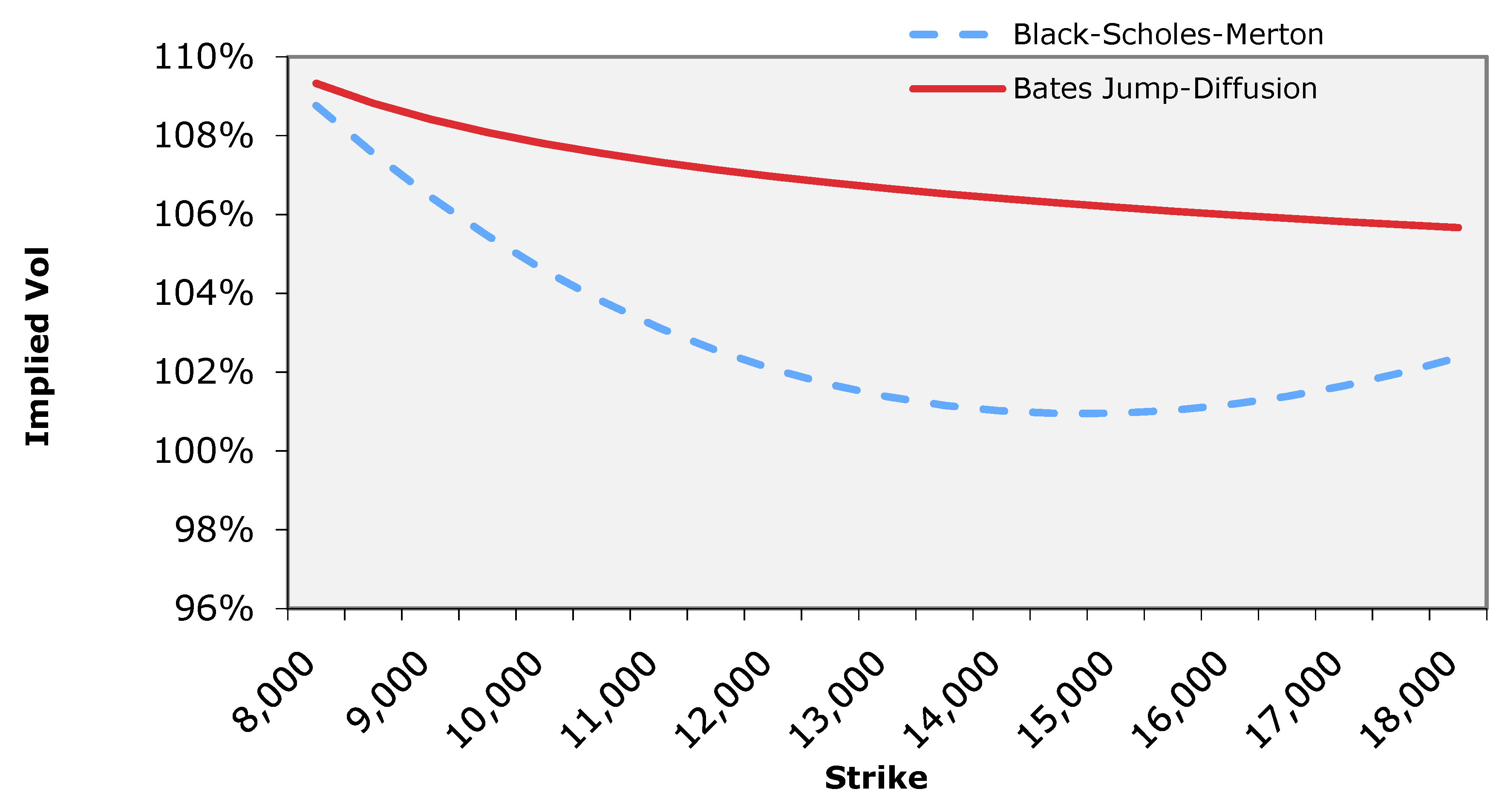
Stability across Strikes

Calibrated parameters for the Greek of above equations are set to time to maturity (τ) = 3 month(M), risk-free rate (r) = 2%, cost of carry (b) = 5%, volatility σ_B² = 0.5, jump size (kbar) = −5%, jump intensity λ = 0.124, and jump standard deviation δ = 0.02. The setting values of the asset price (S), strike price (X) for the European call option considered are 11,000 for above Figure 4A–F.

Based on the same maturities, it is clear from the graphs in Figure 5 that the parametrization of the implied volatility smile in the Bates model converges to a flat smile and is more stable across different strikes than in the Merton model. For example, in the Bates model, this convergence is possible as the smile captures the presence of jumps whereas the term structure of implied volatility is taken into account using the cost-of-carry component. Moreover, the result is in line with Mijatović and Tankov [35] regarding the function of both the jump activity index of the jump component and the diffusion process component. We should emphasize that it only serves as an illustration, to indicate that the model can yield a close fit even to a very sharp volatility phenomenon. Similar examples are discussed in Kuo [36].

5. Concluding Remarks

Overall, Bitcoin prices exhibit highly volitile behavior due to the interventions, speculative investment interest, and the numerous news-driven shocks in the market (see Scaillet et al. [17]). In this paper, we adopt the idea that Bitcoin prices are influenced by jump-diffusion and confidence about the underlying technology; as a consequence, such a jump-diffusion may spread to Bitcoin prices causing an ambiguous effect.

To describe the jump risk distribution more accurately, this paper applies the jump detection approach to identify realized jumps on the Bitcoin market and to estimate the jump parameters of intensity, mean, and variance. Crucially, similar to Tauchen et al. [37], we find that the jump intensity varies among the 2015–2018Q1 from 9.89% to 16.85%. Applying this to the Bitcoin market, this finding reports some important implications in jump frequencies and volatilities across the sample period over time.

Moreover, based on risk-neutral measures, we derive a quasi-closed formula for European-style Bitcoin derivatives under the Merton–Bates jump-diffusion risk and their Greeks, and a numerical application is provided.

To shed some light on Bitcoin hedging, this paper introduces the computation of Greeks relationships for Bitcoin options as asset replication in frictionless markets. Market makers or confidence about cryptocurrencies are not directly observed, but some major factors may be considered as target variables, such as the number and volume of Bitcoin option transactions. More unconventional problems in the current analysis are left for future research. As suggested in Figure 2A,B, we must ensure that the introduced model is capable of capturing jumps in the Bitcoin market by simply calibrating the model parameters.

As future work, we could better fit the model by incorporating the GARCH-Jump process (e.g., Chan and Maheu [38], Duan et al. [39], and Gronwald [40]) for the volatility of Bitcoin options or considering a new variable such as the stochastic volatility. Therefore, its resolution will be considerably more complex, and could be very interesting research.

References

1. Dupire, B. Pricing with a smile. Risk 1994, 7, 18–20. [Google Scholar]
2. Andersen, L.; Andreasen, J. Jump-diffusion processes: Volatility smile fitting and numerical methods for option pricing. Rev. Deriv. Res. 2000, 4, 231–262. [Google Scholar] [CrossRef]
3. Ma, Y.; Shrestha, K.; Xu, W. Pricing vulnerable options with jump clustering. J. Futur. Mark. 2017, 37, 1155–1178. [Google Scholar] [CrossRef] [Green Version]
4. He, C.; Kennedy, J.S.; Coleman, T.F.; Forsyth, P.A.; Li, Y.; Vetzal, K.R. Calibration and hedging under jump diffusion. Rev. Deriv. Res. 2006, 9, 1–35. [Google Scholar] [CrossRef] [Green Version]
5. Merton, R. Option pricing when underlying stock returns are discontinuous. J. Financ. Econ. 1976, 3, 124–144. [Google Scholar] [CrossRef] [Green Version]
6. Bates, D.S. The crash of ’87: Was it expected? The evidence from options markets. J. Financ. 1991, 46, 1009–1044. [Google Scholar] [CrossRef]
7. Cont, R.; Tankov, P. Non-Parametric calibration of jump-diffusion option pricing models. J. Comput. Financ. 2004, 7, 1–49. [Google Scholar] [CrossRef] [Green Version]
8. Gómez-Valle, L.; Martínez-Rodríguez, J. Including jumps in the stochastic valuation of freight derivatives. Mathematics 2021, 9, 154. [Google Scholar] [CrossRef]
9. Luther, W.J.; White, L.H. Can Bitcoin become a major currency? Cayman Financ. Rev. 2014, 36, 78–79. [Google Scholar] [CrossRef]
10. Yermack, M. Is Bitcoin a Real Currency? An Economic Appraisal; NBER Working Paper 19747; National Bureau of Economic Research: Cambridge, MA, USA, 2013. [Google Scholar]
11. Dowd, K.; Hutchinson, M. Bitcoin will bite the dust. Cato J. 2015, 35, 357–382. [Google Scholar]
12. Ardia, D.; Bluteau, K.; Rüede, M. Regime changes in bitcoin GARCH volatility dynamics. Financ. Res. Lett. 2019, 29, 266–271. [Google Scholar] [CrossRef]
13. Fang, L.; Bouri, E.; Gupta, R.; Roubaud, D. Does global economic uncertainty matter for the volatility and hedging effectiveness of Bitcoin? Int. Rev. Financ. Anal. 2019, 61, 29–36. [Google Scholar] [CrossRef]
14. Bouri, E.; Roubaud, D.; Shahzad, S.J.H. Do Bitcoin and other cryptocurrencies jump together? Q. Rev. Econ. Financ. 2020, 76, 396–409. [Google Scholar] [CrossRef]
15. Bouri, E.; Gkillas, K.; Gupta, R.; Pierdzioch, C. Forecasting Realized Volatility of Bitcoin: The Role of the Trade War. Comput. Econ. 2021, 57, 29–53. [Google Scholar] [CrossRef]
16. Cao, M.; Celik, B. Valuation of bitcoin options. J. Futur. Mark. 2021, 41, 1007–1026. [Google Scholar] [CrossRef]
17. Scaillet, O.; Treccani, A.; Trevisan, C. High-frequency jump analysis of the Bitcoin market. J. Financ. Econ. 2020, 18, 209–232. [Google Scholar]
18. Siu, T.K.; Elliott, R.J. Bitcoin option pricing with a SETAR-GARCH model. Eur. J. Financ. 2021, 27, 564–595. [Google Scholar] [CrossRef]
19. Jalan, A.; Matkovskyy, R.; Saqib, A. The Bitcoin options market: A first look at pricing and risk. Appl. Econ. 2021, 53, 2026–2041. [Google Scholar] [CrossRef]
20. Hilliard, J.E.; Reis, J.A. Jump processes in commodity futures prices and options pricing. Am. J. Agric. Econ. 1999, 81, 273–286. [Google Scholar] [CrossRef]
21. Kapetanios, G.; Konstantinidi, E.; Neumann, M.; Skiadopoulos, G. Jumps in option prices and their determinants: Real-time evidence from the E-mini S&P 500 option market. J. Financ. Mark. 2019, 46, 100506. [Google Scholar]
22. Qiao, G.; Yang, J.; Li, W. VIX forecasting based on GARCH-type model with observable dynamic jumps: A new perspective. N. Am. J. Econ. Financ. 2020, 53, 101186. [Google Scholar] [CrossRef]
23. Lee, S.S.; Mykland, P.A. Jumps in financial markets: A new nonparametric test and jump dynamics. Rev. Financ. Stud. 2008, 21, 2535–2563. [Google Scholar] [CrossRef]
24. Dumitru, A.-M.; Urga, G. Identifying Jumps in Financial Assets: A Comparison Between Nonparametric Jump Tests. J. Bus. Econ. Stat. 2012, 30, 242–255. [Google Scholar] [CrossRef] [Green Version]
25. Huang, X.; Tauchen, G. The relative contribution of jumps to total price variance. J. Financ. Econ. 2005, 3, 456–499. [Google Scholar] [CrossRef]
26. Cheang, G.H.L.; Chiarella, C. A Modern View on Mertons Jump-Diffusion Model; Research paper No. 287; University of Technology Sydney, Quantitative Finance Research Centre: Sidney, Australia, 2011. [Google Scholar]
27. Geman, H.; EI Karoui, N.; Rochet, J.C. Changes of numeraire, changes of probability measure and option pricing. J. Appl. Probab. 1995, 32, 443–458. [Google Scholar] [CrossRef]
28. Bannör, F.K.; Scherer, M. Capturing parameter uncertainty with convex risk measures. Eur. Actuar. J. 2013, 3, 97–132. [Google Scholar] [CrossRef]
29. Haug, E.G. The Complete Guide to Option Pricing Formulas, 2nd ed.; McGraw–Hill: New York, NY, USA, 2007. [Google Scholar]
30. Beckers, S. A note on estimating the parameters of the diffusion–jump model of stock returns. J. Financ. Quant. Anal. 1981, 16, 127–140. [Google Scholar] [CrossRef]
31. Ball, C.A.; Torous, W.N. A simplified jump process for common stock returns. J. Financ. Quant. Anal. 1983, 18, 53–65. [Google Scholar] [CrossRef]
32. Duan, J.C.; Ritchken, P.H.; Sun, Z. Jump Starting GARCH Pricing and Hedging Option with Jumps in Returns and Volatilities; Working Paper; National University of Singapore: Singapore, 2007. [Google Scholar]
33. Cretarola, A.; Figà-Talamanca, G.; Patacca, M. Market attention and Bitcoin price modeling: Theory, estimation and option pricing. Decis. Econ. Financ. 2020, 43, 187–228. [Google Scholar] [CrossRef] [Green Version]
34. Tankov, P.; Voltchkova, E. Pricing, Hedging, and Calibration in Jump-Diffusion Models. In Frontiers in Quantitative Finance; Cont, R., Ed.; Wiley: Hoboken, NJ, USA, 2008. [Google Scholar] [CrossRef]
35. Mijatović, A.; Tankov, P. A new look at short-term implied volatility in asset price models with jumps. Math. Financ. 2016, 26, 149–183. [Google Scholar] [CrossRef] [Green Version]
36. Kou, S.G. A jump-diffusion model for option pricing. Manag. Sci. 2002, 48, 1086–1101. [Google Scholar] [CrossRef] [Green Version]
37. Tauchen, G.; Zhou, H. Realized jumps on financial markets and predicting credit spreads. J. Econ. 2011, 160, 102–118. [Google Scholar] [CrossRef] [Green Version]
38. Chan, W.H.; Maheu, J.M. Conditional Jump Dynamics in Stock Market Returns. J. Bus. Econ. Stat. 2002, 20, 377–389. [Google Scholar] [CrossRef]
39. Duan, J.-C.; Ritchken, P.; Sun, Z. Approximating GARCH-jump models, jump-diffusion processes, and option pricing. Math. Financ. 2006, 16, 21–52. [Google Scholar] [CrossRef]
40. Gronwald, M. Is Bitcoin a Commodity? On price jumps, demand shocks, and certainty of supply. J. Int. Money Financ. 2019, 97, 86–92. [Google Scholar] [CrossRef]
41. Chen, K.-S. Research on Equity Release Mortgage Risk Diversification with financial innovation: Reinsurance Usage. J. Risk Model Valid. 2016, 10, 35–55. [Google Scholar] [CrossRef]
42. Chen, H.Y.; Lee, C.F.; Shih, W.K. Derivation and application of Greek letters: Review and integration. In Handbook of Quantitative Finance and Risk Management, Part III; Springer: Berlin/Heidelberg, Germany, 2010; pp. 491–503. [Google Scholar]
Figure 1. Market Price of Bitcoin in the Bitcoin/USD exchange rate from 1 January 2015 to 28 February 2018. Notes. Jump effect of Bitcoin price revaluation on Bitcoin/USD exchange rate, huge jump starting from Q3/2017.
Mathematics 09 02567 g001
Figure 2. Return, Logarithmic Returns of Bitcoin. The top panel of the graph illustrates the daily returns of Bitcoin over the period time and the bottom panel of the graph illustrates the daily logarithmic returns of Bitcoin.
Mathematics 09 02567 g002
Figure 3. Time series of the Bipower variation, realized volatility, and the relative jump and jump statistic component for Bitcoin prices. The top panel of the figure depicts the BVt (Equation (4)), the second panel plots for respective graphs the daily realized volatility RVt (Equation (3)); the third panel plots the relative jump component RTt (Equation (6)); and the bottom panel depicts the jump statistic (i) (Equation (7)) at significance α = 0.05.
Mathematics 09 02567 g003aMathematics 09 02567 g003b
Figure 4. (A) The surface of Call options’ Delta; (B) The surface of put options’ Delta; (C) The surface of call and put options’ Gamma; (D) Implied volatilities for call and put options’ Vega; (E) Volatility surface of call options’ Rho on Bitcoin price; (F) Theta of European call options.
Mathematics 09 02567 g004
Figure 5. Volatility Smile Fitting. Figure depicts the volatility smile that the parametrization of the implied volatility smile in terms of the strike. This figure plots implied volatilities of call options on the Bitcoin price index as a function of their strikes and maturities for the Bates’ model (red solid line) and the BSM model (blue dotted line). More importantly, the Bates’ volatility jump-diffusion model is consistent with an asymmetric volatility smile. This model assumes jump risk is systematic and appears to be a much closer match to reality than Merton due to the simultaneous asset price jumps and amplitudes, possibly by varying amounts.
Mathematics 09 02567 g005