Abstract
The normal distribution and its perturbation have left an immense mark on the statistical literature. Several generalized forms exist to model different skewness, kurtosis, and body shapes. Although they provide better fitting capabilities, these generalizations do not have parameters and formulae with a clear meaning to the practitioner on how the distribution is being modeled. We propose a neat integration approach generalization which intuitively gives direct control of the body and tail shape, the body-tail generalized normal (BTGN). The BTGN provides the basis for a flexible distribution, emphasizing parameter interpretation, estimation properties, and tractability. Basic statistical measures are derived, such as the density function, cumulative density function, moments, moment generating function. Regarding estimation, the equations for maximum likelihood estimation and maximum product spacing estimation are provided. Finally, real-life situations data, such as log-returns, time series, and finite mixture modeling, are modeled using the BTGN. Our results show that it is possible to have more desirable traits in a flexible distribution while still providing a superior fit to industry-standard distributions, such as the generalized hyperbolic, generalized normal, tail-inflated normal, and t distributions.
1. Introduction
Flexible modeling is an ongoing study in distribution theory that dates back as long ago as 1879, when Galton pioneered the log-normal distribution [1]. Since then, the field has exploded with new distributions and ways of generating them. These models include finite mixture models [2], variance-mean mixtures [3], copulas [4], the Box–Cox transformation [5], order-statistics-based distributions [6], probability integral transformations of [7], and the Pearson system of distributions [8], to name but a few. The impact of flexible modeling is further underscored by their successful integration into classical statistical approaches, such as time series analysis [9], space-state models [10], random fields [11], regression models [12], linear mixed-effects models [13], non-linear mixed-effects models [14], Bayesian statistics [15], and Bayesian linear mixed models [16]. In [17,18,19], some of the desirable traits of a univariate flexible model are formulated. We focus on three highlights that the authors have in common:
- A finite number of well interpretable parameters: These include parameters that specifically control location, scale, skewness and kurtosis.
- Favorable estimation properties: It is important that the parameters can be estimated correctly to ensure correct predictions and inferences from the model. Inferentially speaking, the ideal would be to have a model to use in tests of normality.
- Simple tractability: Closed-form expressions are still desirable, despite modern computational power. Simple formulae describing characteristics of distributions aid in exposition and additionally improve computational implementation and speed.
- Finite moments: Most real-world measurements require this property.
To this end, a systematic bottom-up approach is to be taken to specify a new flexible model. A flexible model is commonly made up of a symmetric base model to which a skewing parameter is added, as is the case with Azzalini skewed distributions [20], order-statistics-based distributions [6], and transformation approaches, see [21,22,23,24]. The body and tail properties of a skewed model are heavily dependent on the chosen base model, since the skewing mechanism is intended to accommodate the skewness, and not necessarily the heavy tails in the data. The motivation for the body-tail generalization of the normal distribution would be to provide a new symmetric model with the aforementioned desirable traits for symmetric data, and serve as a new base model for further generalizations to accommodate skew data in the future.
The paper is structured as follows. Section 2 gives a short overview of the generalized normal distribution (GN), which will be generalized. Section 3 introduces a derivative kernel method of generalizing known distributions. Section 4 consists of the derivations for the body-tail generalized normal (BTGN), density function, cumulative probability function (CDF), moments, moment generating function (MGF). Section 5 gives background on maximum likelihood (ML), maximum product spacing (MPS), seasonally adjusted autoregressive (SAR) models, and finite mixtures models of BTGN. Section 6 applies the BTGN to log-returns data, a SAR model to minute average wind speeds, and a two-component finite mixture model to annual wind speed data. Finally, Section 8 concludes with final remarks and observations.
2. The Generalized Normal Distribution
This contribution generalizes the known GN distribution further. The latter has been referred to by many names, such as exponential power, generalized power, generalized error, and generalized Gaussian. This family is originally proposed by [25], and later on again by [26,27,28]. A complete review of the GN is given by [29]. The GN density function is given below:
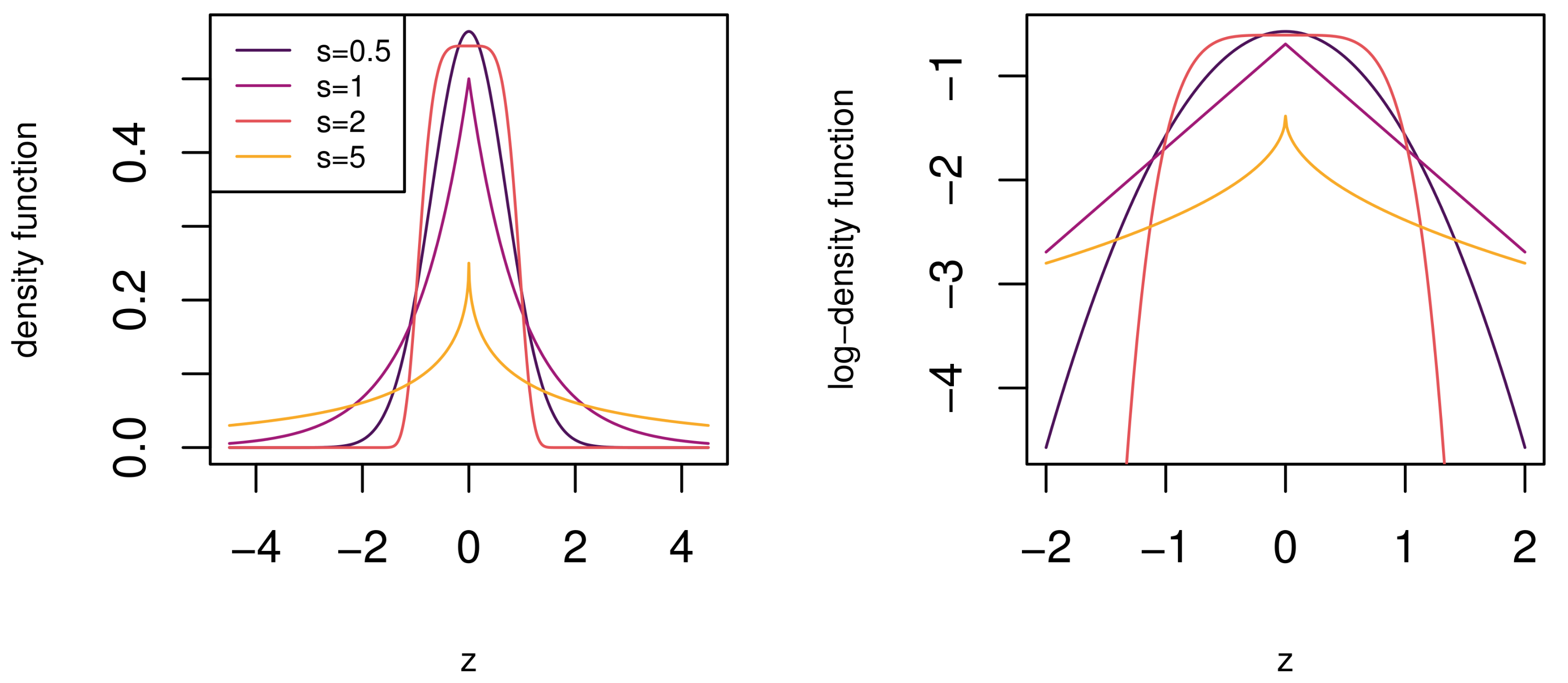
and . From (1), it is clear that it contains the normal, Laplace, and uniform distributions are sub-models of the GN for shape parameter values of , , and , respectively. From Figure 1, it can be seen that for smaller values of s, the GN is more heavy-tailed and more light-tailed for larger values of s.
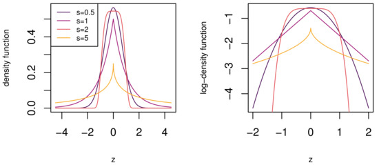
Figure 1.
The generalized normal (GN) density function for different values of s. The GN density function is relatively heavy-tailed for values of and light-tailed for values .
A significant limitation of the GN must be noticed here. The body shape cannot be adjusted separately from the tail shape. Fixed body and tail shapes are common among distribution generalizations. For instance, the normal, Laplace, logistic, t, [30], and hyperbolic (HYP) [31] distributions have either fixed body or tail shapes, respectively. Subsequently, in the next section, we provide a new body-tail generalization of the normal distribution that provides different body and tail shape combinations. The intent of this generalization is to provide a new base model for skew generalizations, as discussed in Section 1, and for fitting a more comprehensive range of data types, as will be shown in Section 6.
3. Modifying Distributions through Their Derivative Kernel Functions
The construction is based on the relationship between the derivative kernel function and the density function. Given some “appropriate” derivative kernel function, , a new distribution can be generated by simply integrating and normalizing the resulting function to give a new density function . To the best of our knowledge, this particular type of deliberate integration of a derivative kernel function has not been done before. The procedure followed for the generalization of the GN kernel is as follows:
- Calculate the derivative kernel function for the GN.
- Inspect the functional components of the kernel function to understand which properties can be changed or generalized.
- Take the indefinite integral of the derivative kernel function.
Note that simple derivative kernels simplify subsequent mathematical operations, as is the case for the BTGN. Since the t-distribution generalizes the normal distribution with heavier tails, we use it as an introduction to tail behaviour from a derivative kernel perspective.
According to Figure 2, for heavier tails and lower degrees of freedom , the derivative kernel function has higher magnitudes in the tail and lower magnitudes at the body of the function. Next, we study the derivative of the GN distribution kernel from (1)
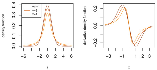
Figure 2.
The density and derivative density functions of the t-distribution. Note the different density derivative function magnitudes at the body and tail for lighter and heavier tails.
The kernel is proportional to two main factors— and . Since these factors have a fixed relationship with , we can generalize the kernel by breaking the relationship. Replacing with in (2), we have a new more general derivative kernel
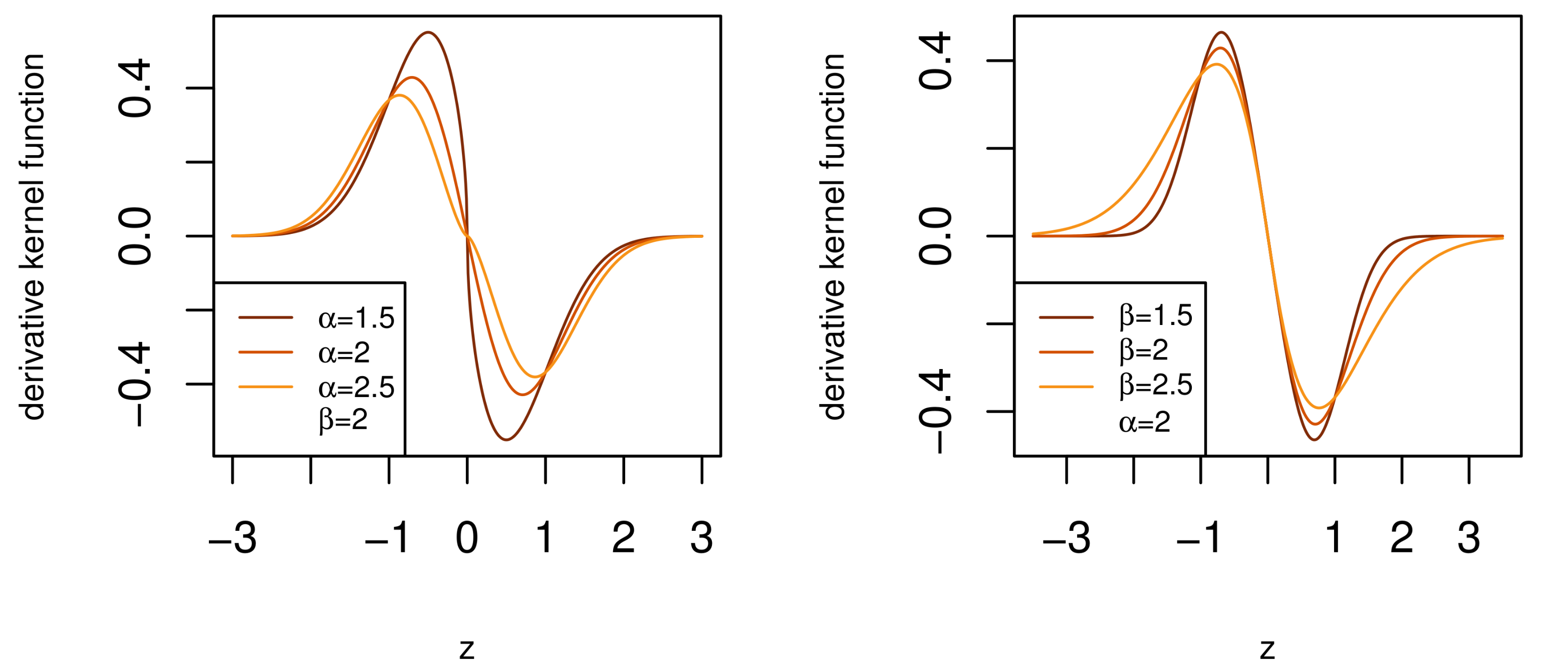
where with . In Figure 3 the effect of the additional parameter of (3) is shown. For a fixed value of , the parameter controls the shape of the body, making it “sharper” or “flatter” in a similar fashion to the parameter s of the GN distribution, see Section 1. Likewise, for a fixed value , , the parameter controls the shape of the tails, making them lighter or heavier. The derivative kernel in (3) has therefore achieved separate control of the body and tail shape of the distribution.
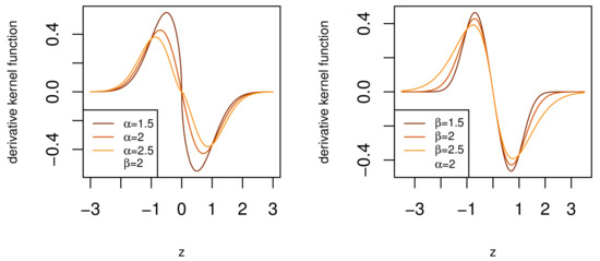
Figure 3.
The derivative kernel function of body-tail generalized normal (BTGN) distribution.
Importantly, the role of is very similar to in the t-distribution, but with a wider range, which includes lighter than normal tails for , which is advantageous in flexible modeling. This is clear from the higher and lower magnitudes of the derivative kernel function in the tails for different values of , see Figure 3. This derivative kernel (3) lays the foundation for the BTGN distribution that will, by definition, contain the GN distribution, for , and has separate control of the body and tail shape. The latter makes the BTGN an ideal candidate for body and tail shape tests for normality in future research. In Section 4, the density function will be derived from (3), as well as various other statistical properties.
4. The Body-Tail Generalized Normal Distribution
In this section, the BTGN is defined, and various properties are derived, such as the density function, CDF, moments, MGF, and ML equations.
4.1. Density Function
Let the standard BTGN derivative kernel function be defined by (3) for . The indefinite integral of (3) is evaluated by making the transformation and the definition of the upper incomplete gamma function to get
where is the upper incomplete gamma function, see ([32], p. 899). The indefinite integral of given by (4) yields a new symmetric kernel function
The normalizing constant for in (5) is given by direct substitution of Lemmas A1 and A2 in Appendix A
normalizing the kernel function with (6) gives the standard BTGN density function below
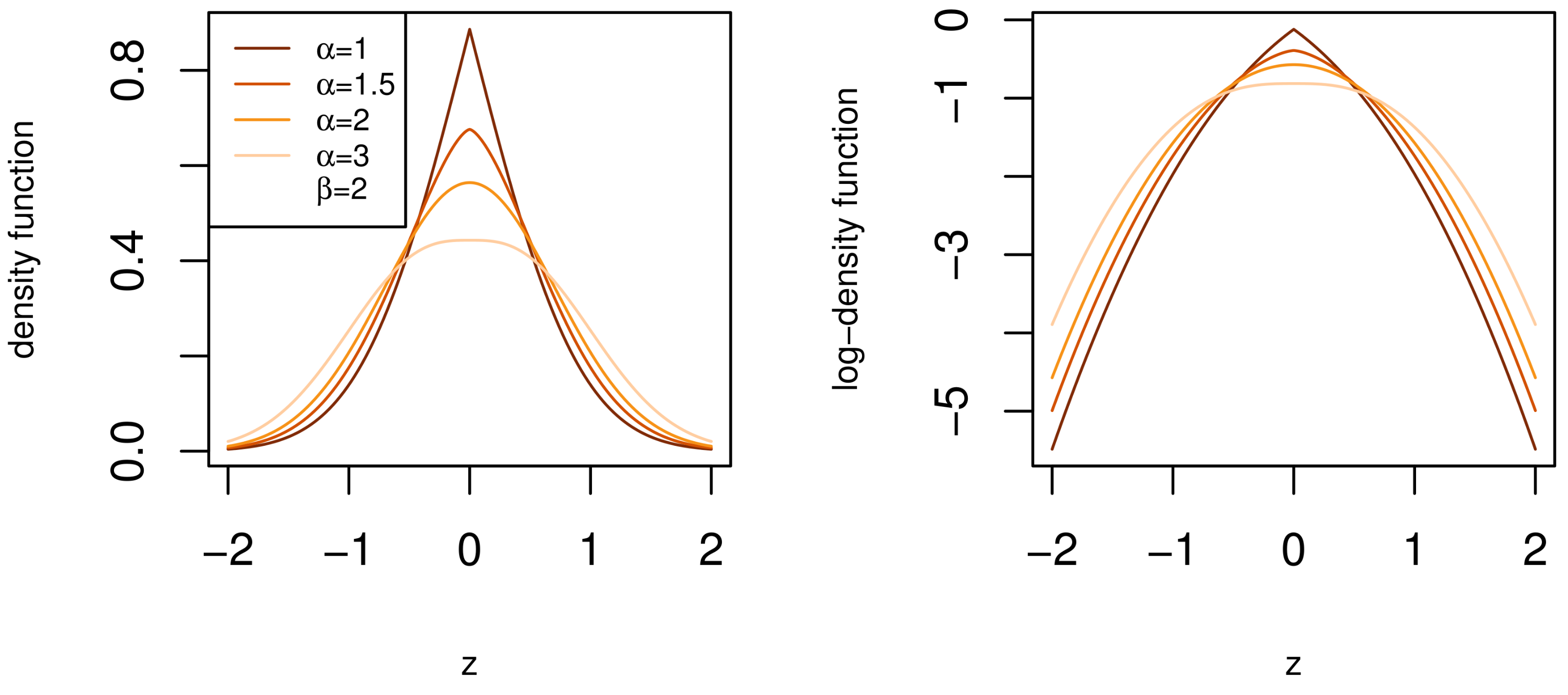
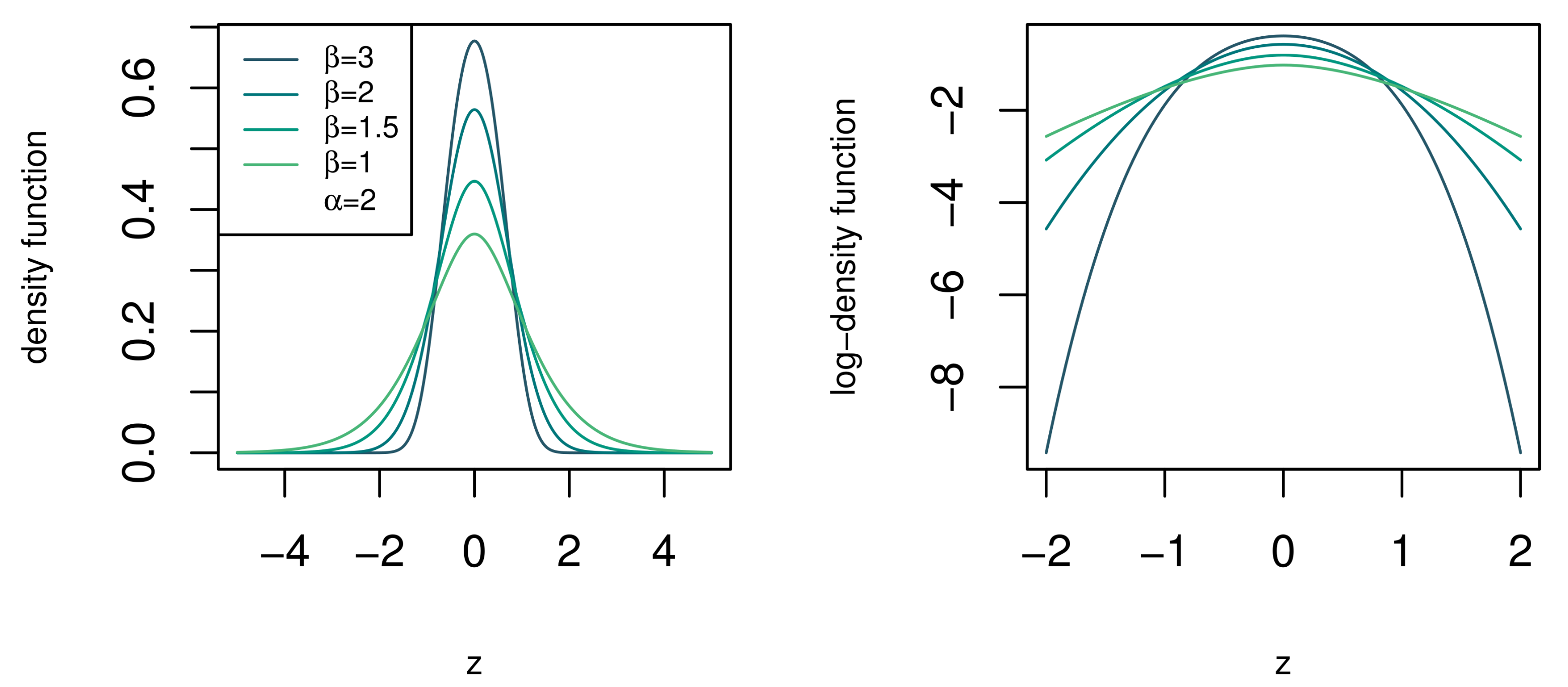
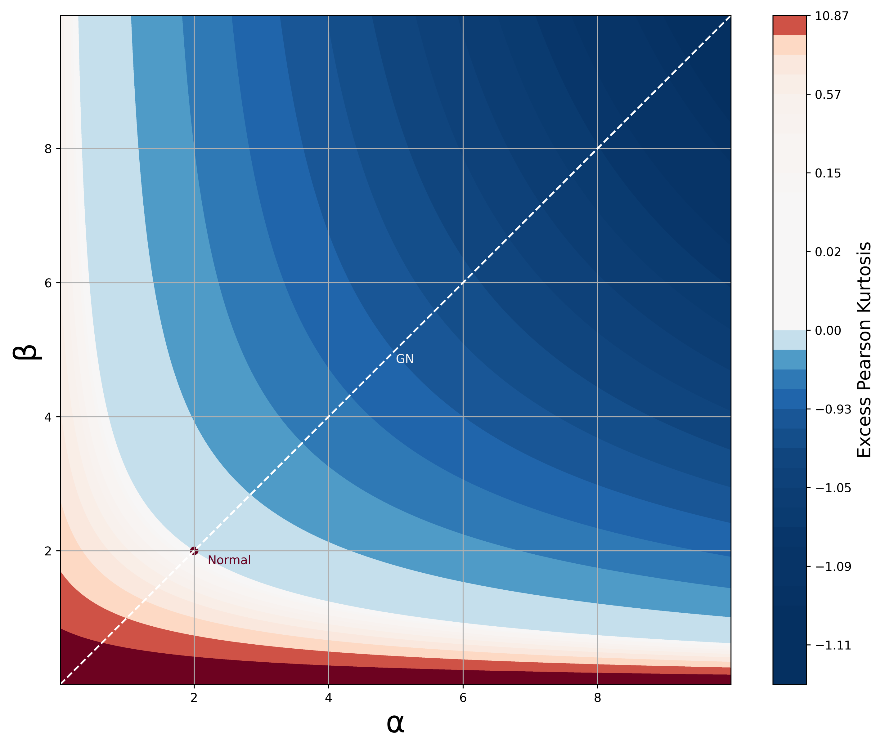
where and . Referring back to the desirable traits in Section 1, the density function, CDF, and moments of the BTGN consist of very well known special functions and satisfy the desirable trait of simple and closed-form expressions. The BTGN density function is depicted for different combinations of its parameters in Figure 4 and Figure 5. For a fixed body shape of , values of are more heavy-tailed than the GN distribution with , and more light-tailed for values of . The excess Pearson kurtosis for the BTGN, GN, and normal distribution is depicted in Figure 6, confirming the latter properties. The range of different body or tail shapes for a given level of kurtosis has been generalized to contours on the plane for the BTGN. Although different levels of kurtosis can be achieved on straight line combinations of , the body and tail shapes cannot vary.
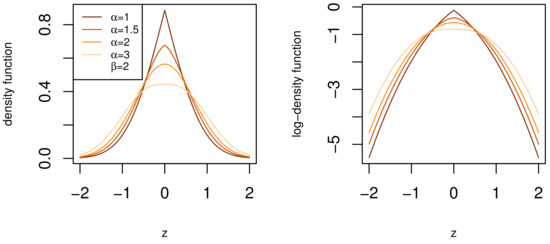
Figure 4.
The density function of the BTGN distribution for different body shapes for a fixed tail shape of .
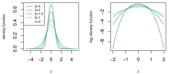
Figure 5.
The density function of the standard BTGN for different tail shapes of for a fixed body shape of .

Figure 6.
Excess Pearson Kurtosis for the BTGN distribution for different values of and . Excess kurtosis of zero is equal to the normal distribution kurtosis.
Again, it can be verified that if , we have the regular GN distribution, as discussed in Section 2:
This fact implies that for , we have a normal distribution with scale, , and the Laplace distribution for respectively. This implies that the BTGN can be used for tests of normality of distributions with different body and tail shapes, giving it another desirable trait. For comparison, two other candidate distributions that include the normal distribution come to mind; the t and generalized hyperbolic (GYHP) distributions [31]. These are well-documented distributions that both lack separate control of the body and tail shape. The former can not model lighter than normal tails and has a fixed normal-like body shape. The latter has shape parameters that interact to give different body and tail shape combinations [33]. The BTGN, therefore, excels at the desirable trait of a finite number of well interpretative parameters. Finally, the location-scale BTGN density function is derived using the transformation
and is denoted as from here on forward.
4.2. Characteristics
The CDF of the standard BTGN, , is easily calculated from (7) using Lemma A2 in Appendix A for
and for
Next, the moments are derived using the moments of the standard BTGN. Noting that any odd moment of the standard BTGN is zero. The absolute rth moment of the standard BTGN is derived from (7) by direct substitution of Lemma A2 in Appendix A
Then, the rth moment is a function of (11) and the binomial expansion of a polynomial ([32], p. 25)
where if r is odd and if r is even. The mean, variance, and Pearson kurtosis for the BTGN are then given as
A numerical expansion of the MGF is derived for completeness and the for calculating moments of log-transformed BTGN data. That is, for a distribution . The rth moment of Y is given by , the MGF of X evaluated at r. Starting with the MGF of the standard BTGN, from (7) and the series expansion of the hyperbolic cosine function ([32], p. 28)
Finally, from (11)
Therefore, MGF for
5. BTGN Estimation Procedures
This section proposes estimation procedures for fitting finite mixtures and SAR times series models based on the BTGN using ML and MPS estimation. The updated ML estimation is well known, and we elaborate more on MPS estimators. MPS estimators are similar to ML estimators, in that they are estimators of Kullback–Leibler divergence, consistent estimators, and are at least as asymptotically efficient as ML estimators, where the latter exist [34]. The MPS method of parameter estimation was developed independently by [35,36]. The motivation for MPS estimation is based on the probability integral transform: that any sample of independent and identically distributed observations should be uniformly distributed and therefore uniformly “spaced” with respect to the distribution CDF from which they were sampled. By maximizing the geometric mean of these spacings with respect to the distribution parameters, MPS estimates are obtained.
5.1. ML Estimation
The log-likelihood (LL) for a random sample from observations is
using (8). The ML estimates are given as the solution of the parameters for the partial derivatives of (17) set to zero. The derivatives with respect to individual terms inside the sum of (17) are given in Appendix B.
5.2. MPS Estimation
For an ordered random sample of size n from a distribution with unknown parameters and CDF . The sample spacings are given by:
where , for . The MPS estimates of is defined as a value that maximizes the logarithm of the geometric mean of sample spacings:
In situations where repeat observations are present, Equation (18) will lead to infinite values in the logarithm of Equation (19). To counter this problem, [35] suggests using density function of the distribution, for values of i that are repeated. Next, maximizing Equation (19) requires partial derivatives of the form
for each . The partial derivatives in (20) are set to zero and solved analytically or numerically to yield MPS estimates. In cases where repeat values are encountered, the partial derivatives of the individual terms are equal to the LL derivatives. The partial derivatives within the individual terms of (20) for the BTGN are given in Appendix B.
5.3. Fitting Mixtures of BTGN
Finite mixture models are helpful in situations where the data have more than one sub-group, for which the sub-groups cannot be individually identified and separately analyzed. Here, we outline the use of the BTGN in this context. The density function of a k component finite mixture of body-tail generalized normal (FMBTGN) distributions is a function of (8), as given below
where, , , and . The LL for a random sample from a k component FMBTGN observations is
where is given in (8). Due to the summation within the logarithm of (22), direct optimization may be cumbersome. Therefore we follow a modified expectation maximization (EM) algorithm based on [37]. In order to use the EM algorithm, an unobserved indicator variable
is introduced into (22) to replace the mixing proportion. Then the conditional expectation to be maximized is
The expectation step equation is
and the maximization step equations are:
It is clear that (24)–(28) are weighted functions of (A5)–(A8) in Appendix B. For a detailed guide to implementing the EM algorithm, see [38,39]. The normal approach to implementing the EM for optimization would consist of an estimation step and a maximization step, which is iteratively used to update the parameters until convergence. The modified EM used for fitting k component FMBTGN works by updating the location and scale parameters separately from the shape parameters, as described in the Algorithm A1 in Appendix C. Similar to most EM-based algorithms, the final estimates are sensitive to initial starting values and provide a local optimum [40]. Since the normal distribution is a special case of the BTGN, a fitted finite k component mixture of normal can serve as initial values of with .
5.4. Fitting SAR Models
Seasonality and autoregressive innovations are commonly observed in many time series data. Here, we outline a simple model using the BTGN in this context. A basic autoregressive model of order p defines the process with a linear combination of p lagged terms as
for time intervals of where are AR parameters, and is white noise with scale and shape parameters, , respectively. Additionally, the process mean is given by and for stationary AR processes, the roots of the characteristic equation
are all greater than one [41]. The adjustment for seasonality is done by the addition of sine-cosine pairs for a cyclical adjustment of the process mean for seasonal cycles of frequencies for as
This process is denoted as from here on. The joint density function of is intractable since these random variables are linear combinations of each other. However, the joint density function can be approximated by the conditional joint density function of
where is the scale and shape parameters of the white nose. The conditional ML estimates are given by maximizing the log of (35). Similarly, the conditional MPS estimates are given by
where , , is defined by (18), and the ordered values of (36). The model estimates are then found as explained in Section 5.2.
6. Application
In this section, the BTGN is used in a real-world application, showing the need for flexible distributions and the benefits they have to existing fields of study. The evaluation of fit is done by computing both in-sample and out-of-sample validation metrics. The in-sample statistics are Akaike information criterion () and Bayesian information criterion (), and it is computed on the subset of data used for estimation. The out-of-sample validation is the computed a subset of data excluded from estimation. This ensures robust goodness of fit analysis and prevents the overfitting of the final models. Overall, we illustrate the wide applicability of the BTGN in a variety of applications by the use of different competitor distributions and estimation techniques in each data modeling situation. All applications are implemented using packages NumPy [42], Scipy [43], and mpmath [44] in Python. All the above is applicable unless stated otherwise.
6.1. Financial Risk Management and Portfolio Selection
Flexible modeling is particularly relevant to risk management and portfolio selection when modeling stock prices and asset returns. Many empirical studies have shown and cautioned using the normal distribution to determine risk factors in these areas, see [45,46]. The main criticisms are symmetry and thin tails [47]. The former is not necessarily a limitation [48], and the latter is considered more harmful. Therefore, numerous alternative distributions have been suggested, such as the -stable sub-Gaussian (ASSG) distributions [49], GHYP, and sub-models of the latter such as the HYP, normal inverse Gaussian (NIG), variance Gamma (VG), and t distribution [50]. The ASSG is so heavy-tailed that the second moment is infinite, inconsistent with empirical findings [47]. Many theoretical models in finance require the existence of this moment [51]. When using the t distribution, the estimated degrees of freedom may be so low that either the second or fourth moment may not exist. The GHYP is a very impressive distribution with high flexibility and various sub-models. However, the density function of the GHYP is very complicated, with many different parametrizations, see (38). Up to four parametrizations with limited interpretations are discussed by [52] alone. The BTGN can be considered an improvement by having finite moments (11), a simple density function, and interpretable parameters. Validating the empirical usefulness of the BTGN, we compare the performance of BTGN with the symmetric versions of the GHYP, NIG, VG, t, and GN distributions on real financial data.
Stock Returns Data
The data consist of daily log-returns for the shares of three companies listed on the NASDAQ, each in different market sectors. The companies are CASI Pharmaceuticals, Inc. (CASI), iShares S&P (ISHG), and Partner Communications Company Ltd. (PTNR). The period for the data is 4 January 2016 to 31 December 2020, available online http://finance.yahoo.com, accessed 20 September 2021. In Table 1, the summary statistics and the Jarque–Bera test statistics for normality are given for each stock. It is observed that all the series are leptokurtic, and the Jarque–Bera statistic confirms the departure from normality at a 1% significance level. The returns distributions are fitted using ML estimation, and the ghyp package in R [53] with the simplifying assumption of independence of observations. For the validation of results, we use the in-sample criterion computed on the entire sample and an extra verification with out-of-sample LL calculated on the last 20% of the data time range, which was excluded during estimation.

Table 1.
Summary statistics for log-returns data.
6.2. Returns Distributions
The competing models against the BTGN are the GHYP and nested models. The density function of the GHYP is given as
where is the modified Bessel function of the third kind and . The domains of variation of the parameters are , and
The fourth, , parametrization from [52] is used, where and . Note, that we fix for symmetric distributions. If X follows a distribution such as (38), we write . Then, the nested models are given by as the HYP distribution, as the NIG distribution, as the VG distribution, and as the t distribution.
6.3. Results
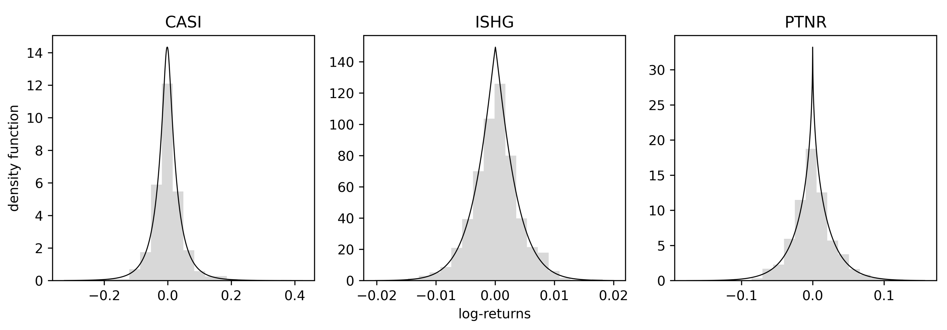
In Table 2, the in-sample criterion, out-of-sample LL, and fitted ML estimates are given. The and are the lowest for the BTGN, and the is the highest for the BTGN distribution. It can therefore be concluded that the BTGN distribution fits best. Interpreting the BTGN body parameters, the values of show that all the body shapes are “sharper” than normal. Interpreting the BTGN tail parameters, the values of show that all the tail shapes are thinner than a fixed GN body shape would accommodate. The departure from the normal distributional shape is also evident in Figure 7, where the fitted BTGN density functions are shown. Finally, comparing the BTGN to the fitted t distributions, for the ISHG stock, the second and higher moments are infinite, and for the CASI stock, the fourth moment is infinite, which will not be the case for the BTGN.
Table 2.
Table of distributions fitted to log-returns data with in-sample criterion and out-of-sample log-likelihood (LL).

Figure 7.
Fitted BTGN density functions to log-returns data.
7. Wind Energy
In the sector of renewable energy generation, wind energy has seen remarkable growth. Annual wind energy generation grew by 2,477,646% from 1985 to 2020, with a current all-time high of 1591.2 Terra-watt hours in 2020 [54]. The cost of wind energy has also decreased dramatically, with some estimates of global weighted average levelized cost of electricity reducing by 88% from $0.40 to $0.05 in 2016 $/kilowatt-hour [54]. Keeping in mind the pressure mounting from the Intergovernmental Panel on Climate Change on governments to take immediate steps to blunt the catastrophic impacts of global warming, we expect this field of study to be relevant in the foreseeable future. The wind energy application consists of basic short and long-run model analyzes for the initial investigation into the wind distribution at a particular site. This is for the daily operations of a wind farm, as well as the suitability of a site for a wind farm. We fit a SAR time series model for hourly wind speed data readings and a two-component finite mixture to make inferences of the annual available wind energy.
7.1. Wind Speed and Power Distributions
The distribution of wind speed W determines the amount of energy available at a particular site. The power distribution E is a cubic function of the wind speed
where is the density of air and A is the sweep area of the wind turbine ([55], p. 6). The expected wind energy is thus dependent on the third moment of the wind speed distribution. The estimated (expected) power of a site is thus very sensitive to the fitted distribution because of this cubic relationship, making it an ideal application of a more flexible model. The most common and comparable industry models are the normal and log-normal distributions [56], since they are both based on symmetric uni-modal distributions. The short-run wind speed distribution will be modeled by a SAR model using different comparable white noise distributions. For the long-run (annual) wind speed distribution, we use two-component mixtures on the log of the wind speed data. This is done because it is common for a particular wind site to have two different wind climates for summer and winter ([55], p. 16), [56].
7.2. Wind Speed Data
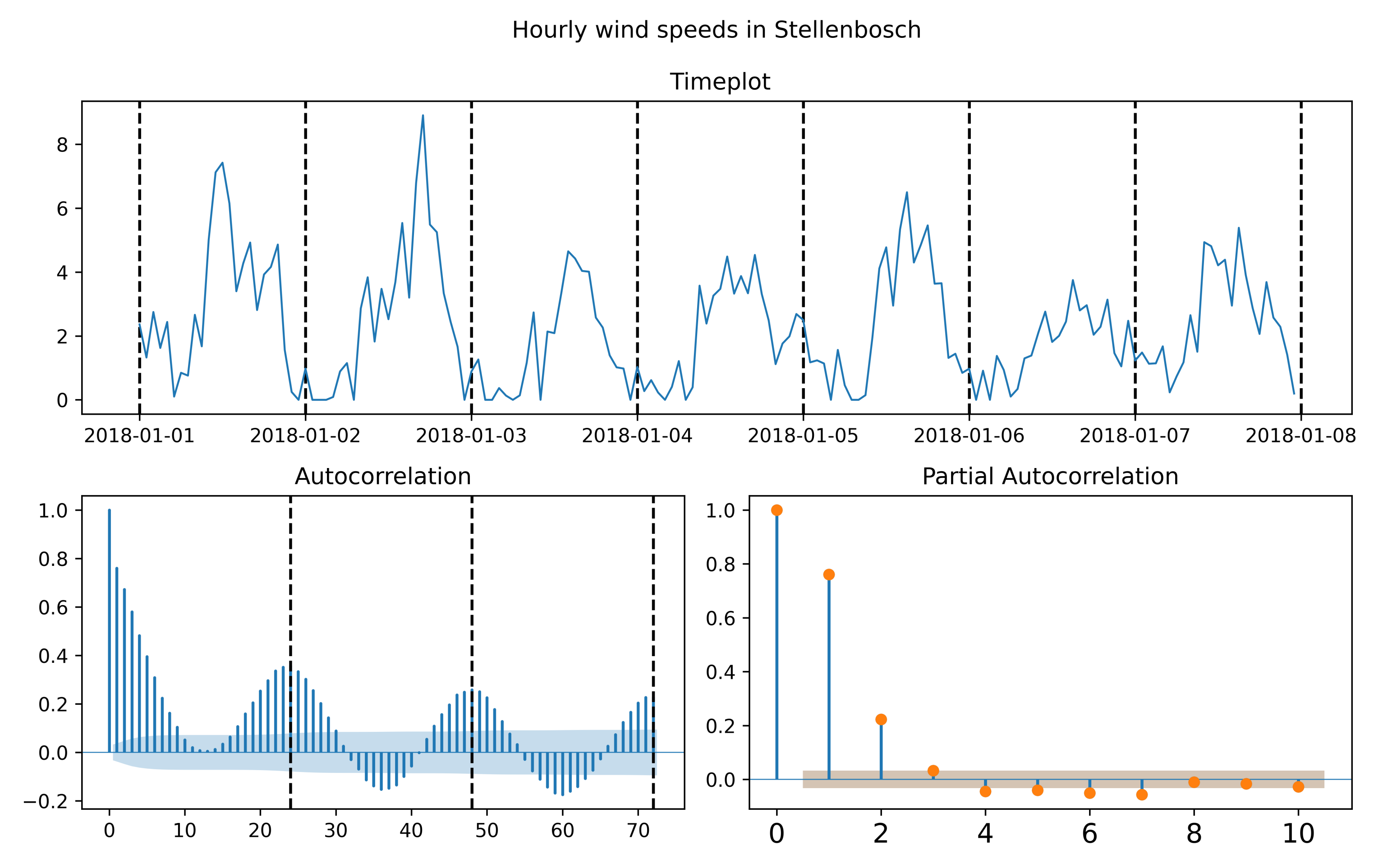
The data consist of hourly one minute average wind speed measurements in from the University of Stellenbosch located at latitude: −33.92810059, longitude: 18.86540031 in South Africa available online https://sauran.ac.za, accessed 1 August 2021. The Cape province has four wind farms in the area around Cape Town and Stellenbosch, see https://sawea.org.za/wind-map, accessed 1 August 2021. The data date ranges for two years, from 1 January 2017 to 1 January 2021. In Table 3, the summary statistics of the annual wind data are given, which is relevant to the long-run application. In Figure 8, a depiction of the hourly minute average readings is given in a time plot, and the correlation structure is depicted by the autocorrelation function (ACF) and partial autocorrelation function (PACF) for the short-run application.
Table 3.
Summary statistics for annual wind data.
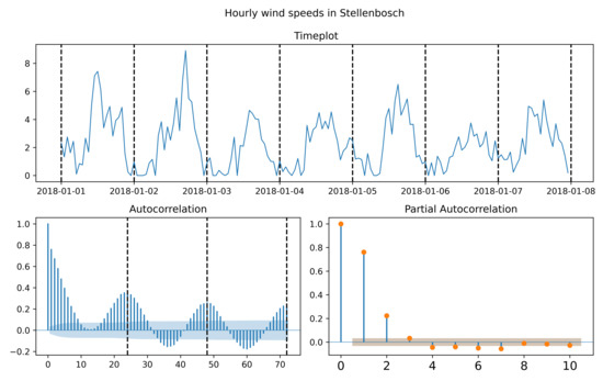
Figure 8.
Timeplot, autocorrelation function (ACF), partial autocorrelation function (PACF) of hourly wind speed measurements in Stellenbosch.
7.3. Short-Run Wind Speed Model
The process in question is hourly wind speed measurements in m/s for the time period 1 January 2018 to 1 June 2018. In Figure 8, two important phenomena are observed. In the autocorrelation function (ACF), a strong 24-h seasonality is shown, and in the PACF, the first two lags are most significant. Therefore, we proceed in fitting an model using different white noise and MPS estimation, with repeat measurements described in Section 5.4. The out-of-sample subset is taken as the last 25% of data time range excluded during estimation.
7.3.1. White Noise Distributions
The comparative white noise for the model is chosen as the normal and GN distribution, since it is a nested model of the BTGN. Since these comparative models do not have separate control of their body and tail shape, it can be shown that this additional control is useful for the application.
7.3.2. Results
The in-sample criterion, out-of-sample LL, and fitted MPS estimates are tabulated in Table 4. The and are the lowest for the BTGN, and the is the highest for the model using BTGN white noise. It can therefore be concluded that the BTGN model fits best. In general, the data are more heavy-tailed than what the normal distribution can accommodate, as can be seen from both the GN and BTGN tail shape . However, a “flatter” than normal body shape has been fitted using the BTGN since , which the GN can not achieve with a fixed body shape. In Figure 9, the residuals for the fitted model are shown. In the histogram, the “flatter” than normal body is evident, as well as some possible skewness for which a symmetric BTGN can not account. From the ACF and PACF, there are very slight auto and partial autocorrelations remaining. For parsimony and practical purposes, additional parameters are not considered.
Table 4.
Fitted models with in-sample criterion and out-of-sample LL.
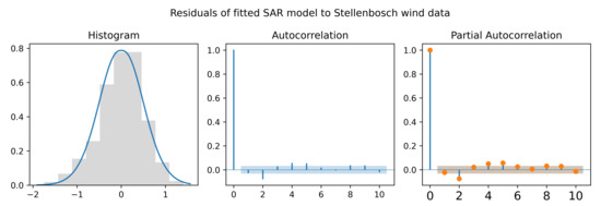
Figure 9.
Timeplot, ACF, and PACF of residuals for fitted seasonally adjusted autoregressive model.
7.4. Long-Run Wind Speed Model
The data in question are the full data set of hourly wind speed measurements. Two-component finite mixtures are fitted to the log of the data using the EM and modified EM Algorithm A1 in a two-step process. The initial estimation is done on the full data with the computation of the in-sample criteria. Thereafter, a ten-fold cross-validation approach is used on the full set of data. That is, for each randomly selected fold, a two-component mixture is fitted, and the LL is calculated on the unseen folds (out-of-sample data).
7.4.1. Two-Component Mixture Distributions
The comparative distributions for the finite mixture model are the log-normal and the log-tail-inflated normal. The tail-inflated normal (TIN) is a recent elliptical generalization of the multivariate normal distribution with a tail inflation parameter that specifically inflates the tail of the distribution [57]. For the purposes of our data, the dimension is used in the equations of the multivariate TIN. The different mixture distribution density functions are given below.
The two-component finite mixture of log-normal (FMLN):
where , and .
The two-component finite mixture of log-TIN (FMLTIN):
where , , and .
7.4.2. Results
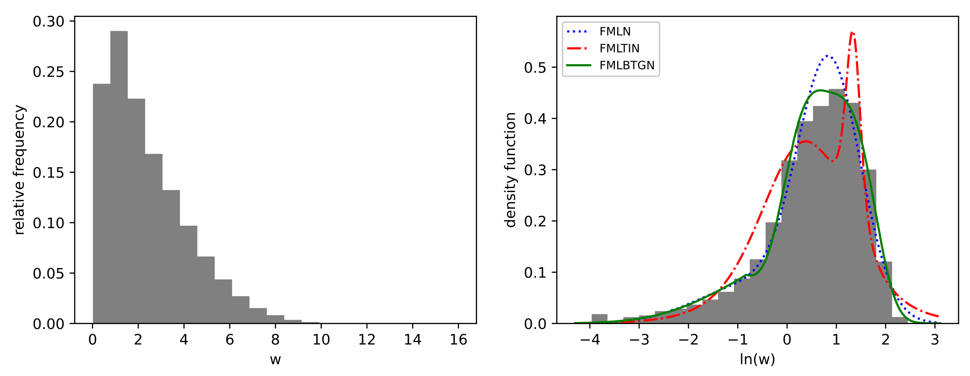
The in-sample criterion, average , and average fitted fold estimates are tabulated in Table 5. The and (divided by n for easier comparison) are the lowest for the FMLBTGN, and the is the highest for the FMLBTGN. It can therefore be concluded that the FMLBTGN model fits best. Visually comparing the fitted density functions shown in Figure 10, the FMLBTGN confirms the latter conclusion by providing the closest fit. The FMLTIN performed the worst of the finite mixtures with the lowest and visual fit to the data. The FMLTIN has two drawbacks compared to the FMLBTGN; it can only inflate the tail of the distribution and not deflate, and it cannot separately control the body shape of the distribution. The location, scale, and mixing proportions of the FMLN are very similar to those of the FMLBTGN, showing that the FMLBTGN mostly adjusted body and tail shapes to fit the data. Focusing on FMLBTGN, the first component has a “sharper” than normal body and lighter than normal tails of . The second component has a “flatter” body shape and lighter than normal tails , respectively.
Table 5.
Fitted two-component mixture distributions, in-sample criterion, and cross-validated LL.
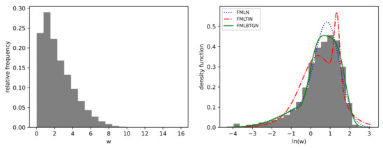
Figure 10.
Histogram of hourly wind speed measurements and fitted finite mixture density functions.
The main shortcoming of the FMLBTGN fit is that the log wind data are skewed more than the mixture can account for. This is evident with the mode of the FMLBTGN not matching the mode of the histogram. The addition of a skewness parameter would complement the analysis by taking into account and highlighting the fundamental skew nature of the skew log-wind speed data tying back to the desirable traits, as outlined in Section 1.
7.5. Application Conclusion
The body and tail parameters of the BTGN have enhanced the capability of the normal distribution to fit the data better in these three different data modeling situations. From the overall results, it can be concluded that BTGN demonstrates a practical benefit to portfolio selection, time series analysis, and finite component mixtures.
8. Conclusions
This paper outlines and motivates the derivative kernel integration method for generating distributions, while generalizing the normal and GN distributions. This method produced an intuitive body-tail generalization of the normal distribution, with the following desirable traits:
- a closed-form density function unlike the ASSG distribution (excluding the Cauchy distribution);
- a single parameter governing body and tail shape unlike the majority of distributions nested in the symmetric GHYP distribution;
- finite moments regardless of shape parameter selection differently from the t and ASSG distributions;
- light and heavy-tailed kurtosis is achievable, unlike the TIN, GN, and t distributions;
- possess simple equations and tractability.
Derivations of important statistical quantities and equations are provided, such as the density function, CDF, moments, MGF, ML, and MPS. Finally, the new properties of the distribution are put to use on log-returns, time series, and finite mixture modeling data, where the BTGN provides a valid alternative to popular distributions. The main possibilities for future work include extending the BTGN to multivariate dimensions, an addition of a skewness parameter, and tests for normality.
Author Contributions
Conceptualization, M.W., A.B. and M.A.; methodology, M.W., A.B. and M.A.; validation, M.W., A.B., M.A.; formal analysis, M.W.; investigation, M.W.; writing-original draft preparation, M.W.; writing—review and editing, A.B., M.A.; visualization, M.W., A.B., M.A.; supervision, A.B., M.A.; project administration, A.B., M.A.; funding acquisition, M.W., A.B., M.A. All authors have read and agreed to the published version of the manuscript.
Funding
This research was funded by the National Research Foundation (NRF) of South Africa, Reference: SRUG190308422768 Grant No. 120839; SARChI Research Chair UID: 71199; Reference: IFR170227223754 Grant No. 109214; the University of Pretoria Visiting Professor Programme; and the Ferdowsi University of Mashhad Grant (N.2/55660).
Institutional Review Board Statement
Not applicable.
Informed Consent Statement
Not applicable.
Data Availability Statement
Not applicable.
Acknowledgments
The authors would like to sincerely thank two reviewers for their constructive comments, which substantially improved the presentation and led us to add many details to the paper. Opinions expressed and conclusions arrived at are those of the author and are not necessarily to be attributed to the NRF, University of Pretoria, or the Ferdowsi University of Mashhad.
Conflicts of Interest
The authors declare no conflict of interest.
Appendix A. Lemmas for Derivation of Statistical Quantities
Lemma A1.
Let , then the following limit holds true below:
Proof.
If both factors on the left-hand side of (A1) tend to zero as x tends to infinity. If , by L’Hospital rule
□
Lemma A2.
Let , then the following integral identity holds true
Proof.
Let , which implies . Integrating by parts, where and . The latter implies that and . The integral is evaluated as
Noting from Lemma A1 that the result follows. □
Appendix B. Derivatives for Estimation
The derivatives of the LL function with respect to individual terms inside the sum of (17) are given below:
where , is the digamma function ([32], p. 902), and the Meijer’s G-function ([32], p. 850).
The derivatives of CDF with respect to individual terms for use inside the sum of (20) are given below:
where , and the Meijer’s G-function ([32], p. 850).
Appendix C. Modified Expectation Maximization Algorithm
| Algorithm A1 Modified EM algorithm for k component FMBTGN |
|
References
- De Vries, H. Ueber halbe Galton-Curven als Zeichen discontinuirlicher Variation; Gebrüder Borntraeger: Berlin, Germany, 1894. [Google Scholar]
- McLachlan, G.J.; Lee, S.X.; Rathnayake, S.I. Finite Mixture Models. Annu. Rev. Stat. Appl. 2000, 6, 355–378. [Google Scholar] [CrossRef]
- Barndorff-Nielsen, O.; Kent, J.; Sørensen, M. Normal Variance-Mean Mixtures and z Distributions. Int. Stat. Rev. Rev. Int. Stat. 1982, 50, 145–159. [Google Scholar] [CrossRef]
- Nelsen, R.B. An Introduction to Copulas; Springer: New York, NY, USA, 2007. [Google Scholar]
- Box, G.P.; Cox, D. An analysis of transformations. J. R. Stat. Soc. 1964, 26, 1–43. [Google Scholar] [CrossRef]
- Jones, M. Families of Distributions Arising from Distributions of Order Statistics. Test 2004, 13, 1–43. [Google Scholar] [CrossRef]
- Ferreira, J.; Steel, M. A constructive Representation of Univariate Skewed Distributions. J. Am. Stat. Assoc. 2006, 101, 823–829. [Google Scholar] [CrossRef] [Green Version]
- Pearson, K. Memoir on skew variation in homogenous material. Philos. Trans. R. Soc. A 1895, 186, 343–414. [Google Scholar]
- Hansen, B.E. Autoregressive Conditional Density Estimation. Int. Econ. Rev. 1994, 35, 705–730. [Google Scholar] [CrossRef]
- Naveau, P.; GeGenton, M.; Shen, X. A skewed Kalman filter. J. Multivar. Anal. 2005, 94, 382–400. [Google Scholar] [CrossRef] [Green Version]
- Allard, D.; Naveau, P. A New Spatial Skew-Normal Random Field Model. Commun. Stat.-Theory Methods 2007, 36, 1821–1834. [Google Scholar] [CrossRef]
- Azzalini, A.; Genton, M. Robust Likelihood Methods Based on the Skew-t and Related Distributions. Int. Stat. Rev. 2008, 76, 106–129. [Google Scholar] [CrossRef]
- Arellano-Valle, R.; Bolfarine, H.; Lachos, V. Skew-normal linear mixed models. J. Data Sci. 2005, 3, 415–438. [Google Scholar] [CrossRef]
- Pereira, M.A.A.; Russo, C.M. Nonlinear mixed-effects models with scale mixture of skew-normal distributions. J. Appl. Stat. 2019, 46, 1602–1620. [Google Scholar] [CrossRef]
- Rubio, F.J.; Steel, M. Inference in Two-piece Location-Scale Models with Jeffreys priors. Bayesian Anal. 2014, 9, 1–22. [Google Scholar] [CrossRef]
- Maleki, M.; Wraith, D.; AArellano-Valle, R.B. A flexible class of parametric distributions for Bayesian linear mixed models. Test 2018, 28, 1–22. [Google Scholar] [CrossRef]
- Ley, C. Flexible modeling in statistics: Past, present and future. J. Soc. Fr. Stat. 2015, 156, 76–96. [Google Scholar]
- Jones, M. On Families of Distributions with Shape Parameters. Int. Stat. Rev. 2015, 83, 175–192. [Google Scholar] [CrossRef]
- McLeish, D.L. A Robust Alternative to the Normal Distribution. Can. J. Stat. Rev. Can. Stat. 1982, 10, 89–102. [Google Scholar] [CrossRef] [Green Version]
- Azzalini, A. A class of distributions which includes the normal ones. Scand. J. Stat. 1985, 12, 171–178. [Google Scholar]
- Johnson, N.L. Systems of Frequency Curves Generated by Methods of Translation. Biometrika 1949, 36, 149–176. [Google Scholar] [CrossRef] [PubMed]
- Tukey, J.W. Modern techniques in data analysis. In Proceedings of the NSF-Sponsored Regional Research Conference; Southeastern Massachusetts University: North Dartmouth, MA, USA, 1977; Volume 7. [Google Scholar]
- Rieck, J.R.; Nedelman, J.R. A Log-Linear Model for the BirnbaumSaunders Distribution. Technometrics 1991, 33, 51–60. [Google Scholar]
- Jones, M.; Pewsey, A. Sinh-arcsinh distributions. Biometrika 2009, 96, 761–780. [Google Scholar] [CrossRef] [Green Version]
- Subbotin, M.T. On the Law of Frequency of Error. Mathematicheskii Sbornik 1923, 31, 296–301. [Google Scholar]
- Box, G.E.; Tiao, G. A further look at robustness via Bayes’s theorem. Biometrika 1962, 49, 419–432. [Google Scholar] [CrossRef]
- Box, G.E.; Tiao, G.C. Bayesian Inference in Statistical Analysis; Addison Wesley: Boston, MA, USA, 1973; Volume 1. [Google Scholar]
- Arashi, M.; Nadarajah, S. Generalized elliptical distributions. Commun. Stat.-Theory Methods 2017, 46, 6412–6432. [Google Scholar] [CrossRef]
- Nadarajah, S.; Teimouri, M. On the Characteristic Function for Asymmetric Exponential Power Distributions. Econom. Rev. 2012, 31, 475–481. [Google Scholar] [CrossRef]
- Johnson, N.; Kotz, S.; Balakrishnan, N. Continuous Univariate Distributions; John Wiley & Sons: Hoboken, NJ, USA, 1994; Volume 2. [Google Scholar]
- Barndorff-Nielsen, O. Hyperbolic Distributions and Distributions on Hyperbolae. Scand. J. Stat. 1978, 5, 151–157. [Google Scholar]
- Gradshteyn, I.; Ryhzhik, I. Table of Integrals, Series and Products; Academic Press: Cambridge, MA, USA, 2007. [Google Scholar]
- Scott, D.J.; Würtz, D.; Dong, C.; Tran, T.T. Moments of the generalized hyperbolic distribution. Comput. Stat. 2011, 26, 459–476. [Google Scholar] [CrossRef] [Green Version]
- Cheng, R.; Stephens, M. A goodness-of-fit test using Moran’s statistic with estimated parameters. Biometrika 1989, 76, 385–392. [Google Scholar] [CrossRef]
- Cheng, R.; Amin, N. Estimating Parameters in Continuous Univariate Distributions with a Shifted Origin. J. R. Stat. Soc. Ser. B 1983, 45, 394–403. [Google Scholar] [CrossRef]
- Ranneby, B. The Maximum Spacing Method. An Estimation Method Related to the Maximum Likelihood Method. Scand. J. Stat. 1984, 11, 93–112. [Google Scholar]
- Dempster, A.P.; Laird, N.M.; Rubin, D.B. Maximum likelihood from incomplete data via the EM algorithm. J. R. Stat. Soc. Ser. B. 1977, 39, 1–22. [Google Scholar]
- Blume, M. Expectation Maximization: A Gentle Introduction; Technical University of Munich Institute for Computer Science: Munich, Germany, 2002. [Google Scholar]
- McLachlan, G.J.; Krishnan, T. The EM Algorithm and Extensions; John Wiley & Sons: Hoboken, NJ, USA, 2007; Volume 382. [Google Scholar]
- Biernacki, C.; Celeux, G.; Govaert, G. Choosing starting values for the EM algorithm for getting the highest likelihood in multivariate Gaussian mixture models. Comput. Stat. Data Anal. 2003, 41, 561–575. [Google Scholar] [CrossRef]
- Box, G.E.P.; Jenkins, G.M.; Reinsel, G.C.; Ljung, G. Time Series Analysis: Forecasting and Control; John Wiley & Sons: Hoboken, NJ, USA, 2015. [Google Scholar]
- Harris, C.R.; Millman, K.J.; van der Walt, S.J.; Gommers, R.; Virtanen, P.; Cournapeau, D.; Wieser, E.; Taylor, J.; Berg, S.; Smith, N.J.; et al. Array programming with NumPy. Nature 2020, 585, 357–362. [Google Scholar] [CrossRef] [PubMed]
- Virtanen, P.; Gommers, R.; Oliphant, T.E.; Haberland, M.; Reddy, T.; Cournapeau, D.; Burovski, E.; Peterson, P.; Weckesser, W.; Bright, J.; et al. SciPy 1.0: Fundamental Algorithms for Scientific Computing in Python. Nat. Methods 2020, 17, 261–272. [Google Scholar] [CrossRef] [Green Version]
- Johansson, F. mpmath: A Python Library for Arbitrary-Precision Floating-Point Arithmetic (Version 1.1.0). 2018. Available online: http://mpmath.org/ (accessed on 20 August 2021).
- Fama, E.F. Portfolio Analysis in a Stable Paretian Market. Manag. Sci. 1965, 11, 404–419. [Google Scholar] [CrossRef]
- Mandelbrot, B.B. The Variation of Certain Speculative Prices. In Fractals and Scaling in Finance; Springer: Berlin/Heidelberg, Germany, 1997; pp. 371–418. [Google Scholar]
- Bingham, N.H.; Kiesel, R. Semi-parametric modeling in finance: Theoretical foundations. Quant. Financ. 2002, 2, 241. [Google Scholar] [CrossRef]
- McNeil, A.J.; Frey, R.; Embrechts, P. Quantitative Risk Management: Concepts, Techniques and Tools Revised Edition. In Economics Books; Princeton University Press: Princeton, NJ, USA, 2015. [Google Scholar]
- Kring, S.; Rachev, S.T.; Höchstötter, M.; Fabozzi, F.J. Estimation of α-stable sub-Gaussian Distributions for Asset Returns. In Risk Assessment; Springer: Berlin/Heidelberg, Germany, 2009; pp. 111–152. [Google Scholar]
- Behr, A.; Pötter, U. Alternatives to the normal model of stock returns: Gaussian mixture, generalised logF and generalised hyperbolic models. Ann. Financ. 2009, 5, 49–68. [Google Scholar] [CrossRef]
- Rachev, S.T.; Hoechstoetter, M.; Fabozzi, F.J.; Focardi, S.M. Probability and Statistics for Finance; John Wiley & Sons: Hoboken, NJ, USA, 2010; Volume 176. [Google Scholar]
- Prause, K. The Generalized Hyperbolic Model: Estimation, Financial Derivatives, and Risk Measures. Ph.D. Thesis, Albert-Ludwigs-Universitat Freiburg, Freiburg im Breisgau, Germany, 1999. [Google Scholar]
- Weibel, M.; Luethi, D.; Breymann, W. ghyp: Generalized Hyperbolic Distribution and Its Special Cases (Version 1.6.1). 2020. Available online: https://cran.r-project.org/web/packages/ghyp (accessed on 20 August 2021).
- Petroleum, B. BP Statistical Review of World Energy 2021. British Petroleum. 2021. Available online: https://www.bp.com/en/global/corporate/energy-economics/statistical-review-of-world-energy.html (accessed on 20 August 2021).
- Burton, T.; Sharpe, D.; Jenkins, N.; Bossanyi, E. Wind Energy Handbook; John Wiley & Sons: Hoboken, NJ, USA, 2001; Volume 2. [Google Scholar]
- Akpinar, S.; Akpinar, E.K. Estimation of wind energy potential using finite mixture distribution models. Energy Convers. Manag. 2009, 50, 877–884. [Google Scholar] [CrossRef]
- Punzo, A.; Bagnato, L. The multivariate tail-inflated normal distribution and its application in finance. J. Stat. Comput. Simul. 2021, 91, 1–36. [Google Scholar] [CrossRef]


Publisher’s Note: MDPI stays neutral with regard to jurisdictional claims in published maps and institutional affiliations. |
© 2021 by the authors. Licensee MDPI, Basel, Switzerland. This article is an open access article distributed under the terms and conditions of the Creative Commons Attribution (CC BY) license (https://creativecommons.org/licenses/by/4.0/).