Approximate Solutions for a Class of Nonlinear Fredholm and Volterra Integro-Differential Equations Using the Polynomial Least Squares Method

Abstract

We apply the polynomial least squares method to obtain approximate analytical solutions for a very general class of nonlinear Fredholm and Volterra integro-differential equations. The method is a relatively simple and straightforward one, but its precision for this type of equations is very high, a fact that is illustrated by the numerical examples presented. The comparison with previous approximations computed for the included test problems emphasizes the method’s simplicity and accuracy.

1. Introduction

Integro-differential equations are important in both pure and applied mathematics, with multiple applications in mechanics, engineering, physics, etc. The behavior and evolution of many physical systems in many fields of science and engineering, including, for example, visco-elasticity, evolutionary problems, fluid dynamics, the dynamics of populations and many others, may be successfully modeled by using integro-differential equations of the Fredholm or Volterra type.

The beginning of the theory of integral equations can be attributed to N. H. Abel (1802–1829), who formulated an integral equation in 1812 by studying a problem of mechanics. Since then, many other great mathematicians, including T. Lalescu (who wrote the world’s first dissertation of integral equations in 1911), A. Cauchy (1789–1857), J. Liouville (1809–1882), V. Volterra (1860–1940), I. Fredholm (1866–1927), D. Hilbert (1862–1943), and E. Picard (1856–1941) have contributed to the field of integral and integro-differential equations. In the 20th century, the theory of integral equations presented a strong development regarding both the perspective of its applications and the actual methods of computation of the solutions. Among the main methods used in the study of integral and integro-differential equations, we mention fixed point methods, variational methods, iterative methods, numerical methods and approximate methods.

The class of equations studied in this paper has the following general expression:

$$\begin{array}{r}{\displaystyle \sum _{j=0}^n}{p}_j\left(x\right)\times u^{\left(j\right)}\left(x\right)=f\left(x\right)+{\lambda }_1\times \underset{a}{\overset{x}{\int }}{k}_1(x,s)\times g_1(s,u\left(s\right),u^{\prime }\left(s\right))ds\\ +{\lambda }_2\times \underset{a}{\overset{b}{\int }}{k}_2(x,s)\times g_2(s,u\left(s\right),u^{\prime }\left(s\right))ds,\end{array}$$

(1)

and, depending on the problem, may have attached a set of boundary conditions of the following type:

$$\sum _{j=0}^{n-1}\left[{\alpha }_{ij}\times u^{\left(j\right)}\left(a\right)+{\beta }_{ij}\times u^{\left(j\right)}\left(b\right)\right]={\mu }_i,i=0,\dots ,n-1.$$

(2)

Here, $a,b,{\lambda }_1,{\lambda }_2$ are constants and we assume that the functions $p_j(j=0,\dots ,n)$, f, $k_1$, $k_2$, $g_1$, $g_2$ have suitable derivatives on $[a,b]$ such that the problem consisting of Equation (1) together with the set of conditions of (2) (if present) admits a solution.

We remark that this class of equations evidently includes both Fredholm- and Volterra-type equations, linear and nonlinear equations and, also, both integro-differential and integral equations, so it is a very general class of equations indeed.

While the qualitative properties of integro-differential equations are thoroughly studied ([1,2]), leaving aside a relatively small number of exceptions (mostly test problems, such as the ones included as examples), the exact solution of a nonlinear integro-differential equation of the type (1) cannot be found, and numerical solutions or approximate analytical solutions must be computed. Of these two types of solutions, the approximate analytical ones are usually more useful if any subsequent computation involving the solution must be performed.

Of course, many approximation techniques have been proposed for the computation of analytic approximations of integro-differential Fredholm and Volterra equations, such as, for example, the following: Taylor expansion methods ([3,4]), Tau methods ([5,6]), the homotopy perturbation method ([7]), the Bessel polynomials method ([8]), Legendre methods ([9]), the Bernoulli matrix method ([10]), the Haar wavelet method ([11,12,13]), collocation methods ([14,15]), the Bernstein–Kantorovich operators method ([16]), Cattani’s method ([17]), the variational iteration method ([18]), the Bernstein polynomials-based projection method ([19]), the block pulse functions method ([20,21,22]), the modified decomposition method ([23]), and the differential transform method ([24]).

2. The Polynomial Least Squares Method

We associate to the problem (1) and (2) the following operator:

$$\begin{array}{r}D\left(u\right)={\displaystyle \sum _{j=0}^n}{p}_j\left(x\right)\times u^{\left(j\right)}\left(x\right)-f\left(x\right)-{\lambda }_1\times \underset{a}{\overset{x}{\int }}{k}_1(x,s)\times g_1(s,u\left(s\right),u^{\prime }\left(s\right))ds\\ -{\lambda }_2\times \underset{a}{\overset{b}{\int }}{k}_2(x,s)\times g_2(s,u\left(s\right),u^{\prime }\left(s\right))ds.\end{array}$$

(3)

Let $u_{app}$ denote an approximate solution of (1). If we replace the exact solution u of (1) with $u_{app}$, then the error corresponding to this replacement can be described by the so-called remainder:

$$R(x,u_{app})=D\left(u_{app}\left(x\right)\right),x\in [a,b].$$

(4)

We find approximate polynomial solutions $u_{app}$ of (1) and (2) on $[a,b]$ such that $u_{app}$ satisfies the following conditions:

$$\left|R\right(x,u_{app}\left)\right|<\epsilon ,$$

(5)

$$\sum _{j=0}^{n-1}\left[{\alpha }_{ij}\times u_{app}^{\left(j\right)}\left(a\right)+{\beta }_{ij}\times u_{app}^{\left(j\right)}\left(b\right)\right]={\mu }_i,i=0,\dots ,n-1.$$

(6)

Definition 1.

An approximate polynomial solution $u_{app}$, which satisfies the relations (5) and (6), is called a ε-approximate polynomial solution of the problem (1) and (2).

Definition 2.

An approximate polynomial solution $u_{app}$ satisfying the relation $\underset{a}{\overset{b}{\int }}{R}^2(x,u_{app})\mathit{dx}\le$ δ together with the initial conditions (6), is called a weak δ-approximate polynomial solution of the problem (1) and (2).

Definition 3.

Let there be the sequence of polynomials $P_m\left(x\right)=a_0+a_{1}x+\dots +a_m{x}^m$, $a_i\in \mathbb{R}$, $i=0,1,\dots ,m$ which satisfy the following conditions:

$$\sum _{j=0}^{n-1}\left[{\alpha }_{ij}\times P_m^{\left(j\right)}\left(a\right)+{\beta }_{ij}\times P_m^{\left(j\right)}\left(b\right)\right]={\mu }_i,i=0,\dots ,n-1.$$

The sequence of polynomials $P_m\left(x\right)$ is called convergent to the solution of the problem (1) and (2) if $\underset{m\to \infty }{lim}D\left(P_m\left(x\right)\right)=0$.

We can prove the following theorem regarding the convergence of the method.

Theorem 1.

If $T_m\left(x\right)$ denotes a weak ε-approximate polynomial solution of the problem (1) and (2), then the necessary condition for the problem to admit a sequence of polynomials $P_m\left(x\right)$ convergent to its solution is as follows: $\underset{m\to \infty }{lim}\underset{a}{\overset{b}{\int }}{R}^2(x,T_m)\mathit{dx}=0.$

Proof. 

We compute a weak $\epsilon$-polynomial solution:

$$\tilde{u}\left(x\right)=\sum _{k=0}^m{c}_k\times x^k,m>n.$$

(7)

The constants $c_0,c_1,\dots ,c_m$ are determined by performing the computations included in the following steps:

• First, we replace the approximate solution (7) in the Equation (1), obtaining the following expression:

  $$\begin{array}{c}{\displaystyle \mathit{R}(x,c_0,c_1,\dots ,c_m)=R(x,\tilde{u})=\sum _{j=0}^n{p}_j\left(x\right)\times {\tilde{u}}^{\left(j\right)}\left(x\right)-f\left(x\right)}\\ -{\lambda }_1\times \underset{a}{\overset{x}{\int }}{k}_1(x,s)\times g_1(s,\tilde{u}\left(s\right),{\tilde{u}}^{\prime }\left(s\right))ds-{\lambda }_2\times \underset{a}{\overset{b}{\int }}{k}_2(x,s)\times g_2(s,\tilde{u}\left(s\right),{\tilde{u}}^{\prime }\left(s\right))ds.\end{array}$$

  (8)
  If we could find the constants $c_0^0,c_1^0,\dots ,c_m^0$ such that $\mathit{R}(x,c_0^0,c_1^0,\dots ,c_m^0)=0$ $\forall x\in [a,b]$ and if the corresponding expressions of (2) (if included in the problem)

  $$\sum _{j=0}^{n-1}\left[{\alpha }_{ij}\times {\tilde{u}}^{\left(j\right)}\left(a\right)+{\beta }_{ij}\times {\tilde{u}}^{\left(j\right)}\left(b\right)\right]={\mu }_i,i=0,\dots ,n-1$$

  (9)

  are also satisfied, then by substituting $c_0^0,c_1^0,\dots ,c_m^0$ in (7), we find the exact solution of (1) and (2).
• Next, we associate to (1) and (2) the following functional:

  $$J(c_n,c_{n+1},\dots ,c_m)=\underset{a}{\overset{b}{\int }}{\mathit{R}}^2(x,c_0,c_1,\dots ,c_m)\mathit{dx}$$

  (10)

  where $c_0,c_1,\dots ,c_{n-1}$ may be determined as functions of $c_n,c_{n+1},\dots ,c_m$ by means of the conditions (9) (if such conditions are included). If the conditions are not included, then J is simply a function of $c_0,c_1,\dots ,c_m$ (as in the case of our last example).
• If the conditions are included, we compute $c_n^0,c_{n+1}^0,\dots ,c_m^0$ as the values corresponding to the minimum of the functional (10) and $c_0^0,c_1^0,\dots ,c_{n-1}^0$ again as functions of $c_n^0,c_{n+1}^0,\dots ,c_m^0$ by using the initial conditions. If the conditions are not included, then $c_0^0,c_1^0,\dots ,c_m^0$ are the values that correspond to the minimum of the functional.
• Using $c_0^0,c_1^0,\dots ,c_m^0$ computed at the previous step, we construct the following polynomial:

  $$T_m\left(x\right)=\sum _{k=0}^m{c}_k^0{x}^k.$$

  (11)

Considering the relations (8)–(11) and the way the coefficients of $T_m\left(x\right)$ are computed, it can be deduced that the following inequality holds:

$$0\le \underset{a}{\overset{b}{\int }}{R}^2(x,T_m\left(x\right))\mathit{dx}\le \underset{a}{\overset{b}{\int }}{R}^2(x,P_m\left(x\right))\mathit{dx},\forall m\in \mathbb{N}.$$

Hence,

$$0\le \underset{m\to \infty }{lim}\underset{a}{\overset{b}{\int }}{R}^2(x,T_m\left(x\right))\mathit{dx}\le \underset{m\to \infty }{lim}\underset{a}{\overset{b}{\int }}{R}^2(x,P_m\left(x\right))\mathit{dx}=0.$$

Thus,

$$\underset{m\to \infty }{lim}\underset{a}{\overset{b}{\int }}{R}^2(x,T_m\left(x\right))\mathit{dx}=0.$$

From the above limit, we deduce that $\forall \epsilon >0,\exists m_0\in \mathbb{N}$ such that $\forall m\in \mathbb{N},m>m_0$, it follows that $T_m\left(x\right)$ is a weak $\epsilon$-approximate polynomial solution of (1) and (2). □

Remark 1.

We observe that if ${\tilde{u}}_{app}$ is a ε-approximate polynomial solution of (1) and (2), then ${\tilde{u}}_{app}$ is also a weak ${\epsilon }^2\times (b-a)$-approximate polynomial solution. However, the reciprocal property is not always true. As a consequence, we deduce that the set of weak approximate solutions of (1) and (2) contains also the approximate solutions of the problem.

As a consequence of the previous Remark, in order to compute $\epsilon$-approximate polynomial solutions of the problem (1) and (2) by the polynomial least squares method (from now on denoted as PLSM), we first compute the weak approximate polynomial solutions, ${\tilde{u}}_{app}$. If $\left|R\right(t,{\tilde{u}}_{app}\left)\right|<\epsilon$, then ${\tilde{u}}_{app}$ is also a $\epsilon$-approximate polynomial solution of the problem.

Remark 2.

Regarding the practical implementation of the method, we wish to make the following remarks:

• Regarding the choice of the degree of the polynomial approximation, in the computations, we usually start with the lowest degree (i.e., first degree polynomial) and compute successively higher degree approximations until the error (see next item) is considered low enough from a practical point of view for the given problem (or, in the case of a test problem, until the error is lower than the error corresponding to the solutions obtained by other methods). Of course, in the case of a test problem when the known solution is a polynomial, one may start directly with the corresponding degree, but this is just a shortcut and by no means necessary when using the method.
• If the exact solutions of the problem are not known, as would be the case of a real-life problem, and as a consequence, the error cannot be computed, then instead of the actual error, we can consider as an estimation of the error the value of the remainder R (4) corresponding to the computed approximation, as mentioned in the previous remark.
• If the problem has an (unknown) exact polynomial solution, it is easy to see if PLSM has found it since the value of the minimum of the functional in this case is actually 0. In this situation, if we keep increasing the degree (even though there is no point in that), from the computation, we obtain that the coefficients of the higher degrees are actually zero.
• Regarding the choice of the optimization method used for the computation of the minimum of the functional (9), if the solution of the problem is a known polynomial (such as in the case of Application 1, Application 3, Application 5 and Application 6) we usually employ the critical (stationary) points method, because in this way, by using PLSM, we can easily find the exact solution. Such problems are relatively simple ones; the expression of the functional (9) is also not very complicated; and indeed, the solutions can usually be computed even by hand (as in the case of this application). In general, no concerns of conditioning or stability arise.
  However, for a more complicated (real-life) problem, when the solution is not known (or even if the exact solution is known but not polynomial), we would not use the critical points method. In fact, we would not even use a iterative-type method, but rather a heuristic algorithm, such as differential evolution or simulated annealing. In our experience, with this type of problem, even a simple Nelder–Mead-type algorithm works well (as was the case for the following Application 2, Application 4 and Application 7). In fact, Application 4 includes a small comparison of several optimization methods.
• Finally, we remark that in the case when the solution of the problem is not analytic, the convergence of the PLSM solutions will be slower; another basis of functions (wavelets, and piecewise polynomials) should be used to control the approximation levels.

3. Numerical Examples

In this section, we apply PLSM to several well-known test problems, and we compare the solutions obtained by using PLSM with solutions previously computed by means of other methods.

The computations are performed using the Wolfram Mathematica software.

3.1. Application 1: First Order Nonlinear Fredholm Integro-Differential Equation

The first application is an an initial-value problem, including a first-order nonlinear Fredholm integro-differential equation ([7]):

$$\begin{array}{c}{u}^{\prime }\left(x\right)=1-e^{-1}+\underset{0}{\overset{1}{\int }}{e}^{-u^{\prime }\left(s\right)}ds,\\ u\left(0\right)=0.\end{array}$$

(12)

The problem (12) has the exact solution $u_e=x$. As the solution is a polynomial, we expect PLSM to be able to compute this exact solution.

Choosing a first order polynomial, $\tilde{u}\left(x\right)=c_1\times x+c_0$, from the initial condition, it follows that $c_0=0$, so $\tilde{u}\left(x\right)=c_1\times x$.

The corresponding remainder (4) is as follows:

$$\mathit{R}(x,c_1)=R(x,\tilde{u}\left(x\right))=c_1-e^{-c_1}+\frac{1}{e}-1$$

and the corresponding functional (10) is as follows:

$J\left(c_1\right)=\underset{0}{\overset{1}{\int }}{\mathit{R}}^2(x,c_1)\mathit{dx}=2e^{-2c_1-1}\times \left(e^{c_1}+1\right)\times \left(e^{c_1}\times (e\times (c_1-1)+1)-e\right)$.

It is easy to show that the stationary point is $c_1=1$, and this is indeed a minimum of the functional.

We conclude that, as expected, PLSM can find the exact solution of (12).

3.2. Application 2: Second Order Fredholm Integro-Differential Equation

The second application is a problem including a linear second order Fredholm integro-differential equation ([5]):

$$\begin{gathered} u^{″}\left(x\right)=u\left(x\right)-{\displaystyle \frac{4}{\pi }}\underset{0}{\overset{\pi }{\int }}u\left(s\right)cos(x-s)ds, \\ u\left(0\right)=1,u^{\prime }\left(\pi \right)=0. \end{gathered}$$

(13)

The problem (13) has the exact solution $u_e\left(x\right)=cos\left(x\right)$.

Choosing a fifth degree polynomial of the following type,

$$\tilde{u}\left(x\right)=c_0+c_1\times x+c_2\times x^2+c_3\times x^3+c_4\times x^4+c_5\times x^5$$

from the initial conditions, it follows that $c_0=1$ and $c_1=-2\pi c_2-3{\pi }^2{c}_3-4{\pi }^3{c}_4-5{\pi }^4{c}_5$.

Replacing $c_0$ and $c_1$ in $\tilde{u}\left(x\right)$ we compute the remainder (8) as follows:

$\begin{array}{c}\mathit{R}(x,c_2,c_3,c_4,c_5)=R(x,\tilde{u}\left(x\right))={\displaystyle \frac{1}{\pi }}(c_2(-x^2+2\pi x+2)-x^3(c_3-20c_5)+3(2+{\pi }^2)c_{3}x+\hfill \\ +{\pi }^{3}x(4c_4+5\pi c_5)-c_4{x}^4+12c_4{x}^2-c_5{x}^5-1)-4sin\left(x\right)((4+{\pi }^2)c_2+6\pi (c_3-20c_5)+\hfill \\ +2{\pi }^3(c_3+2(5+{\pi }^2)c_5)+3(-16+4{\pi }^2+{\pi }^4)c_4-2)+4cos\left(x\right)(2\pi (c_2+2(6+{\pi }^2)c_4)+\hfill \\ +3(4+{\pi }^2)c_3+5(-48+12{\pi }^2+{\pi }^4)c_3).\hfill \end{array}$

We minimize the corresponding functional $\mathit{J}(c_2,c_3,c_4,c_5)$ (10) (whose expression is too large to be presented), and the corresponding values of the constants are as follows:

$$c_2=-0.495256234419017,c_3=-0.014423630344293588,$$

$$c_4=0.0570671588506153,c_5=-0.00726601260392728.$$

We compute $c_0$ and $c_1$ by using again the initial conditions obtaining the approximation:

$$\begin{array}{c}\tilde{u}\left(x\right)=-0.007266012603927289\times x^5+0.0570671588506153\times x^4\\ -0.014423630344293588\times x^3-0.495256234419017\times x^2-0.000028778804548323933\times x+1.\end{array}$$

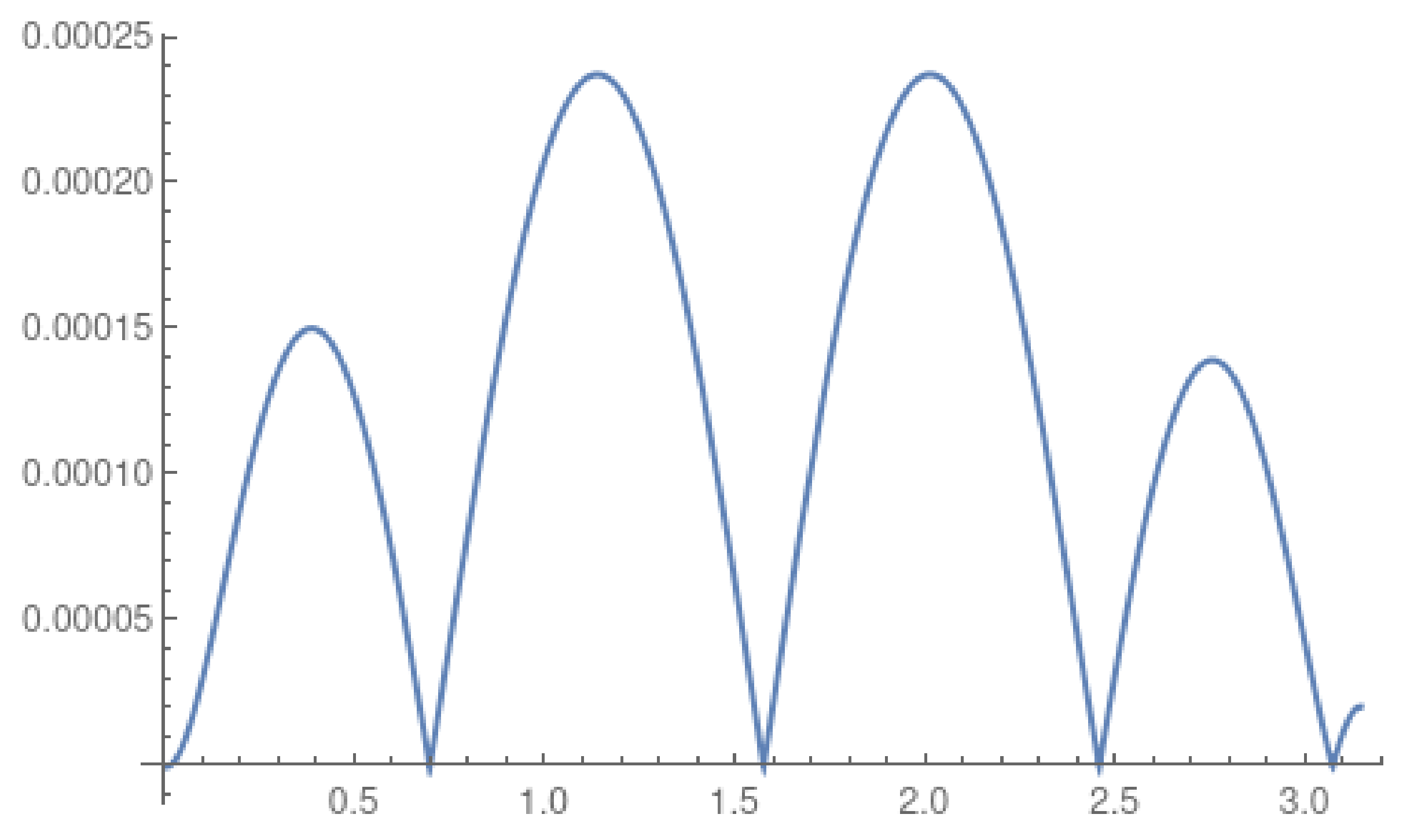
Figure 1 shows the plot of the absolute error corresponding to the above approximation (as the difference in absolute value between the exact solution and the approximation):

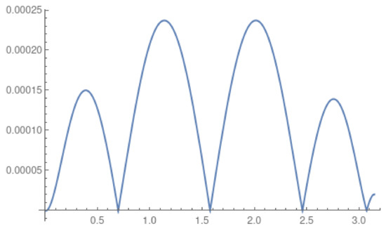
Figure 1. The absolute error of the 5th degree approximation by PLSM for problem (13).

In the same manner, we compute the polynomial approximate solutions of several other degrees, including the following 7th and 9th degree approximations:

• The 7th degree polynomial approximation:

  $$\begin{array}{c}\tilde{u}\left(x\right)=0.00018041589065861824\times x^7-0.0019837763283978385\times x^6\hfill \\ +0.0010565364433122195\times x^5+0.04064970121350719\times x^4\hfill \\ +0.0004810728874007701\times x^3-0.5000823975257741\times x^2\hfill \\ -2.0682771051383497\times {10}^{-9}\times x+1,\hfill \end{array}$$
• The 9th degree polynomial approximation:

  $$\begin{array}{c}\tilde{u}\left(x\right)=-2.562518981850636\times {10}^{-6}\times x^9+0.000036226759498841756\times x^8\hfill \\ -0.000029771048432999026\times x^7-0.0013411879139737842\times x^6\hfill \\ -0.00004669167457397479\times x^5+0.04169310448407386\times x^4\hfill \\ -7.6134363553432504\times {10}^{-6}\times x^3-0.49999919540973176\times x^2\hfill \\ -3.2152058793144533\times {10}^{-13}\times x+1.\hfill \end{array}$$

Table 1 compares the absolute errors of the approximation obtained by using the operational Tau method ([5]) and of the approximations obtained by using PLSM.

Table 1. Absolute errors of the approximations for problem (13).

x	[5]	PLSM 5th	PLSM 7th	PLSM 9th
0	0	0	0	0
0.3	$1.070\times {10}^{-6}$	$1.369\times {10}^{-4}$	$4.933\times {10}^{-7}$	$3.500\times {10}^{-9}$
0.7	$5.452\times {10}^{-6}$	$4.566\times {10}^{-6}$	$1.478\times {10}^{-6}$	$6.276\times {10}^{-9}$
0.99	$3.847\times {10}^{-3}$	$2.056\times {10}^{-4}$	$6.660\times {10}^{-7}$	$3.966\times {10}^{-9}$
1.19	$4.273\times {10}^{-3}$	$2.328\times {10}^{-4}$	$1.932\times {10}^{-6}$	$8.115\times {10}^{-9}$
1.49	$4.591\times {10}^{-3}$	$6.864\times {10}^{-4}$	$7.601\times {10}^{-7}$	$5.214\times {10}^{-9}$
1.97	$7.285\times {10}^{-4}$	$2.352\times {10}^{-4}$	$1.881\times {10}^{-6}$	$7.227\times {10}^{-9}$
2.27	$6.066\times {10}^{-4}$	$1.407\times {10}^{-4}$	$4.163\times {10}^{-7}$	$8.899\times {10}^{-9}$
2.66	$1.771\times {10}^{-3}$	$1.238\times {10}^{-4}$	$8.749\times {10}^{-7}$	$5.308\times {10}^{-9}$
3.06	$3.173\times {10}^{-4}$	$3.749\times {10}^{-6}$	$3.332\times {10}^{-7}$	$2.236\times {10}^{-9}$

We remark that the solution presented in [5] is a piecewise constructed function consisting of 7 polynomials of 5th degree.

As the comparison clearly shows, the PLSM solutions, even though they consist of a single polynomial (and thus, are much easier to work with) offer much better accuracy.

Moreover, Table 1 illustrates the convergence of the method since the error decreases quickly when the degree of the polynomial approximation increases.

3.3. Application 3: Voltera Integro-Differential Equation

We consider a Voltera integro-differential equation together with the initial condition [21]):

$$\begin{array}{c}u\left(x\right)+\underset{0}{\overset{x}{\int }}sin(x-s)u\left(s\right)u^{\prime }\left(s\right)ds=2x^3+x^2-12x+12sin\left(x\right),\\ u\left(0\right)=0.\end{array}$$

(14)

The problem (14) has the exact solution $u_e\left(x\right)=x^2$.

Choosing the approximate solution as a second degree polynomial, $\tilde{u}\left(x\right)=c_2{x}^2+c_{1}x+c_0$ and following the steps described in the PLSM algorithm, the exact solution of the problem is computed.

We remark that the numerical approximation $u_{bp}$ computed in [21] using block-pulse and hybrid functions leads to errors between ${10}^{-4}$ and ${10}^{-6}$.

3.4. Application 4: Nonlinear Volterra Integral Equation

The next application is a nonlinear Volterra integral equation ([11]):

$$u\left(x\right)+\underset{0}{\overset{x}{\int }}(u^2\left(s\right)+u\left(s\right))ds={\displaystyle \frac{3}{2}}-{\displaystyle \frac{1}{2}}{e}^{-2x}.$$

(15)

The problem has the exact solution $u_e=e^{-x}$.

Employing the same PLSM steps used in the previous examples, we calculated several approximate polynomial solutions. Regarding the computation of the minimum of the functional $\mathit{J}$ (10), we wish to make the following remark: As addressed in Remark 2.2, the method of the computation of the minimum is not specified as a part of the PLSM algorithm. In the previous applications, where the exact solutions were polynomial, it seemed natural to use the critical/stationary points method since this way, it is easy to find the exact solution. However, when the solution is not known (or known but not a polynomial), it could be preferable to use other types of optimization algorithms, such as, for example, heuristic algorithms. In the following, we present several approximations obtained by using different optimization algorithms:

• The 7th degree polynomial approximation, using the stationary points method:

  $$\begin{array}{c}{\tilde{u}}_{SP}\left(x\right)=-0.00011345611365715616\times x^7+0.0012464556997988509\times x^6\hfill \\ -0.0082011259042975\times x^5+0.041596100222452324\times x^4\hfill \\ -0.16664543699098286\times x^3+0.4999966895170558\times x^2\hfill \\ -0.9999997806314149\times x+0.9999999964067919.\hfill \end{array}$$
• The 7th degree polynomial approximation, using a differential evolution algorithm:

  $$\begin{array}{c}{\tilde{u}}_{DE}\left(x\right)=-0.00011316054070325334\times x^7+0.0012454011895116283\times x^6\hfill \\ -0.008199632407882492\times x^5+0.04159503453392284\times x^4\hfill \\ -0.16664503638050765\times x^3+0.49999661433923326\times x^2\hfill \\ -0.9999997747534194\times x+0.9999999962937947.\hfill \end{array}$$
• The 7th degree polynomial approximation, using a simulated annealing algorithm:

  $$\begin{array}{c}{\tilde{u}}_{SA}\left(x\right)=-0.00011316266584759397\times x^7+0.0012454096786813414\times x^6\hfill \\ -0.008199645948810286\times x^5+0.04159504549729249\times x^4\hfill \\ -0.16664504110233055\times x^3+0.4999966153676161\times x^2\hfill \\ -0.9999997748484193\times x+0.999999996296008.\hfill \end{array}$$
• The 7th degree polynomial approximation, using a Nelder–Mead algorithm:

  $$\begin{array}{c}{\tilde{u}}_{NM}\left(x\right)=-0.00011322093031151744\times x^7+0.0012456159806820094\times x^6\hfill \\ -0.008199935494443129\times x^5+0.041595249823780635\times x^4\hfill \\ -0.16664511685035832\times x^3+0.4999966293278488\times x^2\hfill \\ -0.9999997759134198\times x+0.9999999963157558.\hfill \end{array}$$

In Table 2, we present the comparison of the absolute errors of these approximations. Since in the case of this problem (and in fact, also in the case of the other test problems studied), the functional $\mathit{J}$ (10) does not have a particularly complicated expression, the influence of the optimization method is not very strong (but it could be significant if the initial problem is a very difficult one).

Table 2. Absolute errors of the 7th degree approximations for problem (15) corresponding to different optimization methods.

x	Stationary Points	Differential Evolution	Simulated Annealing	Nelder–Mead
0	$3.59\times {10}^{-9}$	$3.71\times {10}^{-9}$	$3.70\times {10}^{-9}$	$3.68\times {10}^{-9}$
0.1	$5.99\times {10}^{-10}$	$6.31\times {10}^{-10}$	$6.29\times {10}^{-10}$	$6.24\times {10}^{-10}$
0.2	$9.92\times {10}^{-10}$	$1.02\times {10}^{-9}$	$1.02\times {10}^{-9}$	$1.01\times {10}^{-9}$
0.3	$3.23\times {10}^{-10}$	$3.16\times {10}^{-10}$	$3.17\times {10}^{-10}$	$3.17\times {10}^{-10}$
0.4	$7.06\times {10}^{-10}$	$7.32\times {10}^{-10}$	$7.32\times {10}^{-10}$	$7.26\times {10}^{-10}$
0.5	$2.92\times {10}^{-10}$	$2.86\times {10}^{-10}$	$2.86\times {10}^{-10}$	$2.86\times {10}^{-10}$
0.6	$5.99\times {10}^{-10}$	$6.22\times {10}^{-10}$	$6.22\times {10}^{-10}$	$6.17\times {10}^{-10}$
0.7	$2.49\times {10}^{-10}$	$2.43\times {10}^{-10}$	$2.43\times {10}^{-10}$	$2.44\times {10}^{-10}$
0.8	$4.62\times {10}^{-10}$	$4.86\times {10}^{-10}$	$4.86\times {10}^{-10}$	$4.80\times {10}^{-10}$
0.9	$4.83\times {10}^{-10}$	$4.96\times {10}^{-10}$	$4.97\times {10}^{-10}$	$4.93\times {10}^{-10}$

Using PLSM with the Nelder–Mead algorithm, we compute approximations of different degrees. In the comparison, we use the following approximate solutions:

• The 4th degree polynomial approximation:

  $$\begin{array}{c}\tilde{u}\left(x\right)=0.025564089018833714\times x^4-0.1536250257345637\times x^3\hfill \\ +0.49533159454597286\times x^2-0.9993502611714822\times x+0.9999785976907262,\hfill \end{array}$$
• The 5th degree polynomial approximation:

  $$\begin{array}{c}\tilde{u}\left(x\right)=-0.005103615073120197\times x^5+0.03831931089978327\times x^4\hfill \\ -0.1649623295804923\times x^3+0.49958537488677296\times x^2\hfill \\ -0.9999592285676391\times x+0.9999990375530758,\hfill \end{array}$$
• The 6th degree polynomial approximation:

  $$\begin{array}{c}\tilde{u}\left(x\right)=0.0008493990830576847\times x^6-0.007651380196990966\times x^5\hfill \\ +0.041214310857115605\times x^4-0.16650657021254095\times x^3\hfill \\ +0.49997167809885856\times x^2-0.9999979253765494\times x+0.99999996317233,\hfill \end{array}$$
• The 7th degree polynomial approximation:

  $$\begin{array}{c}\tilde{u}\left(x\right)=-0.00011322093031151744\times x^7+0.0012456159806820094\times x^6\hfill \\ -0.008199935494443129\times x^5+0.041595249823780635\times x^4\hfill \\ -0.16664511685035832\times x^3+0.4999966293278488\times x^2\hfill \\ -0.9999997759134198\times x+0.9999999963157558.\hfill \end{array}$$

Equation (15) was previously solved by employing the hybrid Taylor block-pulse functions method ([20]) and by employing a combination of the Newton–Kantorovich and Haar wavelet methods ([11]).

Table 3 presents the comparison of the best absolute errors corresponding to these methods and to the above approximations computed by PLSM. In Figure 2, we present the absolute errors corresponding to several of the above PLSM approximations.

Table 3. Absolute errors of the approximations for problem (15).

x	[20]	[11]	PLSM 4th	PLSM 5th	PLSM 6th	PLSM 7th
0	0	$7.90\times {10}^{-3}$	$2.14\times {10}^{-5}$	$9.62\times {10}^{-7}$	$3.68\times {10}^{-8}$	$3.68\times {10}^{-9}$
0.1	$8.33\times {10}^{-4}$	$2.33\times {10}^{-4}$	$2.14\times {10}^{-5}$	$3.68\times {10}^{-7}$	$8.57\times {10}^{-9}$	$6.24\times {10}^{-10}$
0.2	$3.75\times {10}^{-4}$	$1.28\times {10}^{-5}$	$2.95\times {10}^{-6}$	$1.67\times {10}^{-7}$	$1.16\times {10}^{-8}$	$1.01\times {10}^{-9}$
0.3	$1.11\times {10}^{-3}$	$4.25\times {10}^{-4}$	$5.66\times {10}^{-6}$	$2.66\times {10}^{-7}$	$7.86\times {10}^{-10}$	$3.17\times {10}^{-10}$
0.4	$3.51\times {10}^{-4}$	$3.46\times {10}^{-7}$	$6.05\times {10}^{-5}$	$8.43\times {10}^{-8}$	$1.03\times {10}^{-8}$	$7.26\times {10}^{-10}$
0.5	$5.80\times {10}^{-4}$	$1.19\times {10}^{-4}$	$3.33\times {10}^{-7}$	$2.85\times {10}^{-7}$	$3.22\times {10}^{-10}$	$2.86\times {10}^{-10}$
0.6	$1.32\times {10}^{-4}$	$7.97\times {10}^{-6}$	$6.27\times {10}^{-6}$	$6.16\times {10}^{-8}$	$1.02\times {10}^{-8}$	$6.17\times {10}^{-10}$
0.7	$1.95\times {10}^{-4}$	$2.41\times {10}^{-4}$	$5.14\times {10}^{-6}$	$2.69\times {10}^{-7}$	$1.77\times {10}^{-10}$	$2.44\times {10}^{-10}$
0.8	$1.73\times {10}^{-4}$	$2.74\times {10}^{-5}$	$3.31\times {10}^{-6}$	$1.45\times {10}^{-7}$	$1.11\times {10}^{-8}$	$4.80\times {10}^{-10}$
0.9	$3.68\times {10}^{-4}$	$2.56\times {10}^{-4}$	$7.75\times {10}^{-6}$	$3.53\times {10}^{-7}$	$8.47\times {10}^{-9}$	$4.93\times {10}^{-10}$

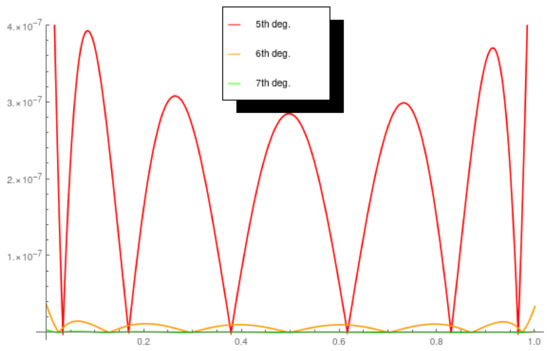
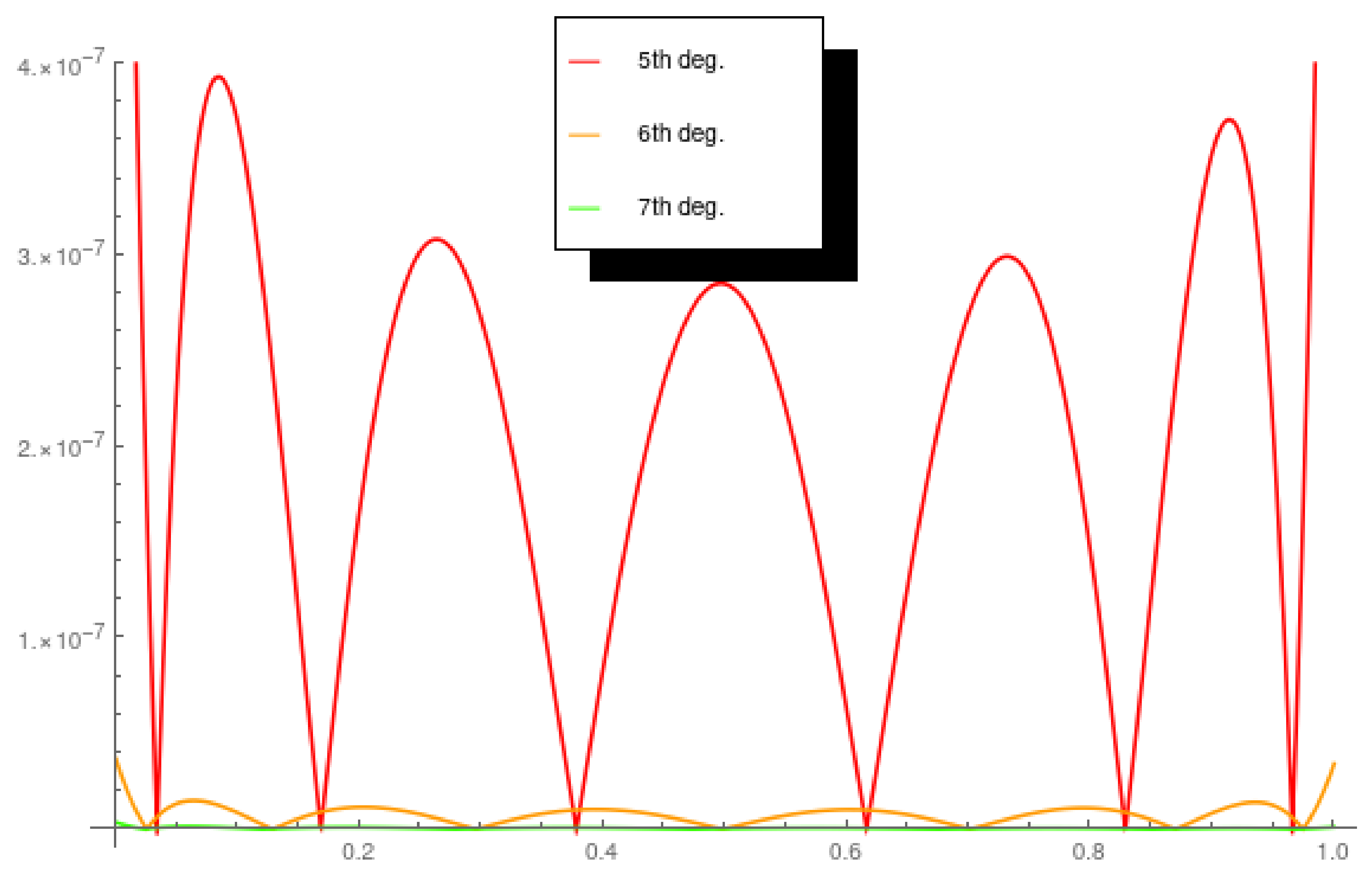
Figure 2. The absolute errors of the 5th, 6th and 7th degree PLSM approximations for problem (15).

Again, the comparison in Table 3 clearly shows the precision of our method and, together with Figure 2, at the same time illustrates its quick convergence.

3.5. Application 5: Volterra–Fredholm Integro-Differential Equation

The next example is the Volterra–Fredholm integro-differential equation together with the corresponding condition ([22]):

$$\begin{array}{c}{u}^{\prime }\left(x\right)-5\times exp(x-1)+2\times exp\left(x\right)+x^2\times sin\left(2x\right)-2x+2\times sin\left(x\right)-2\times sin\left(2x\right)\\ +2x\times cos\left(2x\right)-\underset{0}{\overset{1}{\int }}exp(x-s)\times u\left(s\right)ds-\underset{0}{\overset{x}{\int }}cos(x+s)\times u\left(s\right)ds=0,\\ x\left(0\right)=0.\end{array}$$

(16)

While the errors of the approximation computed in ([22]) are of the order of ${10}^{-3}$, by using PLSM, we can find the exact solution of (16), $u_e=x^2$.

3.6. Application 6: Fourth Order Nonlinear Volterra–Fredholm Integro-Differential Equation

The next example is the nonlinear Volterra–Fredholm integro-differential equation together with the corresponding conditions ([24]):

$$\begin{array}{c}{x}^4\times u^{\left(4\right)}\left(x\right)-u^{″}\left(x\right)+u^{\prime }\left(x\right)+{\displaystyle \frac{x^6}{30}}+{\displaystyle \frac{x^4}{6}}+{\displaystyle \frac{x^2}{2}}-{\displaystyle \frac{14x}{3}}+{\displaystyle \frac{1}{2}}\\ -\underset{0}{\overset{x}{\int }}(x-s)\times u^2\left(s\right)ds+2\times \underset{0}{\overset{1}{\int }}(x+s)\times u\left(s\right)ds=0,\\ x\left(0\right)=1,x^{\prime }\left(0\right)=0,x^{″}\left(0\right)=2,x^{‴}\left(0\right)=0.\end{array}$$

(17)

Using PLSM, we can find again the exact solution, $u_e=x^2+1$.

3.7. Application 7: Eighth Order Volterra–Fredholm Integro-Differential Equation

The last example is the Volterra–Fredholm integro-differential equation together with the corresponding conditions ([18,19]):

$$\begin{array}{c}{u}^{\left(8\right)}\left(x\right)-u\left(x\right)+8\times e^x-x^2-\underset{0}{\overset{1}{\int }}{x}^2\times u^{\prime }\left(s\right)ds=0,\\ x\left(0\right)=1,x^{\prime }\left(0\right)=0,x^{″}\left(0\right)=-1,x^{‴}\left(0\right)=-2,\\ x^{\left(4\right)}\left(0\right)=-3,x^{\left(5\right)}\left(0\right)=-4,x^{\left(6\right)}\left(0\right)=-5,x^{\left(7\right)}\left(0\right)=-6.\end{array}$$

(18)

The problem has the exact solution $u_e=(1-x)\times e^x$.

Table 4 shows the comparison between our solutions and the solutions computed in [18] by using the variational iteration method (15th degree polynomial) and in [19] by using a projection method based on generalized Bernstein polynomials (15 terms).

Table 4. Absolute errors of the approximations for problem (18).

x	[18] 15th	[19] $\mathit{n}=15$	PLSM 13th	PLSM 14th	PLSM 15th
0.2	$1.1\times {10}^{-16}$	$1.6\times {10}^{-12}$	$6.7\times {10}^{-16}$	$1.1\times {10}^{-16}$	$1.1\times {10}^{-16}$
0.4	$1.2\times {10}^{-14}$	$1.7\times {10}^{-12}$	$6.3\times {10}^{-14}$	$1.1\times {10}^{-15}$	$1.0\times {10}^{-16}$
0.6	$6.6\times {10}^{-13}$	$1.4\times {10}^{-12}$	$4.5\times {10}^{-13}$	$4.2\times {10}^{-15}$	$1.1\times {10}^{-16}$
0.8	$1.2\times {10}^{-11}$	$6.3\times {10}^{-13}$	$1.2\times {10}^{-12}$	$5.4\times {10}^{-15}$	$5.6\times {10}^{-17}$
1.0	$1.1\times {10}^{-10}$	$8.0\times {10}^{-12}$	$1.9\times {10}^{-12}$	$5.3\times {10}^{-15}$	$1.7\times {10}^{-17}$

4. Conclusions

The paper presents the polynomial least squares method as a simple and straightforward but efficient and accurate method to calculate approximate polynomial solutions for nonlinear integro-differential equations of the Fredholm and Volterra type.

The main advantages of PLSM are as follows:

• The simplicity of the method—the computations involved in PLSM are as straightforward as possible (in fact, in the case of a lower degree polynomial, the computations can be easily carried out by hand; see Application 1).
• The accuracy of the method—this is well illustrated by the applications presented since by using PLSM, we could compute approximations more precisely than the ones computed in previous papers. We remark that, even though we only included a handful of (significant) test problems, we actually tested the method on most of the usual test problems for this type of equation. In all the cases when the solution was a polynomial (which is a frequent case), we could find the exact solution, while in the cases when the solution was not polynomial, most of the time we were able to find approximations that were at least as good (if not better) than the ones computed by other methods.
• The simplicity of the approximation—since the approximations are polynomial, they also have the simplest possible form and thus, any subsequent computation involving the solution can be performed with ease. While it is true that for some approximation methods which work with polynomial approximations the convergence may be very slow, this is not the case here (see, for example, Application 2, Application 4 and Application 7, which are representative for the performance of the method).

We remark that the class of equations presented here is a very general one, including most of the usual integro-differential Fredholm and Volterra problems. However, we also wish to remark that since the method itself is not really dependent on a certain expression of the equation, it could be easily adapted to solve other different types of difficult problems.

References

- Benchohra, M.; Rezoug, N. Existence and attractivity of solutions of semilinear Volterra type integro-differential evolution equations. Surv. Math. Its Appl. 2018, 13, 215–235. [Google Scholar]
- Tunç, C.; Tunç, O. On the stability, integrability and boundedness analyses of systems of integro-differential equations with time-delay retardation. Rev. Real Acad. Cienc. Exactas Físicas Nat. Ser. A. Mat. 2021, 115. [Google Scholar] [CrossRef]
- Maleknejad, K.; Mahmoudi, Y. Taylor polynomial solution of high-order nonlinear Volterra-Fredholm integro-differential equations. Appl. Math. Comput. 2003, 145, 641–653. [Google Scholar] [CrossRef]
- Wang, K.; Wang, Q. Taylor collocation method and convergence analysis for the Volterra–Fredholm integral equations. J. Comput. Appl. Math. 2014, 260, 294–300. [Google Scholar] [CrossRef]
- Hosseini, S.M.; Shahmorad, S. Numerical piecewise approximate solution of Fredholm integro-differential equations by the Tau method. Appl. Math. Model. 2005, 29, 1005–1021. [Google Scholar] [CrossRef]
- Hosseini, S.M.; Shahmorad, S. Tau numerical solution of Fredholm integro-differential equations with arbitrary polynomial bases. Appl. Math. Model. 2003, 27, 145–154. [Google Scholar] [CrossRef]
- Ghasemi, M.; Tavassoli, M.; Babolian, E. Application of He’s homotopy perturbation method to nonlinear integro-differential equations. Appl. Math. Comput. 2007, 188, 538–548. [Google Scholar] [CrossRef]
- Yüzbaşi, Ş.; Sezer, M.; Kemanci, B. Numerical solutions of integro-differential equations and application of a population model with an improved Legendre method. Appl. Math. Model. 2013, 37, 2086–2101. [Google Scholar] [CrossRef]
- Lakestani, M.; Saray, B.N.; Dehghan, M. Numerical solution for the weakly singular Fredholm integro-differential equations using Legendre multiwavelets. J. Comput. Appl. Math. 2011, 235, 3291–3303. [Google Scholar] [CrossRef] [Green Version]
- Bhrawya, A.H.; Tohidic, E.; Soleymanic, F. A new Bernoulli matrix method for solving high-order linear and nonlinear Fredholm integro-differential equations with piecewise intervals. Appl. Math. Comput. 2012, 219, 482–497. [Google Scholar] [CrossRef]
- Sathar, M.H.A.; Rasedee, A.F.N.; Ahmedov, A.A.; Bachok, N. Numerical Solution of Nonlinear Fredholm and Volterra Integrals by Newton-Kantorovich and Haar Wavelets Methods. Symmetry 2020, 12, 2034. [Google Scholar] [CrossRef]
- Amin, R.; Shah, K.; Asif, M.; Khan, I. Efficient numerical technique for solution of delay Volterra-Fredholm integral equations using Haar wavelet. Heliyon 2020, 6, e05108. [Google Scholar] [CrossRef] [PubMed]
- Islam, S.; Aziz, I.; Al-Fhaid, A.S. An improved method based on Haar wavelets for numerical solution of nonlinear integral and integro-differential equations of first and higher orders. J. Comput. Appl. Math. 2014, 260, 449–469. [Google Scholar] [CrossRef]
- Ming, W.; Huanga, C. Collocation methods for Volterra functional integral equations with non-vanishing delays. Appl. Math. Comput. 2017, 296, 198–214. [Google Scholar] [CrossRef]
- Davaeifar, S.; Rashidinia, J. Boubaker polynomials collocation approach for solving systems of nonlinear Volterra–Fredholm integral equations. J. Taibah Univ. Sci. 2017, 11, 1182–1199. [Google Scholar] [CrossRef]
- Buranay, S.C.; Özarslan, M.A.; Falahhesar, S.S. Numerical solution of the Fredholm and Volterra integral equations by using modified Bernstein–Kantorovich operators. Mathematics 2021, 9, 1193. [Google Scholar] [CrossRef]
- Maleknej, K.; Attary, M. An efficient numerical approximation for the linear class of Fredholm integro-differential equations based on Cattani’s method. Commun. Nonlinear Sci. Numer. Simul. 2011, 16, 2672–2679. [Google Scholar] [CrossRef]
- Shang, X.; Han, D. Application of the variational iteration method for solving nth-order integro-differential equations. J. Comput. Appl. Math. 2010, 234, 1442–1447. [Google Scholar] [CrossRef] [Green Version]
- Acar, N.I.; Daşcioglu, A. A projection method for linear Fredholm–Volterra integro-differential equations. J. Taibah Univ. Sci. 2019, 13, 644–650. [Google Scholar] [CrossRef] [Green Version]
- Sabzevari, M. A review on “Numerical solution of nonlinear Volterra-Fredholm integral equations using hybrid of ...” [Alexandria Eng. J. 52 (2013) 551–555]. Alex. Eng. J. 2019, 58, 1099–1102. [Google Scholar] [CrossRef]
- Hosry, A.; Nakad, R.; Bhalekar, S. A hybrid function approach to solving a class of Fredholm and Volterra integro-differential equations. Math. Comput. Appl. 2020, 25, 30. [Google Scholar] [CrossRef]
- Rahmani, L.; Mordad, M. Numerical solution of Volterra-Fredholm integro-differential equation by Block Pulse functions and operational matrices. Gen. Math. Notes 2011, 4, 37–48. [Google Scholar]
- Maturi, D.A.; Simbawa, E.A.M. The modified decomposition method for solving volterra fredholm integro-differential equations using maple. Int. J. GEOMATE 2020, 18, 84–89. [Google Scholar] [CrossRef]
- Behiry, S.; Mohamed, S. Solving high-order nonlinear Volterra-Fredholm integro-differential equations by differential transform method. Nat. Sci. 2012, 4, 581–587. [Google Scholar] [CrossRef] [Green Version]
Publisher’s Note: MDPI stays neutral with regard to jurisdictional claims in published maps and institutional affiliations. |
© 2021 by the authors. Licensee MDPI, Basel, Switzerland. This article is an open access article distributed under the terms and conditions of the Creative Commons Attribution (CC BY) license (https://creativecommons.org/licenses/by/4.0/).